VALUATION OF AMERICAN INTEREST RATE OPTIONS BY THE LEAST-SQUARES MONTE CARLO METHOD
Claudia Dourado Cescato
1*and Eduardo Fac´o Lemgruber
2Received June 17, 2009 / Accepted March 31, 2011
ABSTRACT.The purpose of this study is to verify the efficiency and the applicability of the Least-Squares Monte Carlo method for pricing American interest rate options. Results suggest that this technique is a promising alternative to evaluate American-style interest rate options. It provides accurate option price estimates which are very close to results provided by a binomial model. Besides, actual implementation can be easily adapted to accept different interest rate models.
Keywords: American options, interest rate, Monte Carlo Simulation.
1 INTRODUCTION
In spite of the increasing variety of financial instruments with American-style embedded options there isn’t a closed-form valuation formula for pricing these securities. In general, the valuation of these types of derivatives requires not only the choice of a stochastic process to represent the interest rate evolution, but also the description of the fixed income instrument price behavior. This article suggests the use of the Least-Squares Monte Carlo method, proposed by Longstaff & Schwartz (2001) as a solution for the valuation of American-style interest rate options. The Least-Squares Monte Carlo method is a well-suited technique for pricing fixed income American options, because it accepts many stochastic processes for the interest rate and supports several risk factors, such as the credit risk and the liquidity risk.
A technique widely applied in the valuation of American interest rate options is the binomial model. Rendleman & Bartter (1980) use this technique for pricing European and American bond options. Their model supposes that the short rate follows the geometric Brownian motion dynamics. Nelson & Ramaswamy (1990) present the binomial model as a practical and effective tool for pricing interest rate options. Through the development of a general technique of building recombining binomial trees, the authors suggest that the method can be applied to all dynamics
*Corresponding author
used for modeling the interest rate behavior. Black, Derman & Toy (1990) apply the binomial model to evaluate options embedded in American Treasury Bonds, considering that the short rate follows a lognormal distribution. Boyle, Evnine & Gibbs (1989) present a multidimensional extension of the binomial model that can be used for pricing European and American options subject to several risk factors. However, it is necessary to stand out that the binomial model is hardly used for pricing interest rate options subject to two or more risk factors, since the number of nodes in the tree grows exponentially with the number of risk factors.
The use of Monte Carlo simulation for pricing American-style options still remains a challenge in finance. Bossaerts (1989) was one of the first authors to suggest that the method could be applied to value American options. Bossaerts’ approach, known as parametric approach, con-sists of modeling the exercise region of an American option by a parametric function and then finding the highest value of the option in this area. A few years later, Broadie & Glasserman (1997) presented another simulation approach for pricing American-style options: the random tree approach. Both approaches, however, have strong limitations. The parametric approach can’t always be applied to price securities with several risk factors, while the random tree approach is not appropriate for pricing American-style options with six or more exercise dates. In 2001, Longstaff & Schwartz developed a promising technique to evaluate American-style options by simulation that supports any number of risk factors and exercise dates: the Least-Squares Monte Carlo method. The purpose of this method is to provide the optimal exercise strategy and to value the American type option, through an optimization algorithm based on least-squares regression. The authors applied this technique to evaluate American put options, American-Asian options, swaptions and cancelable index amortizing swaps.
2 METHODOLOGY
The Least-Squares Monte Carlo (LSM) method is a technique for pricing American options that combines Monte Carlo Simulation with an optimization algorithm based on regression. Accord-ing to Longstaff & Schwartz (2001), it is a flexible approach that supports several risk factors and accepts any type of dynamics for those factors. Simplicity, easiness to apply and computational efficiency are other advantages of their technique. On the other hand, as every simulation method it can produce biased estimates for option prices when the number of trials is small.
The purpose of LSM method is to provide the optimal exercise strategy of the American option and, consequently, its price. The intuition behind the method is that the holder of an American option decides to exercise it by comparing the payoff from immediate exercise with the expected payoff from continuation, that is, the expected option value if it’s not exercised. In other words, the estimation of the conditional expectation function for each exercise date defines the optimal exercise strategy of the option. The expected payoff from continuation can be estimated by a least-squares regression, in which the independent variables are basic functions of option state variables and the dependent variable is the discounted payoff from keeping the option alive and exercising it at future dates.
The use of LSM algorithm for pricing American-style interest rate options requires the choice of the dynamics that represents the option state variables behavior and the description of option un-derlying asset dynamic under the risk-neutral measures. In the American put valuation example presented by Longstaff & Schwartz (2001), such definitions are made at the same time, since the option state variable and the option underlying asset are the same variable: the stock price. In the particular case of interest rate options evaluated here, the state variable is the short rate and the underlying asset is the zero-coupon bond, whose stochastic process under the risk-neutral measure is:
Bt(T)=F V.EtQ
exp − T Z t
r(s).ds
(1)
where:Bt(T)is the price, at timet, of a zero-coupon bond with face valueF V, maturing at time T,ris the short rate andQis the risk-neutral measure.
One of the critical issues of applying the algorithm for pricing the interest rate options consid-ered here is to correctly describe the stochastic process for the bond price, through the analytic resolution of Equation 1. In other words, the success of the algorithm depends on the prop-erly generation of paths for the bond, starting from the simulation of the short rate paths. The formulae applied to generate these paths are presented in Appendixes I and II.
2.1 A Simple Example of LSM Algorithm
the data used in the illustration. The option can be exercised at any time prior or equal to its maturity date, except at time Zero.
Exhibit 1– Example of Valuation of an American Interest Rate Put by The LSM Method.
FV Face Value of The Bond $ 100
T2 Time to Maturity of The Bond 2 years (504 working days) T Time to Maturity of The American Put 1 year (252 working days) K Strike Price of The American Put $ 81
n2 Simulation Number of Periods until The Bond Maturity 8* n Simulation Number of Periods until Put Maturity 4 N Number of Simulated Paths for The Short Rate 8
r0 Annual Short Rate at Time Zero (continuous compounding) 15% per annum
1t Time Interval (year’s fraction) 0.25(=T2/n2)
* Each period is equal to a quarter of the year.
The first step of the algorithm consists in generating paths for the short rate using the discreet version of Vasicek dynamics’ stochastic differential equation, i.e., Appendix I, Equation (3), from Time Zero until the expiration time of the option. Exhibit 2 shows the simulated values for the short rate in each one of the eight paths.
Exhibit 2– Simulated Values for The Short Rate.
Path Time 0 Time 1 Time 2 Time 3 Time 4
(t=0) (t=0.25) (t=0.5) (t=0.75) (t=1)
1 0.1500 0.1798 0.1760 0.2951 0.4173 2 0.1500 0.1361 0.1842 0.1952 0.1713 3 0.1500 0.2453 0.2790 0.2885 0.3205 4 0.1500 0.2427 0.3260 0.1960 0.1662 5 0.1500 0.1385 0.1460 0.0818 0.0603 6 0.1500 0.0356 0.1354 0.2038 0.1760 7 0.1500 0.1408 0.1257 0.1459 0.1607 8 0.1500 0.1000 0.1662 0.1796 0.2814
Exhibit 3– Bond Prices.
Path Time 0 Time 1 Time 2 Time 3 Time 4
(t=0) (t=0.25) (t=0.5) (t=0.75) (t=1)
1 75.4940 75.8527 * 78.8476 * 74.4078 * 71.8814 * 2 75.4940 79.0407 * 78.2865 * 80.5227 * 85.1444 3 75.4940 71.3172 * 72.0613 * 74.7971 * 76.8335 * 4 75.4940 71.4915 * 69.1654 * 80.4688 * 85.4395 5 75.4940 78.8621 * 80.9409 * 88.0709 91.8996 6 75.4940 86.8806 81.6938 79.9789 * 84.8681 7 75.4940 78.6918 * 82.3856 83.7203 85.7658 8 75.4940 81.7721 79.5232 * 81.5187 78.9295 *
For each simulated path, starting from Time 3, the time immediately before the expiration time until Time 1, the algorithm chooses between exercising the option at that time or waiting to exercise the option in the future. Therefore, at each time, from Time 3 to Time 1, the algorithm compares the payoff from immediate exercise with the expected option payoff from continuation. If the payoff from immediate exercise is greater than the payoff from continuation, the option is exercised. Otherwise, the option stays alive. The payoff from continuation at each time is estimated by a least-squares regression. In this example, a multiple regression is used, where the independent variables are the short rate(X)at a given time and its square(X2), while the dependent variable(Y)is the discounted value of cash flows due to exercise of the option at the following periods.
The regression estimated function is called Conditional Expectation Function. Only the paths where the option can be exercised are used in the estimation procedure. At Time 3, the option can be exercised in Paths 1, 2, 3, 4 and 6. Exhibit 4 shows the values of the dependent variable
(Y)and the independent variables (X andX2)used for estimating the Conditional Expectation Function at Time 3. The value of the dependent variable (Y)at Time 3 is the payoff from exercising the option at Time 4 discounted back to Time 3 by the short rate at Time 3. For example, in the case of Path 1, in which the option value at the expiration time is $9.1186, the value ofY is $9.1186x e−(0.2951x0.25) =$8.4700. The Conditional Expectation Function estimated at Time 3 is presented at the bottom of Exhibit 4.
Exhibit 4– Time 3 Data used for Estimating the Conditional Expec-tation Function and the Estimated Conditional ExpecExpec-tation Function.
Path Y∗ Short rate(X) Short rate2(X2)
1 8.4700 0.2951 0.0871
2 0.0000 0.1952 0.0381
3 3.8766 0.2885 0.0832
4 0.0000 0.1960 0.0384
6 0.0000 0.2038 0.0415
* Present value of cash flows due to exercise of the option at Time 4 discounted back to Time 3 by the short rate at Time 3.
The Estimated Conditional Expectation Function is used to calculate the expected payoff from continuation for the paths where the option can be exercised (1, 2, 3, 4 and 6). Exhibit 5 presents the payoffs from immediate exercise, the expected payoffs from continuation and the exercise decisions made at Time 3. The payoff from immediate exercise at Time 3 is equal to the difference between the option strike price and the bond price at Time 3. For example, in Path 1, the payoff from immediate exercise is ($81−$74.4078)= $6.5922. The expected payoff from continuation of the option at Time 3 is($147.39−$1295.11×0.2951+$2780.38×
(0.2951)2)=$7.3424. Since this value is greater than the payoff from immediate exercise, the resulting decision is to wait to exercise the option in the future. Exhibit 5 summarizes Time 3 exercise results.
Exhibit 5– Time 3 Optimal Early Exercise Decision.
Path Immediate Expected payoff Decision exercise from continuation
1 6.5922 7.3424 <===wait 2 0.4773 0.5320 <===wait 3 6.2029 5.1783 <=== exercise 4 0.5312 0.3563 <=== exercise 6 1.0211 –1.0624 <=== exercise
Exhibit 6 presents the resulting option cash flows for the exercise procedures obtained above. Path 1 cash flow at Time 3 is zero because the option is not exercised at this time, and the cash flow at Time 4 (expiration time) is $9.1186, the option value at expiration time. In this case, the waiting decision is followed by an exercise decision. For Path 2, the waiting decision at Time 3 is not followed by an exercise decision at Time 4, because the bond price at expiration ($85.1444) is greater than the option strike price ($81).
Exhibit 6– Time 3 Option Partial Cash Flows.
Path Time 3 Time 4
(t=0.75) (t=1)
1 – 9.1186
2 – –
3 6.2029 –
4 0.5312 –
5 – –
6 1.0211 –
7 – –
8 – 2.0705
Exhibit 7– Time 2 Data Used for Estimating the Conditional Expectation Function and The Estimated Conditional Expectation Function.
Path Y∗ Short rate(X) Short rate2(X2)
1 8.1055 0.1760 0.0310
2 0.0000 0.1842 0.0339
3 5.7850 0.2790 0.0778
4 0.4896 0.3260 0.1063
5 0.0000 0.1460 0.0213
8 1.8990 0.1662 0.0276
* Present value of cash flows due to exercise of the option at Times 3 or 4 discounted back to Time 2.
E[Y|X] = −34.88+345.67X−724.83X2
Exhibit 8 shows the payoffs from immediate exercise, the expected payoffs from continuation and the exercise decisions for Time 2. According to these decisions, the algorithm builds the partial cash flows of all paths starting from Time 2, presented in Exhibit 9. Paths 1, 6 and 8 cash flows are maintained, while Paths 3 and 4 cash flows are modified, due to the decisions made by the algorithm at Time 2.
Exhibit 8– Time 2 Optimal Early Exercise Decision.
Path Immediate Expected payoff Decision exercise from continuation
1 2.1524 3.4996 <===wait 2 2.7135 4.1915 <===wait 3 8.9387 5.1353 <=== exercise 4 11.8346 0.7758 <=== exercise 5 0.0591 0.1309 <===wait 8 1.4768 2.5460 <===wait
Exhibit 9– Time 2 Option Partial Cash Flows.
Path Time 2 Time 3 Time 4
(t=0.5) (t=0.75) (t=1)
1 – – 9.1186
2 – – –
3 8.9387 – –
4 11.8346 – –
5 – – –
6 – 1.0211 –
7 – – –
At Time 1, according to Exhibit 3, the option can be exercised in Paths 1, 2, 3, 4, 5 and 7. Exhibit 10 shows the values of the dependent variable(Y)and the independent variables (X and X2) used for estimating the Conditional Expectation Function of the option at Time 1 and its equation. Exhibit 11 presents the payoffs from immediate exercise, the expected payoffs from continuation and the decisions about the early exercise of the option at Time 1.
Exhibit 10– Time 1 Data Used for Estimating the Conditional Expectation Function and The Estimated Conditional Expectation Function.
Path Y∗ Short rate(X) Short rate2(X2)
1 7.7492 0.1798 0.0323
2 0.0000 0.1361 0.0185
3 8.4071 0.2453 0.0601
4 11.1380 0.2427 0.0589
5 0.0000 0.1385 0.0192
7 0.0000 0.1408 0.0198
* Present value of cash flows due to exercise of the option at Times 2, 3 or 4 discounted back to Time 1.
E[Y|X] = −62.91+660.27X−1485.75X2
Exhibit 11– Time 1 Optimal Early Exercise Decision.
Path Immediate Expected payoff Decision exercise from continuation
1 5.1473 7.7721 <===wait 2 1.9593 -0.5774 <=== exercise 3 9.6828 9.6555 <=== exercise 4 9.5085 9.8231 <===wait 5 2.1379 0.0288 <=== exercise 7 2.3082 0.5923 <=== exercise
Finally, the algorithm provides the Option Cash Flow Matrix from Time 1 until the expiration time, for all the eight simulated paths. The American put estimated value provided by the algo-rithm is $4.5518, obtained by averaging the discounting cash flows presented in Exhibit 12.
2.2 The Script for Pricing American-Style Interest Rate Options by The LSM Method The script used for pricing American-style interest rate options is summarized in Exhibit 13. It’s a synthesis of Section 2.1 Example, constructed to facilitate the implementation of LSM method.
2.3 Data and Conventions
diffu-Exhibit 12– Option Cash Flow Matrix.
Path Time 1 Time 2 Time 3 Time 4
(t=0.25) (t=0.5) (t=0.75) (t=1)
1 – – – 9.1186
2 1.9593 – – –
3 9.6828 – – –
4 – 11.8346 – –
5 2.1379 – – –
6 – – 1.0211 –
7 2.3082 – – –
8 – – – 2.0705
Exhibit 13– Script for Pricing American-Style Interest Rate Options by The LSM Method.
1. Generate 1,000 (or 10,000) paths for the short rate from Time Zero until the expiration time of the option, using the formulas presented in Appendix I.
2. Generate 1,000 (or 10,000) paths for the fixed income bond price from Time Zero until the expiration time of the option, using the formulas presented in Appendix II.
3. Calculate the option payoff at the expiration time for each simulated path.
4. From the time immediately before the expiration time until Time 1:
– Estimate the Conditional Expectation Function by least-squares regression.
– Calculate the option payoff from immediate exercise for the paths where the option can be exercised.
– Calculate the expected option payoff from continuation for the paths where the option can be exercised.
– Decide to exercise the option if the expected payoff from continuation is smaller than the payoff from immediate exercise.
– Build the partial cash flows of all paths, starting from current time until the expiration time of the option.
5. Calculate the option value estimate corresponding to one simulation run by averaging the discounting cash flows of all paths.
sion coefficient, in order to present a more similar behavior. Besides, the drift of Rendleman and Bartter model was eliminated, assuring that the short rate exhibits the same mean reversion behavior found in Vasicek and CIR models.
Exhibit 14– Interest Rate Dynamics. Rendleman and Bartter Model:dr=μr dt+σr d z
σ Diffusion coefficient 10% per annum
20% per annum
μ Drift coefficient 0.5% per annum(=σ
2/2)∗
2% per annum(=σ2/2)∗ Vasicek Model:dr=a(b−r)dt+σd z
b Annual long-term interest rate (continuous compounding) 15% per annum a Reversion speed of short rate to long-term interest rate 80%
σ Diffusion coefficient 10% per annum
20% per annum CIR Model:dr=a(b−r)dt+σ√r d z
b Annual long-term interest rate (continuous compounding) 15% per annum a Reversion speed of short rate to long-term interest rate 80%
σ Diffusion coefficient 10% per annum
20% per annum
Note:ris the short rate,dtis the infinitesimal time interval andd zis the random component, extracted from a Normal distribution with mean zero and variancedt(Wiener process).
*The choice of these values for the drift coefficient eliminates the process trend.
Exhibit 15– Data Used in Simulations and Binomial Trees.
F V Face value of the bond $100
T2 Times to maturity of the bond 42 working days (0.17 years) 84 working days (0.33 years)
T Times to maturity of the options 21 working days (0.08 years) 42 working days (0.17 years)
K Strike prices of the calls ($) 94.5, 95, 95.5 and 96 Strike prices of the puts ($) 99.5, 100, 100.5 and 101 r0 Annual short rate at Time Zero (continuous compounding) 15% per annum
ns Number of steps (dimensions) 168
1t Time interval (year’s fraction) (T2/252)/ns
N Number of trials of each simulation run (paths) 10,000 (Vasicek and CIR) 1,000 (Rendleman and Bartter)
nr Number of simulation runs 20
and CIR trees are built based on the methodology developed by Nelson & Ramaswamy (1990). Regarding the implementation of LSM method, the independent variables used for estimating the Conditional Expectation Function are the short rate(X), its square(X2)and its cube(X3), as suggested by Longstaff & Schwartz. Besides, in order to minimize the standard error of the estimates provided by the algorithm, simulations are executed with a variance reduction tech-nique and with, at least, 1,000 paths. The variance reduction techtech-nique used in this study is the Descriptive Sampling (DS), suggested by Saliby (1990) as a sampling procedure that is better than a Simple Random Sampling (SRS) regarding statistical accuracy and simulation processing time. Saliby, Gouvˆea & Marins (2007) use Descriptive Sampling on a Monte Carlo simulation to price European stock options and conclude that the estimates provided by this technique are more accurate than the estimates provided by SRS.
2.4 Rendleman & Bartter, Vasicek and CIR Dynamic Preliminary Tests
In order to test the implementation of the discreet versions of interest rate dynamics as well as the implementation of bond stochastic processes we performed several preliminary tests focusing on the valuation of European interest rate options by simulation. Simulations using the Rendleman and Bartter dynamics are executed with only 1,000 paths for short rates and bond prices, because bond price calculations require a high computational time.
Results are shown in Tables 1 and 2. The observed biases are very close to zero, indicating that the European interest rate option estimates provided by Monte Carlo Simulation converge to the available analytic solutions and to the results provided by the binomial model. Besides, standard errors and the root mean squared errors (RMSE) are very small indicating that estimates are accurate. For all dynamics, an increase of the diffusion coefficient from 10% to 20% does not affect the estimate bias. Indeed, test repetition with other values for the diffusion coefficient shows that the estimate bias is not affected by the variation of this parameter. Test results also reveal that varying the strike price of the in-the-money or at-the-money options does not impact the standard error of the estimates. A complete analysis of the results for the European interest rate options is presented by Cescato (2008).
3 RESULTS
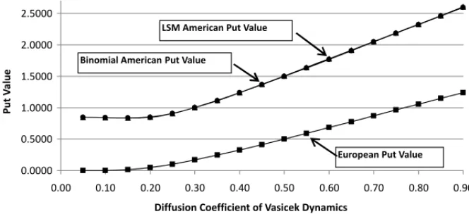
Figure 1– Values of an American Put Embedded in a Zero-Coupon Fixed Income Bond for Different Diffusion Coefficients of Vasicek Dynamics. The American put value curve provided by the binomial model and the American put value curve provided by the LSM method are overlapped,i.e., the convergence of Least-Squares Monte Carlo estimates to results provided by the binomial model does not depend on the diffusion coefficient value of Vasicek dynamics. The estimates are generated through the simulation of 10,000 paths (with 168 steps) for the short rate, using Descriptive Sampling. The bond’s face value is $100 and it expires in 4 months (84 working days). The strike price of the American put is $96, the current short rate is 15% per annum, the long-term interest rate is 15% per annum and the reversion speed of short rate to long-term interest rate is 80%.
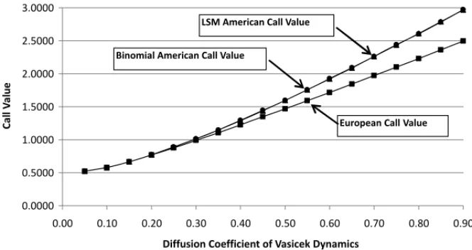
Results presented in Tables 1 and 3 reveal that there is no value to the right of the early exercise of an American interest rate call since their values are very close to the European interest rate calls with the same strike price. According to the literature, this occurs because the payoff from the early exercise of an American call is always smaller than the derivative value. Indeed, this conclusion applies to any dynamics which does not accept negative interest rates, like Rendleman and Bartter and CIR dynamics, but it does not apply to the Vasicek dynamics. Figure 3 reveals that, in the specific case of Vasicek dynamics, as the diffusion coefficient reaches higher levels, the values of the American calls depart from the values of the European calls, i.e., it becomes better to exercise the American call before the expiration time. Regarding the American puts, Tables 2 and 4 reveal that their values are greater than the values of the corresponding European puts. For example, the values of the American puts with strike price equal to $100 are about twice the values of the European puts with the same strike price. The difference between the value of an American put and the value of a European put with the same strike price is explained by the value due to the right of the early exercise. Unlike the European put, which can only be exercised at the expiration time, the American put can be exercised at any time before or equal to the expiration time. As the early exercise of an American put can provide a cash flow greater than the value paid for the option, the value of an American put will always be greater than the value of a European put with the same strike price.
Figure 3– Values of an American Call Embedded in a Zero-Coupon Fixed Income Bond for Different Diffusion Coefficients of Vasicek Dynamics. As the diffusion coefficient reaches higher levels, it becomes better to exercise the American call before the expiration. The estimates are generated through the simula-tion of 10,000 paths (with 168 steps) for the short rate, using Descriptive Sampling. The bond’s face value is $100 and it expires in 4 months (84 working days). The strike price of the American call is $97, the current short rate is 15% per annum, the long-term interest rate is 15% per annum and the reversion speed of short rate to long-term interest rate is 80%.
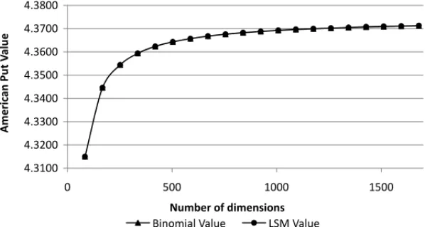
is not very small. This bias can be eliminated increasing the number of dimensions used in the simulations, as illustrated in Figure 4.
Figure 4– Values of an American Put Embedded in a Zero-Coupon Fixed Income Bond for Different Numbers of Simulation Steps (Dimensions). Short rate follows the CIR dynamics. The Least-Squares Monte Carlo estimates converge to results provided by the binomial model, regardless of the number of dimensions used. The estimates are generated through the simulation of 1,000 paths for the short rate, using Descriptive Sampling. The bond’s face value is $100 and it expires in 4 months (84 working days). The strike price of the American put is $99.5, the current short rate is 15% per annum, the long-term interest rate is 15% per annum, the reversion speed of short rate to long-term interest rate is 80% and the diffusion coefficient of CIR dynamics is 10% per annum.
4 CONCLUSION
The purpose of this study is to verify the efficiency and the applicability of the Least-Squares Monte Carlo (LSM) method for pricing American interest rate options. Rendleman and Bartter, Vasicek and CIR models, which are very popular, are used to model the interest rate behavior. Results from several simulations show that the LSM method is an effective tool for pricing Amer-ican interest rate options. It provides accurate estimates which are very close to results provided by the binomial model.
Concerning the possibility of early exercise, results show that the American interest rate put values are greater than the European put values with the same strike price in all simulations. Regarding the American calls, results suggest that the payoff from early exercise is tied to the dynamics used to model the interest rate behavior. For the dynamics that accepts negative interest rates, the case of Vasicek model, it can be profitable to exercise the American call before the expiration time. Otherwise, if the chosen dynamics does not accept negative interest rates, the case of Rendleman and Bartter and CIR models, it will never be better to exercise the American call before maturity.
binomial model. Unlike the binomial model, the LSM method, once implemented, can be easily adapted to accept any new interest rate dynamics. The flexibility of LSM method makes itself an important technique for pricing options and derivatives subject to market risk, since there is no consensus among financial agents about which dynamics must be used to model the interest rate behavior.
REFERENCES
[1] BLACKF, DERMANE & TOYW. 1990. A One-Factor Model of Interest Rates and Its Application to Treasury Bond Options.Financial Analysts Journal,46: 33–39.
[2] BOYLEP, EVNINEJ & GIBBSS. 1989. Numerical Evaluation of Multivariate Contingent Claims. The Review of Financial Studies,2: 241–250.
[3] BOSSAERTSP. 1989. Simulation Estimators of Optimal Early Exercise. Working Paper. Carnegie-Mellon University.
[4] BROADIEM & GLASSERMANP. 1997. Pricing American-Style Securities Using Simulation.Journal of Economic Dynamics and Control,21: 1323–1352.
[5] CESCATO C. 2008. Avaliac¸˜ao de Opc¸˜oes Americanas de Taxa de Juro: O M´etodo dos M´ınimos Quadrados de Monte Carlo. Dissertac¸˜ao de Mestrado, Instituto Coppead de Administrac¸˜ao, UFRJ, Rio de Janeiro.
[6] COX JC, INGERSOLL JE & ROSS SA. 1985. A Theory of the Term Structure of Interest Rates. Econometrica,53: 385–407.
[7] LONGSTAFFF & SCHWARTZE. 2001. Valuing American Options by Simulation: A Simple Least-Squares Approach.The Review of Financial Studies,14: 113–147.
[8] NELSOND & RAMASWAMYK. 1990. Simple Binomial Processes as Diffusion Approximations in Financial Models.The Review of Financial Studies,3: 393–430.
[9] RENDLEMANR & BARTTERB. 1980. The Pricing of Options on Debt Securities.Journal of Finan-cial and Quantitative Analysis,15: 11–24.
[10] SALIBYE. 1990. Descriptive Sampling: A Better Approach to Monte Carlo Simulation.Journal of The Operational Research Society,41: 1133–1142.
[11] SALIBY E, GOUVEAˆ S & MARINSJ. 2007. Amostragem Descritiva no Aprec¸amento de Opc¸ ˜oes Europ´eias Atrav´es de Simulac¸˜ao de Monte Carlo: O Efeito da Dimensionalidade e da Probabilidade de Exerc´ıcio no Ganho de Precis˜ao.Pesquisa Operacional,27: 1–13.
APPENDIX I – FORMULAE USED TO GENERATE SHORT RATE PATHS Rendleman and Bartter Model
ri = ri−1e
h
(μ−σ2/2)∗1t+σ∗√1t∗Zi i
(2)
where:
ri is the short rate value at Step (Period)i,
ri−1 is the short rate value at Step (Period)i−1,
1t is the time interval (year’s fraction),
μ is the drift coefficient of the dynamics,
σ is the diffusion coefficient of the dynamics and
Zi is the Standard Normal random variable of Step (Period)i. Vasicek Model
ri = (1−a.1t).ri−1+a.b.1t+ σ.
√
1t.Zi (3) where:
ri is the short rate value at Step (Period)i,
ri−1 is the short rate value at Step (Period)i−1,
1t is the time interval (year’s fraction), b is the long-term interest rate,
a is the reversion speed of short rate to long-term interest rate,
σis the diffusion coefficient of the dynamics and
Zi is the Standard Normal random variable of Step (Period)i. CIR Model
ri = (1−a.1t).ri−1+a.b.1t+ σ.√ri−1.
√
1t.Zi (4) where:
ri is the short rate value at Step (Period)i,
ri−1 is the short rate value at Step (Period)i−1,
1t is the time interval (year’s fraction), b is the long-term interest rate,
a is the reversion speed of short rate to long-term interest rate,
σ is the diffusion coefficient of the dynamics and
APPENDIX II – FORMULAE USED TO GENERATE FIXED INCOME BOND PATHS Rendleman and Bartter Model
P(t,T)=F V.N1.
N P j=1
exp −
(T/1t)−1 P i=t/1t
rj(i).1t !∗
(5)
where:
P(t,T) is the price, at timet(or Periodt/1t), of a zero-coupon bond with face valueF Vmaturing at timeT,
rj(i) is the short rate value at Periodiin path j,
1t is the time interval (year’s fraction) and
N is the number of simulated paths, set at 200, due to limitations of computational resources used in this study.
*Due to the absence, in literature, of a closed-form formula for calculating the fixed income bond price, the bond price at timetis estimated through the generation of 200 paths for the short rate, starting from timet(until timeT), for each simulated short rate path.
Vasicek Model
P(t,T)=F V.A(t,T).e−B(t,T).r(t) (6)
B(t,T)= 1−e−aa.(T−t) (7)
A(t,T)=exp
(B(t,T)−T+t)(a2.b−σ2/2)
a2 −
σ2.B(t,T)2
4.a
(8)
where:
P(t,T) is the price, at timet(or Periodt/1t), of a zero-coupon bond with face valueF Vmaturing at timeT,
r(t) is the short rate value at timet,
a is the reversion speed of short rate to long-term interest rate, b is the long-term interest rate and
σ is the diffusion coefficient of the dynamics. CIR Model
P(t,T)=F V.A(t,T).e−B(t,T).r(t) (9)
h=pa2+2.σ2 (10)
B(t,T)= 2h+(2a.(+ehh.().(Te−ht).(−1T−)t)−1) (11)
A(t,T)= h
2.h.e(a+h).(T−t)/2 2h+(a+h).(eh.(T−t)−1)
i2ab/σ2
(12)
where:
P(t,T) is the price, at timet(or Periodt/1t), of a zero-coupon bond with face valueF Vmaturing at timeT,
r(t) is the short rate value at timet,
a is the reversion speed of short rate to long-term interest rate, b is the long-term interest rate and