RAPID-TRANSIT EFFICIENCY ANALYSIS WITH THE ASSURANCE-REGION DEA METHOD
Antonio G.N. Novaes
Departamento de Engenharia Industrial Universidade Federal de Santa Catarina Florianópolis – SC
Recebido em 04/2001, aceito em 10/2001 após 1 revisão
Abstract
Rapid-transit services are a relevant part of the transportation network in most cities of the world. An important aspect of transport policy is the supply of public urban transportation. In particular, it is of interest to determine whether rapid-transit operators are working in a technically and scale-efficient way. Production analysis of transit services has been characterized by the econometric study of average practice technologies. A more recent method to study such production frontiers is Data Envelopment Analysis (DEA). It is a non-parametric method, but its application to rapid-transit, where the relations among technological variables are more strict, requires a previous structural analysis of the intervening inputs and outputs. DEA is employed in this paper to investigate the efficiency and returns to scale of 21 rapid-transit properties of the world. DEA was also used for the benchmarking of non-efficient rapid-transit properties, with special emphasis to the São Paulo’s subway system.
Keywords: rapid-transit efficiency, DEA, benchmarking.
Resumo
Os sistemas de metrô são parte relevante do transporte em muitas cidades do globo. Um aspecto importante da política de transportes é a oferta. Nesse contexto, é de interesse verificar se os operadores estão trabalhando de maneira eficiente, em termos técnicos, e no que diz respeito a ganhos de escala. A análise do processo de produção de metrôs tem sido realizada através de estudos econométricos baseados em práticas tecnológicas médias. Um método mais recente para estudar fronteiras de produção é a Análise Envoltória de Dados (DEA). Trata-se de um método não-paramétrico, mas suas aplicações a metrôs, que envolvem relações mais rígidas entre as variáveis tecnológicas, requerem uma análise prévia dos inputs e dos outputs. DEA é utilizada no artigo para analisar a eficiência e ganhos de escala de 21 metrôs. É também utilizada como instrumento auxiliar no benchmarking de metrôs não eficientes, com ênfase ao metrô de São Paulo.
1. Introduction
Rapid-transit services are a relevant part of the transportation network in most of the large cities of the world. They provide passenger services within the cities and their surroundings, with different technologies and extensions. In addition, part of the urban transportation is a major source of externalities imposed on the environment and it is deeply intertwined with locational choices. Other issues as fare structure, distributional effects among the population, regulatory aspects, private or public operation, and subsidies, have equally attracted the attention of researchers and practitioners. Within this framework, an important aspect of transportation policy is the supply of urban transportation. Although some authors, as for instance Rubin et al. (1999), have argued against the widespread use of urban rail systems in the US, the number and the size of such operating systems deserve special attention. In particular, it is of interest to determine whether urban rapid-transit operators are working in a technically and scale efficient way (Kerstens, 1996).
Production analysis of transit services has been characterized for years by the study of average practice technologies, whereby investigators fit least-square econometric functions through the middle of the data. Early Cobb-Douglas estimates of transit cost and production functions are widely encountered in the literature. More recently, recognizing that a Cobb-Douglas technology imposes restrictions on some economic effects of interest in transportation, researchers have adopted the more flexible translog approximation (Spady & Friedlaender, 1976; Viton, 1992; Berechman, 1993).
The theoretical economic concept of a production function, however, is associated with its frontier nature. This suggests that the traditionally estimated “middle of the data set”
production function is inappropriate (Oum et al., 1992). The acknowledgement of the
divergence between characteristics of average and best practice production technologies redirected attention to the development of frontier estimation technologies. One of the first empirical frontier studies of technical efficiency is due to Farrel (1957). Parametric stochastic frontier methods, based on maximum-likelihood techniques, were introduced in the literature in the late seventies and their applications have spread to virtually all fields in
economics (Aigner et al., 1977; Knox Lovell, 1995). Econometric methods have been
traditionally employed by transportation analysts to investigate the economic and productive behavior of transportation services. A relative large body of information has resulted from such studies, generating some general principles and conclusions that presently orientate practitioners and investigators in the field. The book by Berechman (1993), for example, is an effort to consolidate this knowledge in a comprehensive text.
social, technological, and environmental nature, the simple DEA formulation may not be adequate. In fact, the attributes cannot vary freely in such cases, since they are constrained by technical and operational reasons. For instance, when analyzing airline companies, with aircraft-hours, employees and fuel consumption as inputs, and carried passengers as output, the ratio between fuel consumption and aircraft-hours is limited to a certain range, depending on the airplane type and operational characteristics. Therefore, a preliminary analysis of basic technical relationships is necessary before DEA application is performed.
In this paper, we apply DEA to 21 rapid-transit properties but, in order to define the appropriate variables, a technical and statistical analysis of the data is performed beforehand. It is an advancement of previous research results reported by the author in the literature (Novaes, 1997; Novaes et al., 2000).
2. Previous Results on Rapid-Transit Production and Efficiency Analysis
In most European and Asian cities, rapid transit is regarded as a major element of city life and organization of the urban structure. Transit systems tend to rely more heavily on rail, both underground and streetcar (Wunsch, 1996). In the United States, although the use of private cars by urban commuters is quite intensive, the patronage of rapid transit services in the larger metropolitan areas is also impressive. In Latin America, on the other hand, only the major cities are provided with rapid transit systems. Their supply levels usually cover only a part of the potential travel demand. The rest of the demand for public transportation is served by buses and microbuses.
The literature on the productivity of rapid-transit transportation is scarce as compared to equivalent studies of bus firms (Viton, 1992), due perhaps to the methodological difficulties of comparing economic attributes of different transit properties located in diverse countries or regions. One exception is the United States, where a reasonable number of cities are provided with rapid-transit systems. The papers of Pozdena & Merewitz (1978) and Viton (1980) analyzed cost and productivity of rapid transit properties in the United States. Viton (1992) studied the cost-effectiveness of large multi-modal transit organizations. More recently, Wunsch (1996) investigated transit cost and productivity in Europe, including a representative number of rapid transit systems together with other urban transportation modes.
In their study on rapid transit productivity, Pozdena & Merewitz (1978) found evidence of increasing returns to scale in the long run, and of economies of density in the short run. Analyzing Pozdena and Merewitz findings, Viton (1980) presented a series of considerations, questioning their results. Predominant among them was the choice of the functional form. Pozdena and Merewitz assumed that the technology of producing rapid-transit output (vehicle miles) could be described by a generalized Cobb-Douglas technology, taking, as inputs, man-hours of labor, kilowatt-hours of electricity, and the total miles of track. Viton argued against the assumption of a Cobb-Douglas technology because the elasticities of substitution between different factors of production are important elements when analyzing transit productivity, and in the Cobb-Douglas technology these elasticities are fixed.
Philadelphia, Cleveland, Shaker Heights, and Montreal, covering the period 1960-70. A translog cost function was estimated taking total annual vehicle miles as output and three factor inputs: labor, electric power, and track. While Pozdena and Merewitz concluded that there existed economies of density throughout the industry, Viton concluded that the situation varied greatly over the sample. He found out that New York, Chicago, and the SEPTA system in Philadelphia presented short-run diseconomies of density. These results were not surprising since the companies in question serve major metropolitan areas and their systems were both old and highly congested (Viton, 1980). As for Montreal’s rapid-transit system, the results indicated slight diseconomies of density, but the t-statistic did not give support to reject the hypothesis of constant returns. The remaining systems showed economies of density, although slight.
Traditionally, production functions are estimated by first adjusting a cost function to the data. Then, making use of the Shephard’s duality lemma (Coelli et al., 1998), the corresponding production function is inferred. However, some authors impose restrictions to the use of the Shephard’s duality lemma in the analysis of the production structure of rapid-transit properties. They argue that there is no evidence that transit firms tend to minimize costs. Berechman (1993) states that since cost minimization is not, in fact, the main objective of the transit firm, the estimated cost function parameters are likely to be biased due to misspecification of the model. In this case, since the transit firm is not operating on the efficient cost curve, the estimated parameters will, therefore, reflect this inefficient behavior rather than the firm’s underlying technology.
Berechman (1993) discusses a number of possibilities for the behavior of transit managers. One of them is that the transit firm, which is usually controlled or owned by a public agency, strive to maximize the budget surplus (i.e., budget less expenditures). Since the annual budget is normally fixed or difficult to raise, this approach would lead to a cost-minimization result. The empirical evidence, presented by Berechman (1993), is that while the total budget allocated to transit firms (bus or rapid-rail transit) has increased substantially over time, neither total output nor even labor input have increased, while the unit cost of output has gone up dramatically. Hence, Berechman (1993) concludes that the hypothesis that transit managers maximize budget surplus is probably incorrect. It is more likely, according to that author, that transit managers allow costs to increase to meet the higher budgets. This also means that the transit firm is not operating on the efficient cost curve, therefore restraining the use of the cost function to analyze the underlying technology.
A third restriction to the estimation of the cost function to infer the production frontier of rapid-transit properties is the heterogeneity of the input prices prevailing in different countries or regions. As mentioned, when treating the problem through a cross-section analysis of world-wide data, as in the case focussed in this paper, the input prices can hardly be assumed constant due to different national economic policies, labor regulations, construction costs, rolling stock prices, energy costs, etc.
A fourth question is related to the multi-modal characteristic of many transit agencies. Such agencies operate an integrated fleet of busses, streetcars, and rapid transit trains. A consolidated transit organization potentially benefits from “economies of scope” (Viton, 1992). Even operating distinct modes, the transit firm may integrate the sectors dedicated to vehicle and crew scheduling, route planning, payroll, marketing, etc, allowing for cost savings. As a consequence, the separate analysis of the rail rapid transit costs, without consideration to the other modes in such cases, can lead to biased results.
Regarding this intricate body of discussions and opinions, it is opportune the introduction of new forms of analyzing the problem. Particularly, in addition to the traditional parametric approaches, Data Envelopment Analysis (DEA) has been used as a process for measuring the relative efficiency of a group of decision making units (DMUs). One of the first applications of DEA to rapid-transit analysis is due to Chu et al. (1992). Novaes (1997) applied the DEA method to a sample of rapid-transit agencies of the world, with 1996 data. Each non-efficient agency was then projected onto a point on the envelopment surface (efficient frontier) according to DEA rules. Then, taking the set of efficient rapid-transit DMUs, together with the frontier-projected DMUs, a least-square regression was performed, leading to a translog production function. Although the results were statistically satisfactory, the projected DMUs on the envelopment surface do not represent real counterparts. Therefore, the method could be criticized for being somewhat artificial. For this reason, a stochastic frontier method, based on maximum-likelihood techniques, was further used to estimate a trans-log production function to the same data (Novaes, Constantino & Souza, 2000).
3. The Variable Set
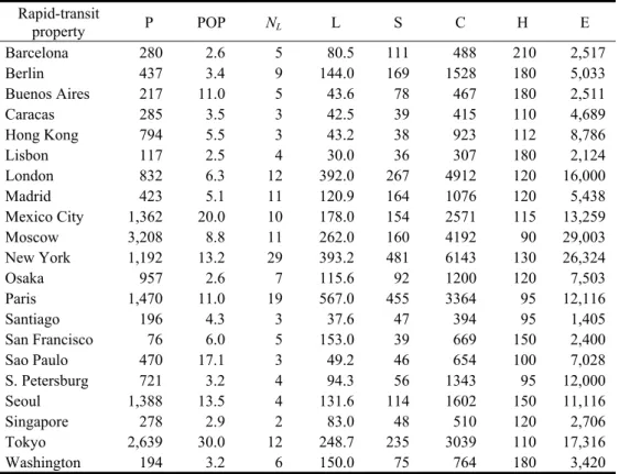
A new data set, comprising 21 rapid-transit agencies of the world, was obtained from the São Paulo’s transit agency (Cia. do Metropolitano de São Paulo, Brazil), covering the years 1999-2000. The available data are presented in Table 1. In our model, the output is represented by P, the total passengers carried per year. In order to appropriately select the independent variables of the model, a technical analysis of the production process is necessary.
3.1 Composite variable
Let us assume that a general rapid-transit property has NL lines, with extensions . On the other hand, let d be the average distance between stations, given by
NL 2
1, L , ..., L L
S L
d= , (1)
where L is the total extension of the rapid-transit lines and S is the total number of stations. Assuming an average constant speed v, the time necessary for a composition to complete a cycle on line i is given by
v L 2
T i
The number of compositions operating on line i can be expressed as a function of T and H, the peak-hour headway:
i Nt i H T k Nt i
i ≅ , (3)
where k is a constant which takes into account spare compositions parked at the depot (reserve, maintenance, etc), lost time when reversing train direction, etc. Let be the number of passenger cars allocated to line i. If u is the number of cars per train, the following relation holds
i C
i i uNt
C = (4)
Making the necessary substitutions in (4), and adding up on i, one gets
L H v u k L H v u k C C ' i i i
i = =
=
∑
2∑
(5)where C is the total number of passenger cars owned by the rapid-transit property and k’ = 2 k is a constant. From (5) one estimates u:
L H C v ' ' k
u = (6)
where
k k
2 1
''= is a constant. Passenger trip attraction in line i can be expressed as a
combination of three factors: a) the number of stations in line i; b) the train passenger capacity; and c) the peak-hour frequency of trains
, 1 H W S
Ai ≈ i× × (7)
where is the number of stations in line i. On the other hand, W is the train capacity, given by u , where w is the car capacity. Making substitutions in (7), and simplifying, one gets
i S w
. (8)
L C w v S H L H C w v S
Ai ≈ i× × 1 = i×
The total number of passengers P carried by the rapid-transit property is proportional to the sum of the Ais for all lines:
∑
= × ≈ i i L S C w v S L C w vP (9)
We admit that the effects, on the rapid-transit production, of variables v, the average train speed, and w, the average car capacity, are indirectly expressed by other inputs, such as the number of cars and the headway. This means we may approximately assume v and w to be constant in equation (9). Therefore, one important input variable to explain rapid-transit trip generation is
L S C
x1= × (10)
Table 1 – Rapid-Transit Data Rapid-transit
property P POP NL L S C H E
Barcelona 280 2.6 5 80.5 111 488 210 2,517
Berlin 437 3.4 9 144.0 169 1528 180 5,033
Buenos Aires 217 11.0 5 43.6 78 467 180 2,511
Caracas 285 3.5 3 42.5 39 415 110 4,689
Hong Kong 794 5.5 3 43.2 38 923 112 8,786
Lisbon 117 2.5 4 30.0 36 307 180 2,124
London 832 6.3 12 392.0 267 4912 120 16,000
Madrid 423 5.1 11 120.9 164 1076 120 5,438
Mexico City 1,362 20.0 10 178.0 154 2571 115 13,259
Moscow 3,208 8.8 11 262.0 160 4192 90 29,003
New York 1,192 13.2 29 393.2 481 6143 130 26,324
Osaka 957 2.6 7 115.6 92 1200 120 7,503
Paris 1,470 11.0 19 567.0 455 3364 95 12,116
Santiago 196 4.3 3 37.6 47 394 95 1,405
San Francisco 76 6.0 5 153.0 39 669 150 2,400
Sao Paulo 470 17.1 3 49.2 46 654 100 7,028
S. Petersburg 721 3.2 4 94.3 56 1343 95 12,000
Seoul 1,388 13.5 4 131.6 114 1602 150 11,116
Singapore 278 2.9 2 83.0 48 510 120 2,706
Tokyo 2,639 30.0 12 248.7 235 3039 110 17,316
Washington 194 3.2 6 150.0 75 764 180 3,420
Source: Cia. do Metropolitano de São Paulo, METRO
P – Passengers carried per year (million); POP – Served population (million); NL – Number of lines;
L – Total line extension (km); S – Number of stations; C – Number of passenger cars; H – Peak-hour headway (seconds); E – Number of employees
3.2 Peak-hour frequency (x2)
The output, total passengers carried per year, is relatively sensitive to the peak-hour frequency variation, which is given by 3,600/H, with the headway H in seconds. In fact, the renewal of passengers at the station platforms is positively influenced by train frequency, thus increasing passenger flow in the line.
3.3 Average line extension (x3)
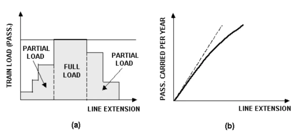
The average line extension, given by L / N L , on the other hand, has two major effects on the output. When the line extension increases, the rapid-transit spatial coverage also increases, producing a positive effect on the demand. But the line segments with partial load (edges) also tend to increase (Figure 1a), generating a curve as depicted in Figure 1b. Although the line extension L has been included into both variables x1 and x3, this fact does necessarily implies
that both variables are correlated, since the presence of L in variable x1 can be regarded
Figure 1 – Effect of subway line extension into the output
3.4 Total number of employees (x4)
The number of employees (x4) influences demand both directly and indirectly.
Train-conducting crews, being directly related to train supply, normally have a direct impact. Station personnel, on the other hand, usually have an indirect impact (ticket sales, for instance). Other activities (cleaning of the premises, maintenance, security, administration, etc.) tend to have an indirect, somewhat weaker impact.
3.5 Served population (x5)
Finally, the served population has an impact on rapid-transit production because the growth of cities is generally correlated to increasing urban concentration, mainly in the CBD areas. This concentration generates, of course, higher levels of transportation demand.
3.6 Variable preliminary analysis
A preliminary multiple regression adjustment of a logarithmic production function was
performed with the data. The correlations between the output P and the five inputs
x1,x2, … ,x5 are respectively: 0.850, 0.616, 0.326, 0.926, and 0.468. A high correlation
between x1 and the output P has confirmed the importance of that variable. Figure 2 shows
the variation of the output with x1. One can notice that, although the sample points spread
out as x1 gets larger, the correlation between the variables is apparent. The number of
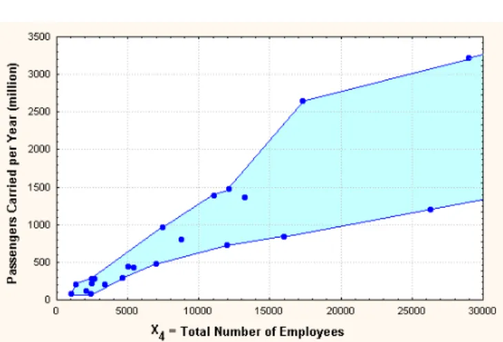
employees, on the other hand, has also shown a high correlation with the output P. In fact, it can be noticed in Figure 5 the narrower range of variation of the output with such a variable. Figure 3 shows the variation of P as a function of x2. Due to technological limitations, the
minimum headway presently attainable by conventional rapid-transit systems is 90 seconds. Therefore, the maximum frequency is 40 trains per hour. As shown in Figure 3, the points start spreading out at about x2 = 15. Consequently, we redefined the variable x2, expressing
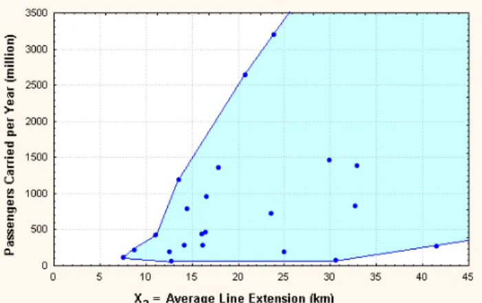
it as x'2=3600 H−15. Figure 4 shows the variation of the output P with input x3. Finally,
Figure 6 shows the variation of P with x5, the served population. It can be seen that the
Figure 2 – Output P as a function of variable x1
Figure 3 – Output P as a function of variable x2
Figure 5 – Output P as a function of variable x4
Figure 6 – Output P as a function of variable x5
4. The DEA Approach 4.1 The Basic Models
Charnes at al. (1978) extended Farrell’s (1957) approach linking the estimation of technical efficiency and production frontiers. Their initial model generalized the single output/input ratio measure of efficiency due to Farrell. The multiple output/input characterization of each DMU was transformed into a single virtual output and a single virtual input. Then, the problem was treated with a fractional linear-programming formulation. The relative technical efficiency of any DMU is calculated by forming the ratio of a weighted sum of outputs to a weighted sum of inputs. These weights are selected calculating the Pareto efficiency measure of each DMU subject to the constraint that no DMU can have a relative efficiency score greater than unity. The DMUs that attain a relative efficiency score equal to one form the frontier efficient set of DMUs (Charnes et al., 1994).
Two basic DEA models are generally used in the applications. The first, called the ratio form model, named CCR after its authors Charles, Cooper and Rhodes, allows for the evaluation of overall efficiency, identifies the efficient and non-efficient DMUs, and determines how far from the efficient frontier are the non-efficient units. The BCC model, named after its authors Banker, Charnes and Cooper (Banker et al., 1984), yields the projected efficiency point on the envelopment surface for each non-efficient DMU, together with the peer-group of efficient units associated with each non-efficient DMU (Cooper et al., 2000).
Let yk = {y1k,y2k, …,yS k} and xk = {x1k,x2k,x3k, …,xM k} be the vectors of outputs and inputs respectively for DMU k (k = 1, 2,.., n), where S and M are respectively the number of outputs and inputs considered in the analysis. Outputs and inputs are transformed into single virtual entities by weighting the values of the attributes. The single virtual output, for DMU k, is
k S S k
k
k u y u y ... u y
Y = 1 1 + 2 2 + + (11)
and the single virtual input for DMU k is
k M M k
k
k v x v x ... v x
X = 1 1 + 2 2 + + (12)
The input-oriented BCC model, with variable returns-to-scale (VRS) (Cooper et al., 2000), is
min θk (13)
subject to 0 1 ≥ −
∑
= ll l i
n
ik
k x λ x
θ , i=1,2...M (14)
k j j n y y 1 ≥
∑
= l l lλ , j=1,2...S (15)
1 1 =
∑
= n l lλ , (16)
with , and where k represents a generic DMU, θk is the efficiency score of DMU k, and n is the number of DMUs. On the other hand, the CCR model assumes constant returns to scale (CRS), and is obtained from the BCC model by suppressing constraint (16).
0 ≥
l
λ
inputs or outputs. This means that when a non-efficient DMU is projected onto a point on the envelopment surface (efficient frontier) according to DEA rules, the non-discretionary inputs and outputs remain constant, i.e. they cannot be used to upgrade a non-efficient unit.
In our application, we admitted short-term improvements only. Thus, new rapid-transit lines and new stations, as well as line extensions were considered non-discretionary variables in the DEA model. In fact, it takes a few years to plan, design and implement them. As a result, the input x1 was assumed discretionary because variable C is so. Inputs x2 and x4 are also discretionary. Since variables L and NL are non-discretionary, the input x3 is non-discretionary too. Of course, as already mentioned, the served population is a non-discretionary input.
4.2 The Assurance-Region Method
DEA assumes that the output weights u1, u2,…, uS and the input weights v1,v2, …,vM are
variable in the model, with the result that the numerous a priori assumptions and
computations involved in fixed weight choices are avoided. Thus, DEA minimizes the need for recourse to assumptions that are “outside the data” (Cooper et al., 2000). There are situations, however, in which the attributes cannot vary freely, since they are constrained by technical or operational reasons. For example, in the optimal weight vectors of DEA models for inefficient DMUs, one may see many zeros, showing that the DMU has a weakness in the corresponding items compared with other efficient DMUs. Large differences in weights from item to item may also be a concern.
The assurance-region method imposes additional constraints on the relative magnitude of the weights for special items. According to it, one may add a constraint on the ratio of weights for input i and input j, as follows (Cooper et al., 2000):
j , i i j j ,
i U
v v
L ≤ ≤ , (17)
where and U are lower and upper bounds respectively. Generally, the DEA efficiency score in the corresponding envelopment model is worsened by the additions of these constraints and a DMU previously characterized as efficient may subsequently be found to be inefficient after such constraints have been imposed (Cooper et al., 2000).
j , i
L i,j
Running the BCC model without any weight restriction, 12 of the 21 rapid-transit properties were considered efficient. Moreover, many zero weights were observed where a positive value should appear instead. Large differences in weights from item to item were also observed. Analyzing Figures 2 to 6, together with the correlations between the output P and the inputs, the following weight restrictions were introduced in the DEA model:
a) The current ways of increasing train frequency (x2) is to add more trains to the lines
(and consequently more cars), or to increase train trips per day, or both. Since the number of stations S and the total trackage L are non-discretionary inputs, the variation of input x1 tend to be close to the variation of x2. But, due to the possibility of running more train trips per day with the same number of cars, the second input can be varied with more flexibility than the first. Thus, we have assumed that the weights of x1 and x2 are limited by the following restriction:
1 2
1 v 1.3 v
b) For inputs x3, x4, and x5, the following restrictions were adopted:
1 4 v
v ≥ v1 ≥ 3 v3 v1 ≥ 5 v5 (19)
Before running the DEA model each variable was multiplied by a constant in order to impose that the largest value of each input or output is set to one hundred. This procedure, although not mandatory, is intended to avoid computing errors in the LP programming and does not affect the DEA results (scale invariance).
4.3 Efficiency analysis
We have adopted the input-oriented DEA models. This means that the non-efficient DMUs are projected on the envelopment surface (efficient frontier) by reducing the discretionary inputs, and holding the outputs constant. Both the CCR and the BCC models were applied to the data with the aid of the software EMS, version 1.3, developed by Holger Scheel (2000).
Two different sources of inefficiency can be investigated in DEA models. The first comprises the effects of managerial and operational drawbacks, determining the technical efficiency. The second is due to the disadvantageous scale conditions under which the DMU is operating, and is accordingly named scale efficiency. In single input and output case, both efficiencies can be illustrated by Figure 7. Take, for example, the non-efficient DMU A in Figure 7. When one applies the input-oriented BCC model, point A is projected onto point B, on the efficient frontier. The technical efficiency εT is given by (Cooper et al., 2000):
BCC T
MA
MB θ
ε = = , (20)
where θBCC is the efficiency obtained with the BCC DEA model. The scale efficiency εS, on the other hand, given by the input-oriented CCR model, is defined as
MB MN S =
ε . (21)
The overall efficiency ε, of DMU A, is the product of both, and it is given by the
corresponding CCR model:
CCR S
T
MA MN MB MN MA
MB θ
ε ε
ε = × = × = = (22)
From expression (22), combined with equation (20), we compute the scale efficiency of a DMU (Cooper et al., 2000):
BCC CCR
S θ
θ
ε = . (23)
Scale efficiencies, given by (23), are shown in the last column of Table 2. Figures 8 and 9 show the variation of the technical and scale efficiency with the output. Technical efficiency, which reflects management performance, is not strongly influenced by the size of the production level, although the spread of the θBCC values tends to decrease as the output increases (Figure 8). Scale efficiency, on the other hand, shows a strong relationship with DMU size, as expected (Figure 9).
The São Paulo rapid-transit, whose analysis is one of the specific objectives of our study, shows a low technical efficiency (0.506), together with a reasonable scale efficiency (0.867), leading to a somewhat poor overall score (0.439). In fact, the rapid-transit system of the city of São Paulo, with a population of about 17 million, carries only about 8.3% of the total motorized trips, with the bus system responsible for 38.3%. Although the São Paulo’s Metro is an important element in the local transport of people, it covers only a small part of the urban area, with only three lines, which explains the relative inefficiency.
Figure 7 – Technical and Scale Efficiencies in DEA
Figure 9 – Rapid-transit Scale Efficiency
Table 2 – Efficiencies and Returns to Scale
Rapid-transit Passengers carried/year
(million) CCR score BCC score Scale score
Moscow 3,208 0.960 1.000 0.960
Tokyo 2,639 1.000 1.000 1.000
Paris 1,470 0.796 0.804 0.990
Seoul 1,388 0.979 1.000 0.979
Mexico City 1,362 0.674 0.698 0.966
New York 1,192 0.335 0.368 0.910
Osaka 957 0.837 0.887 0.944
London 832 0.349 0.383 0.911
Hong Kong 794 0.593 0.646 0.918
S. Petersburg 721 0.394 0.436 0.904
São Paulo 470 0.439 0.506 0.867
Berlin 437 0.570 0.689 0.827
Madrid 423 0.510 0.601 0.848
Caracas 285 0.399 0.513 0.778
Barcelona 280 0.730 1.000 0.730
Singapore 278 0.674 0.834 0.808
Buenos Aires 217 0.566 0.918 0.616
Santiago 196 0.916 1.000 0.916
Washington, DC 194 0.374 0.726 0.515
Lisbon 117 0.362 1.000 0.362
5. Benchmarking with DEA
Another important aspect of DEA is the information it offers to perform benchmarking analysis. Benchmarking is based on the best-practice technology, which is represented in DEA by the piece-wise efficiency frontier. Suppose that, by applying the BCC model, DMU k has been found to be inefficient. Associated with this inefficient DMU, there is an optimal virtual point on the envelopment surface that may be expressed as a convex combination of the efficient DMUs (Cooper et al., 2000). The efficient DMUs with , obtained by applying the BCC model to DMU k, form the peer group that can be used as a
reference when benchmarking k. A part of the efficient DMUs has a relatively large
participation on the peer groups of the inefficient DMUs. Some efficient units, on the other hand, show an isolated behavior, being benchmarking references to other DMUs on a marginal scale only.
0 ≠ λ
Suppose DMU is efficient. Taking the resulting values of one has (see Table 3): (a) the number of inefficient DMUs which have chosen the peer DMU l as benchmark; (b) the
average value of the , for each efficient DMU ; (c) the minimum and maximum
observed values of for each efficient DMU. Moscow is an isolated efficient DMU since it has not been selected as a benchmarking peer to any of the non-efficient DMUs. Seoul can be also classified in that category since it has been selected as peer to only one non-efficient
DMU, with a low participation level ( ). The remaining efficient DMUs, Tokyo,
Barcelona, Santiago and Lisbon, participate with different intensity levels as benchmarking peers, as shown in Table 3.
l (k)
l λ s ) k ( l λ ) k l ( l λ 09 0. = λ
Table 3 – DEA benchmarks
l – Efficient rapid-transit property
The number of inefficient DMUs which
have chosen the peer DMU as benchmark
Minimum
λ Average λ Maximum λ
Moscow 0 − − −
Tokyo 12 0.01 0.17 0.52
Seoul 1 0.09 0.09 0.09
Barcelona 14 0.07 0.63 0.91
Santiago 12 0.05 0.19 0.42
Lisbon 3 0.09 0.44 0.89
Let us take the non-efficient São Paulo’s rapid-transit, as a benchmarking example. It is
related to the following efficient peers: Barcelona ( ), Santiago ( ), and
Tokyo ( ). Table 4 shows the DEA elements that can be used to benchmark São
Paulo’s rapid transit. First, the São Paulo’s subway could improve fleet utilization taking Santiago as a reference. In fact, although Barcelona and Tokyo show cars/km-of-track/peak-hour-ratio values close to the São Paulo figure, Santiago shows a much better score. This improvement could be achieved by improving maintenance activities and reducing idle time, thus rising the fleet working time average.
65 0. =
λ λ=0.26
Table 4 – Benchmarking the São Paulo’s rapid transit property
Item Benchmarking
object DEA efficient peers
Rapid-transit São Paulo Barcelona Santiago Tokyo
λ --- 0.65 0.26 0.09
DEA Efficiency:
• Technical efficiency 0.506 1.000 1.000 1.000
• Scale efficiency 0.867 0.730 0.916 1.000
• Overall efficiency 0.439 0.730 0.916 1.000
Output (passengers carried per
year – million) 470 280 196 2,639
Ratios:
• cars / km of track 13.29 6.06 10.48 12.22
• cars / km of track/ peak-hour
frequency 0.369 0.353 0.276 0.373
• employees / station 152.78 22.67 29.89 73.68
• employees / km of track 142.85 31.27 37.37 69.63
• employees / one million pass 14.95 8.99 7.17 6.56
Although some improvement could be achieved through better fleet utilization, as mentioned, the input that is visibly in excess is the number of employees. If we take Barcelona indexes as a reference, the São Paulo Metro should have no more than 4,225 employees, which compare to a present labor force of 7,028 people, about 66% greater. As a matter of fact, the São Paulo rapid-transit authority is charged with a relatively large number of activities outside the conventional tasks performed by its international counterparts: urban planning, traffic analysis, landscape design, among others. Strictly speaking, the intrinsic rapid-transit tasks could be performed by a smaller team.
6. Conclusions
The results of our analysis agree with previous findings reported in the literature (Viton, 1980; Berechman, 1993): rapid-transit properties show increasing returns to scale (see Figure 9), except for the second largest DMU in our sample, Tokio, which presents constant returns to scale. Data Envelopment Analysis, on the other hand, furnishes additional information to the benchmarking process, as shown for the São Paulo rapid-transit property.
The other aspect to be considered is the size of the comparison group. A rule of thumb generally adopted in DEA applications is that the number of DMUs should be at least twice the sum of the number of inputs and outputs. In this case, there are 5 inputs and 1 output, for a total of 21 DMUs, meaning the size of the sample is satisfactory.
Acknowledgment
The author gratefully acknowledges the financial support of the Brazilian National Scientific and Technological Council (CNPq), grant no 301144/91-5.
References
(1) Aigner, D.; Knox Lovell, C.A. & Schmidt, P. (1977). Formulation and Estimation of Stochastic Frontier Production Function Models. Journal of Econometrics, 6, 1-37. (2) Banker, R.D.; Charnes, A. & Cooper, W.W. (1984). Some Models for Estimating
Technical and Scale Inefficiencies in Data Envelopment Analysis. Management
Science, 30, 1078-1092.
(3) Berechman, J. (1993). Public Transit Economics and Deregulation Policy.
North-Holland, Amsterdam.
(4) Charnes, A.; Cooper, W.W. & Rhodes, E. (1978). Measuring the Efficiency of Decision Making Units. European Journal of Operations Research, 2(6), 429-444.
(5) Charnes, A.; Cooper, W.W.; Lewin, A.Y. & Seiford, L.M. (1994). Data Envelopment Analysis: Theory, Methodology and Applications. Kluwer Academic, Boston.
(6) Chu, X.; Fielding, G.J. & Lamar, B.W. (1992). Measuring Transit Performance Using Data Envelopment Analysis. Transportation Research A, 26A, 223-230.
(7) Coelli, T.; Rao, D.S.P. & Battese, G.E. (1998). An Introduction to Efficiency and Productivity Analysis. Kluwer Academic, Boston.
(8) Cooper, W.W.; Seiford, L.M. & Tone, K. (2000). Data Envelopment Analysis: A
Comprehensive Text with Models, Applications, References and DEA-Solver Software. Kluwer Academic, Boston.
(9) Farrel, M. (1957). The Measurement of Productive Efficiency. Journal of the Royal Statistical Society, 120A, 253-281.
(10) Golany, B. & Roll, Y. (1989). An Application Procedure for DEA. Omega, 17, 237-250.
(11) Husain, N.; Abdullah, M. & Kuman, S. (2000). Evaluating Public Sector Efficiency With Data Envelopment Analysis (DEA): a Case Study in Road Transport Department, Selangor, Malaysia. Total Quality Management, 11, S830-S836.
(12) Kerstens, K. (1996). Technical Efficiency Measurement and Explanation of French Urban Transit Companies. Transportation Research A, 30, 431-452.
(14) Novaes, A.G.N. (1997). Benchmarking Rapid-Transit Services with Data Envelopment Analysis. Transactions, VIII Chilean Congress on Transportation Engineering, Santiago, Chile, 175-187.
(15) Novaes, A.G.N.; Constantino, A.A. & Souza, O.A. (2000). Productivity, Effectiveness, and Benchmarking of Rapid-Transit Properties. X CLAIO, Mexico City, September.
(16) Odeck, J. & Hjalmarsson, L. (1996). The Performance of Trucks – An Evaluation Using Data Envelopment Analysis. Transportation Planning and Technology, 20, 49-66. (17) Oum, T.H.; Tretheway, M.W. & Waters II, W.G. (1992). Concepts, Methods and
Purposes of Productivity Measurement in Transportation. Transportation Research A,
26A, 493-505.
(18) Pozdena, R. & Merewitz, L. (1978). Estimating Cost Functions for Rapid Transit Properties. Transportation Research, 12, 73-78.
(19) Rubin, T.A.; Moore II, J.E. & Lee, S. (1999). Ten Myths about US Urban Rail Systems. Transport Policy, 6, 57-73.
(20) Scheel, H. (2000). EMS: Efficiency Measurement System, <http://www.wiso.uni-dortmund.de/LSFG/OR/scheel/ems/>
(21) Spady, R. & Friedlaender, A.F. (1976). Econometric Estimation of Cost Functions in the Transportation Industries. Report 76-13, Center for Transportation Studies, Massachusetts Institute of Technology.
(22) Talley, W.K. (1988). An Economic Theory of the Public Transit Firm. Transportation Research B, 22B, 45-54.
(23) Viton, P.A. (1980). On the Economics of Rapid-Transit Operations. Transportation ResearchA, 14A, 247-253.
(24) Viton, P.A. (1992). Consolidations of Scale and Scope in Urban Transit. Regional Sciencesand Urban Economics, 22, 25-49.