Relative Efficiency of Health Provision: a DEA Approach with Non-discretionary Inputs

Relative Efficiency of Health Provision: a DEA

Approach with Non-discretionary Inputs

António Afonso

and Miguel St. Aubyn

December 2006

Abstract

We estimate a semi-parametric model of health production process using a two-stage approach for OECD countries. By regressing data envelopment analysis output efficiency scores on non-discretionary variables, both using Tobit analysis and a single and double bootstrap procedure, we show that inefficiency is strongly related to GDP per head, the education level, and health behaviour such as obesity and smoking habits. The used bootstrapping procedure corrects likely biased DEA output scores taking into account that environmental variables are correlated to output and input variables.

JEL: C14, C61, H52, I11

Keywords: technical efficiency, health, DEA, bootstrap, semi-parametric

*

The opinions expressed herein are those of the authors and do not necessarily reflect those of the author’s employers.

#

UECE – Research Unit on Complexity and Economics; Department of Economics, ISEG/TULisbon – Technical University of Lisbon, R. Miguel Lupi 20, 1249-078 Lisbon, Portugal, emails: aafonso@iseg.utl.pt, mstaubyn@iseg.utl.pt.

$

Contents

1. INTRODUCTION ...3

2. MOTIVATION AND LITERATURE...4

3. ANALYTICAL METHODOLOGY...6

3.1.DEA FRAMEWORK...6

3.2.NON-DISCRETIONARY INPUTS AND THE DEA/TOBIT TWO-STEPS PROCEDURE...7

3.3.NON-DISCRETIONARY INPUTS AND BOOTSTRAP...8

4. EMPIRICAL ANALYSIS ...9

4.1.DATA AND INDICATORS...9

4.2.PRINCIPAL COMPONENT ANALYSIS...11

4.3.DEA EFFICIENCY RESULTS...13

4.4.EXPLAINING INEFFICIENCY – THE ROLE OF NON-DISCRETIONARY INPUTS...14

5. CONCLUSION...17

APPENDIX...19

REFERENCES ...20

ANNEX – DATA AND SOURCES...22

1. Introduction

In this paper we systematically compare the output from the health system of a set of OECD countries with resources employed (doctors, nurses, beds and diagnostic technology equipment). Using data envelopment analysis (DEA), we derive a theoretical production frontier for health. In the most favourable case, a country is

operating on the frontier, and is considered as efficient. However, most countries are found to perform below the frontier and an estimate of the distance each country is from that borderline is provided – the so-called efficiency score. Moreover, estimating a semi-parametric model of the health production process using a two-stage approach, we show that inefficiency in the health sector is strongly related to variables that are, at least in the short- to medium run, beyond the control of governments. These are GDP per capita, the education level, and unhealthy lifestyles as obesity and smoking habits.

In methodological terms, a two-stage approach has become increasingly popular when DEA is used to assess efficiency of decision-making units (DMUs). The most usual two-stage approach has been recently criticised in statistical terms.1 The fact that DEA output scores are likely to be biased, and that the environmental variables are correlated to output and input variables, recommend the use of bootstrapping techniques, which are well suited for the type of modelling we apply here. Therefore, we employ both a more usual DEA/Tobit approach and single and double bootstrap procedures suggested by Simar and Wilson (2007). Our paper is one of the first application examples of this very recent technique.2 Our results following this procedure are compared to the ones arising from the more traditional one.

The paper is organised as follows. In section two we provide motivation and briefly review some of the literature and previous results on health provision efficiency. Section three outlines the methodological approach used in the paper and in section four we present and discuss the results of our efficiency analysis. Section five provides the conclusions.

1

See Simar and Wilson (2000, 2007).

2

2. Motivation and literature

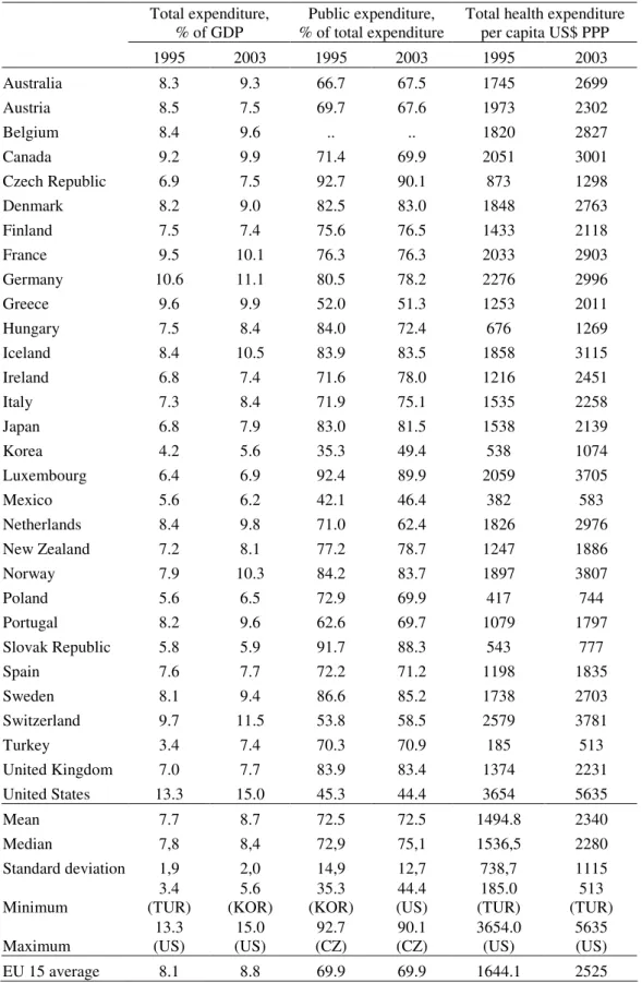
Health is one of the most important services provided by governments in almost every country. According to OECD (2005), OECD countries expended an average of 8.7 per cent of GDP in 2003 on health institutions, of which 6.3 per cent of GDP were from public sources. In a general sense, health provision is efficient if its producers make

the best possible use of available inputs, and the sole fact that health inputs weight heavily on the public purse would call for a careful efficiency analysis. A health system not being efficient would mean either that results (or “outputs”) could be increased without spending more, or else that expense could actually be reduced without affecting the outputs, provided that more efficiency is assured. Research results presented here indicate that there are cases where considerable improvements can be made in this respect.

The fact of health spending being predominantly public is particularly true notably in OECD countries. Table 1 summarises some relevant data for thirty OECD countries concerning health spending. For instance, public expenditure as a share of total spending averaged 72.5 per cent in 2003, ranging from 44.4 per cent in the USA to 90.1 per cent in the Czech Republic. For the EU15, average total spending was 8.8 per cent of GDP in 2003, which is close to the OECD value, slightly up from the 8.1 per cent ratio observed in 1995. On the other hand, average public expenditure as a share of total expenditure in health was, in 2003, lower in the EU15 than in the OECD, the corresponding ratios being equal to 69.9 and 72.5 percent, respectively. Furthermore, data reported in Table 1 show that total per capita health spending is very diverse across OECD countries. Indeed, the country that spends more on health in per capita terms, the USA, expends more than two times the OECD average and eleven times

more than the country that spends the least, Turkey, even though the per capita GDP ratio between those two countries is roughly five and a half.

Moreover, the relevance of assessing the quality of public spending and redirecting it to more growth enhancing items is stressed, for instance, in EC (2004) as being an important goal for governments to pursue. Internationally, there is a shift in the focus of the analysis from the amount of public resources used by a government, to services delivered, and also to achieved outcomes and their quality (see OECD, 2003).

In our research, we measure and compare health output across countries using precisely the abovementioned type of quality measures – we resort to the most recent cross-nationally comparable evidence on health variables, as reported in OECD (2005).

Previous research on the international comparative performance of the public sector in general and of health outcomes in particular, including Afonso, Schuknecht and Tanzi (2005) for public expenditure in the OECD, and Gupta and Verhoeven (2001) for education and health in Africa, has already suggested that important inefficiencies are at work. These studies use free disposable hull analysis (FDH) with inputs measured in monetary terms. Spinks and Hollingsworth (2005) assess health efficiency for OECD countries using DEA based Malmquist indexes. They report a mean value of 0.961 for an OECD dataset suggesting that overall, member countries have moved slightly away from the frontier, implying a decrease in technical efficiency, between 1995 and 2000. Using both FDH and DEA analysis, Afonso and St. Aubyn (2005) studied efficiency in providing health and education in OECD countries using physically measured inputs and concluded that if all countries were efficient, input usage could be reduced by about 13 per cent without affecting output. Using a more extended sample Evans et al. (2000) evaluate the efficiency of health expenditure in 191 countries using a parametric methodology. In addition, Afonso and St. Aubyn

(2006) also used a two-step approach for education performance in OECD countries.

DEA jargon.3 They are, however, of a fundamentally different nature from input variables, in so far as their values cannot be changed in a meaningful spell of time by the DMU, here a country.

3. Analytical methodology

3.1. DEA framework

DEA, which assumes the existence of a convex production frontier, allows the calculation of technical efficiency measures that can be either input or output oriented. The purpose of an output-oriented study is to evaluate by how much output quantities can be proportionally increased without changing the input quantities used. This is the perspective taken in this paper. Note, however, that one could also try to assess by how much input quantities can be reduced without varying the output. Both output and input-oriented models will identify the same set of efficient/inefficient producers or DMUs.4

The description of the linear programming problem to be solved, output oriented and assuming variable returns to scale hypothesis, is sketched below. Suppose there are p

inputs and q outputs for n DMUs. For the i-th DMU, yi is the column vector of the

outputs and xi is the column vector of the inputs. We can also define X as the (p×n)

input matrix and Y as the (q×n) output matrix. The DEA model is then specified with the following mathematical programming problem, for a given i-th DMU:

0 1 ' 1 to s. , ≥ = ≥ ≤ λ λ λ λ δ δ δ λ n X x Y y Max i i i i i

. (1)

3 Throughout the paper we use interchangeably the terms “non-discretionary”, “exogenous” and “environmental” when qualifying variables or factors not initially considered in the DEA programme.

4

In problem (1), δi is a scalar satisfyingδi ≥1, more specifically it is the efficiency

score that measures technical efficiency of the i-th unit as the distance to the efficiency frontier, the latter being defined as a linear combination of best practice

observations. Withδ_i >1, the decision unit is inside the frontier (i.e. it is inefficient),

while δ_i =1 implies that the decision unit is on the frontier (i.e. it is efficient). The

vector λ is a (n×1) vector of constants that measures the weights used to compute the location of an inefficient DMU if it were to become efficient.

3.2. Non-discretionary inputs and the DEA/Tobit two-steps procedure

The standard DEA models as the one described in (1) incorporate only discretionary

inputs, those whose quantities can be changed at the DMU will, and do not take into account the presence of environmental variables or factors, also known as

non-discretionary inputs. However, socio-economic differences may play a relevant role in determining heterogeneity across DMUs – either schools, hospitals or countries’ achievements in an international comparison – and influence outcomes. In what health is concerned, these exogenous socio-economic factors can include, for instance, household wealth, eating habits and education level.

As non-discretionary and discretionary inputs jointly contribute to each DMU outputs, there are in the literature several proposals on how to deal with this issue, implying usually the use of two-stage and even three-stage models.5

Let zi be a (1×r) vector of non-discretionary outputs. In a typical two-stage approach,

the following regression is estimated:

i i i

z

β

ε

δ

ˆ

=

+

where δˆ is the efficiency score that resulted from stage one, i.e. from solving (1). _i β is

a (r×1) vector of parameters to be estimated in step two associated with each

5

considered non-discretionary input. The fact that δˆ_i ≥1 has led many researchers to

estimate (2) using censored regression techniques (Tobit), although others have used OLS.6

Figure 1 illustrates the basic idea behind a two-stage approach. In a simplified one output and one input DEA problem, A, B and C are found to be efficient, while D is an inefficient DMU. The output score for unit D equals (d1+d2)/d1, and is higher than

one. However, unit D inefficiency may be partly ascribed to a “harsh environment” – a number of perturbing environmental factors may imply that unit D produces less than the theoretical maximum, even if discretionary inputs are efficiently used. In our example, and if the environment for unit D was more favourable (e. g. similar to the sample average), then we would have observed Dc. In other words, unit D would have

produced more and would be nearer the production possibility. The environment corrected output score would be (d1c+d2c)/d1c, lower than (d1+d2)/d1, and closer to

unity.

[Insert Figure 1 here]

3.3. Non-discretionary inputs and bootstrap

The two-stage DEA/Tobit method is likely to be biased in small samples for two reasons. Firstly, the fact that output scores are jointly estimated by DEA implies that

the error term εi in equation (2) is serially correlated. Secondly, non-discretionary

variables zi are correlated to the error term εI. This derives from the fact that

non-discretionary inputs are correlated to the outputs, and therefore to estimated efficiency scores.

To surmount this, Simar and Wilson (2007) propose two alternatives based on bootstrap methods7. Similarly to the DEA/Tobit procedure, the efficiency score

6

See Simar and Wilson (2007) for an extensive list of published examples of the two step approach.

7

depends linearly on the environmental variables, but the error term is a truncated, and not censored, normal random variable8.

The first bootstrap method (“algorithm 1”) implies the estimation of the efficiency scores using DEA, as in the DEA/Tobit analysis. However, the influence of non-discretionary inputs on efficiency is estimated by means of a truncated linear

regression. Coefficient significance is then assessed by bootstrapping. We have considered 2000 bootstrap estimates for that effect.

The scores derived from DEA are biased towards 1 in small samples. Simar and Wilson (2007) second bootstrap procedure, “algorithm 2”, includes a parametric bootstrap in the first stage problem, so that bias-corrected estimates for the efficiency scores are produced. These corrected scores replace the DEA original ones, and estimation of environment effects proceeds like in algorithm 1.

4. Empirical analysis

4.1. Data and indicators

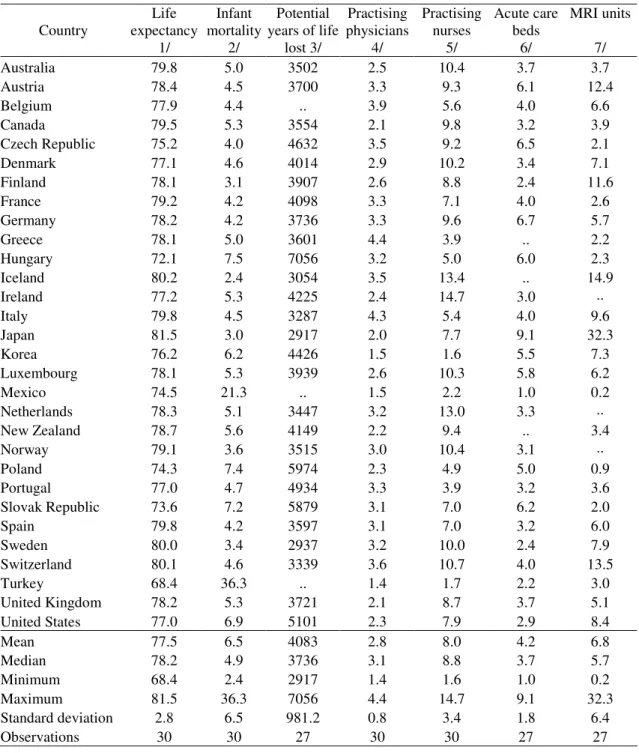
OECD (2005) is our chosen health database for OECD countries.9 _{Typical input}

variables include medical technology indicators and health employment. Output is to be measured by indicators such as life expectancy and infant mortality, in order to assess potential years of added life.

It is of course difficult to measure something as complex as the health status of a population. We have not innovated here, and took two usual measures of health

attainment, infant mortality and life expectancy.10

8

We implemented these algorithms in Matlab. Programmes and functions are available on request.

9

The data and the sources used in the paper are presented in the Annex.

10

Efficiency measurement techniques used in this paper imply that outputs are measured in such a way that “more is better.” This is clearly not the case with infant mortality. Recall that the Infant Mortality Rate (IMR) is equal to:

(Number of children who died before 12 months)/(Number of born children)×1000.

We have calculated an “Infant Survival Rate”, ISR,

IMR IMR

ISR=1000− , (2)

which has two nice properties: it is directly interpretable as the ratio of children that survived the first year to the number of children that died; and, of course, it increases with a better health status.

We have considered a third output measure, which we call Potential Years of Life Not

Lost, PYLNL. This variable was computed on the basis of the indicator Potential Years of Life Lost, PYLL, reported by OECD (2005). This last variable, PYLL, equals the number of life years lost due to all causes before the age of 70 and that could be, a priori, prevented. Therefore, and for our subsequent DEA analysis, and similarly to the Infant Mortality Rate, a transformation had to be done, in order to provide an increasing monotonic relation between the variable, number of years not lost, and health status.

Our transformed variable is:

-PYNLL=

λ

where λ=3 618 010 is an estimate of the number of potential years of life for a population under 70 years.11

11

Therefore, our frontier model for health is based upon three output variables:

- the infant survival rate, - and life expectancy,

- potential years of life not lost.

We compare physically measured inputs to outcomes. Quantitative inputs are the

number of practising physicians, practising nurses, acute care beds per thousand habitants and high-tech diagnostic medical equipment, specifically magnetic resonance imagers (MRI).12 Table 2 reports the relevant statistics for the set of OECD countries.

[Insert Table 2 here]

From Table 2 one notices that practising nurses per one thousand persons, in the period 2000–2003, ranged from 1.6 in Korea to 14.7 in Ireland. For the same period there was also a high range of practising physicians per one thousand persons, from 1.4–1.5 in Turkey and in Korea to 4.3–4.4 in Italy and in Greece. Additionally, the number of MRI per million persons ranged from 0.2 in Mexico to 32.2 in Japan, and the hospital acute care beds per one thousand persons ranged from 1.0 in Mexico to 9.1 in Japan.

Table 2 also shows that for the period 2000–2003 life expectancy at birth ranged form 68.4 years in Turkey to 81.5 in Japan, and infant mortality ranged form 2.4 in Iceland to 36.3 in Turkey. In addition, the potential years of life not lost per 100000 population was 73 per cent above the average in Hungary and 29 per cent below average in Japan.

4.2. Principal component analysis

In order to go around the eventual difficulties posed to the DEA approach when there are a significant number of inputs and/or outputs, we used principal component analysis (PCA) to aggregate some of the indicators. The use of PCA reduces the

12

dimensionality of multivariate data, which is what we have regarding health status, and the health care resources used.

The idea of PCA is to describe the variation of a multivariate data set through linear combinations of the original variables (see, for instance, Everitt and Dunn, 2001). Generally, we are interested in seeing if the first few components portray most of the

variation of the original data set, for instance, 80 per cent or 90 per cent, without much loss of information. In a nutshell, the principal components are uncorrelated linear combinations of the original variables, which are then ranked by their variances in descending order. This provides a more parsimonious representation of the data set and avoids that in the DEA computations too many DMUs are labelled efficient by default.

Usually one applies PCA by imposing that the original variables are normalized to have zero mean. This means that the computed principal components scores also have zero mean, and therefore some of the results from PCA are negative. Since DEA inputs and outputs need to be strictly positive, PCA results will be increased by the most negative value in absolute value plus one, in order to ensure strictly positive data (see, for instance, Adler and Golany, 2001).

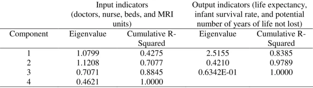
We applied PCA to the four input variables, doctors, nurses, beds and MRI units. The results of such analysis (see Table 3) led us to use the first three principal components as the three input measures, which explain around 88 per cent of the variation of the four variables. This also implies that we only take into account the components whose associated eigenvalues are above 0.7, a rule suggested by Jollife (1972).

Applying PCA also to the set of our selected output variables, life expectancy, infant survival rate and potential number of years of life not lost, we selected the first principal component as the output measure since it accounts for around 84 per cent of the variation of the three variables (see Table 3).

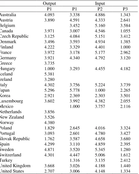
We report in Table 4 the abovementioned principal components, to be used in the subsequent section in DEA computations.

[Insert Table 4 here]

4.3. DEA efficiency results

In Table 5 we report results for the standard DEA variable-returns-to-scale technical efficiency output scores and peers of each of the considered countries. The specification used includes as inputs the first three components of the PCA performed to the base variables doctors, nurses, beds and MRI units. As output we use the first component of the PCA applied to the base variables infant survival rate, life expectancy, and potential years of life not lost, as explained in the previous section.

[Insert Table 5 here]

It is possible to observe in Table 5 that seven countries would be located on the theoretical production possibility frontier with the standard DEA approach: Canada, Finland, Japan, Korea, Spain, Sweden and the USA13.Canada, Finland, Japan, Spain and Sweden are located in the efficient frontier because they perform quite well in the output indicator, getting above average results. On the other hand, Korea and the USA are generally below average regarding the use of resources in all the first three components selected. Another set of three countries is located on the opposite end – Hungary, the Slovak Republic and Poland. DEA analysis indicates that their output could be substantially increased if they were to become located on the efficiency frontier. On average and as a conservative estimate, countries could have increased

their results by 40 per cent using the same resources.

13

4.4. Explaining inefficiency – the role of non-discretionary inputs

Using the DEA efficiency scores computed in the previous subsection, we now evaluate the importance of non-discretionary inputs. We present results both from Tobit regressions and bootstrap algorithms. Even if Tobit results are possibly biased, it is not clear that bootstrap estimates are necessarily more reliable. In fact, the latter

are based on a set of assumptions concerning the data generation process and the perturbation term distribution that may be disputed. Taking the pros and cons of both methods into account, it seems sensible to apply both of them. If outcomes are comparable, this adds robustness and confidence to the results we are interested in.

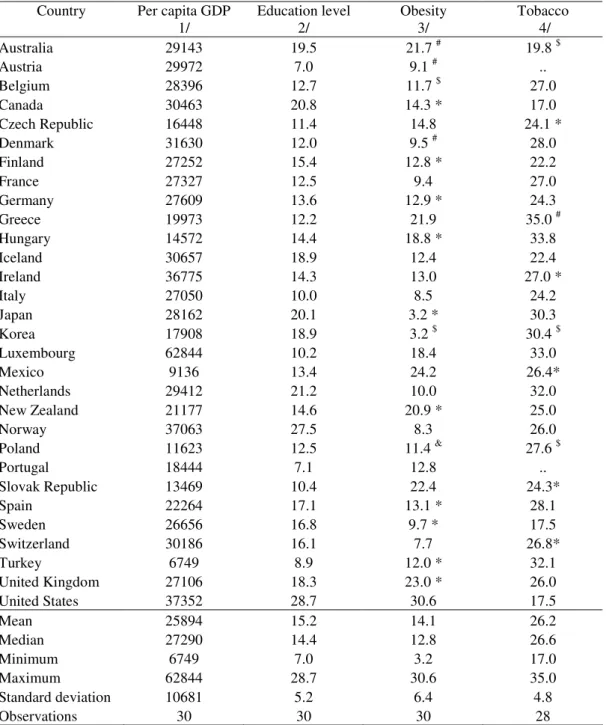
In order to explain the efficiency scores, we regress them on GDP per capita, Y, educational level, E, obesity, O, and tobacco consumpion, T, as follows14

0 1 2 3 4

ˆ

i Yi Ei Oi Ti i

δ

β

β

β

β

β

ε

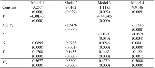
We first report in Table 6 results from the censored normal Tobit regressions for several alternative specifications of equation (4).

[Insert Table 6 here]

Inefficiency in the health sector is strongly related to the four variables that are, at least in the short to medium run, beyond the control of governments: the economic

background, proxied here by the country GDP per capita, the level of education, smoking habits, and obesity. The estimated coefficients of the first two non-discretionary inputs are statistically significant and negatively related to the efficiency measure. For instance, an increase in education achievement reduces the efficiency score, implying that the relevant DMU moves closer to the theoretical production possibility frontier. Therefore, the better the level of education, the higher the efficiency of health provision in a given country. The same reasoning applies to GDP,

14

with higher GDP per capita resulting in more efficiency. On the other hand, efficiency is lower the stronger smoking habits are and the higher the percentage of obese population is.

We also considered other variables as non-discretionary inputs: income inequality via the Gini coefficient, the ratio of public-to-total expenditure in health, spending on pharmaceuticals as a percentage of health expenditure, percentage of population over 65 years, per capita alcohol and sugar consumption, and total calories intake. However, none of these variables prove to be statistically significant and the

estimation results are not reported for the sake of space.

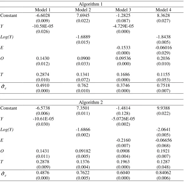
Table 7 reports the estimation results from the bootstrap procedures employing algorithms 1 and 2, as described in sub-section 3.3. Estimated coefficients are very similar irrespective of the algorithm used to estimate them. Moreover, they are also close to the estimates derived from the more usual Tobit procedure, and, very importantly, they are highly significant.

[Insert Table 7 here]

Significance across different model formulations and estimation methods is important and robust empirical evidence that efficiency in health depends directly on a country’s wealth and on education levels, and inversely on tobacco consumption and obesity. In a nutshell, population of poorer countries where education levels are low tend to under perform, so that results are further away from the efficiency frontier. The same reasoning applies to the other two environmental factors, with higher smoking habits and obesity levels drawing countries away from health related efficient performance.

Equation (4) can be regarded as a decomposition of the output efficiency score into two distinct parts:

– the one that is the result ofIn all methods and models a country’s

– the one that includes all other factors that have an influence on efficiency, including therefore inefficiencies associated with the health system itself, and given

by εt.

In all methods and models, models 1, 3 and 4 provide the best fit (as can be seen by

the lower estimated standard deviation of ε). We choose models 1 and 3 for our

exercise of correcting for environmental variables in order to use versions with and without education as an exogenous factor.

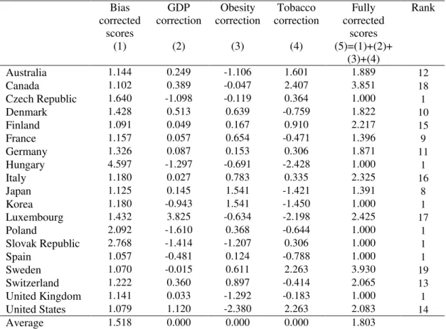
The first column in Table 8 includes the bias corrected scores for Model 1, the one with the best fit using bootstrap algorithms (as can be seen by the lower estimated

standard deviation of ε). Algorithm 2 implies a bias correction after estimating output

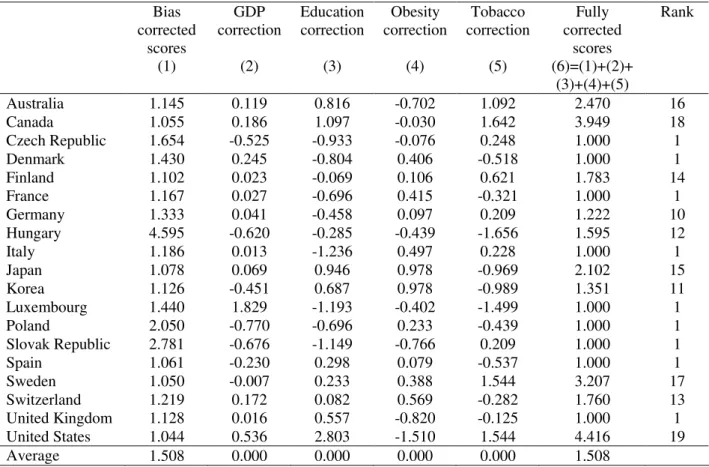
efficiency scores, taking into account the correlation between these scores and the environmental variables. We also present score corrections for the three environmental variables. GDP, obesity, and tobacco consumption corrections were computed as the changes in scores by artificially considering that Y, O, and T varied to the sample average in each country. Fully corrected scores, presented in column five, are estimates of output scores purged from environmental effects and result from the summation of the previous four columns, truncated to one when necessary.

[Insert Table 8 here]

Comparing the ranks in the last column of Table 8, resulting from corrections for both bias and environmental variables, with the previously presented ranking from the standard DEA analysis (see Table 5 above), it is apparent that significant changes

occurred. For the purpose of such comparison one should notice that the number of countries considered dropped from twenty-one in the DEA calculations to nineteen in the two-step analysis, since tobacco consumption data was not available for Austria and Portugal.

relative position after taking into account environmental variables, namely Canada, Sweden, and the US, and to less a extent, Japan. At last, countries like Korea and Spain keep their good positioning.

Additionally, by looking at GDP, obesity and tobacco consumption corrections in Table 8, it is apparent that in some countries, environmental “harshness” essentially

results from low GDP per head, as in the Czech Republic, Korea, Poland and Spain. For instance, for the US, lower than average tobacco consumption is offset by above average obesity, while for Japan, Korea, Luxembourg, and Switzerland we see an opposite pattern. Finally, note that in countries like Germany and Italy, all three environmental variables push down performance, while an inverse result can be observed for Hungary.

Alternatively, a similar analysis can be conducted for Model 3, where we now have four environmental variables: GDP, education, obesity, and tobacco consumption (see Table 9).

[Insert Table 9 here]

From the results in Table 9 it is possible to conclude that education correction is not beneficial for countries such as Canada, the US, Japan or Korea. Indeed, and as results from both Tobit and bootstrap analysis indicate, the percentage of population with tertiary education is a relevant exogenous variable in explaining health efficiency scores. On the other hand, the below average results in this variable for several other countries, such as the Czech Republic, Italy and Luxembourg, allow for an improvement in their efficiency rankings after making the corrections related to all

four non-discretionary factors used in Model 3.

5. Conclusion

obesity). In methodological terms, we have employed a two-stage semi-parametric procedure. Firstly, output efficiency scores were estimated by solving a standard DEA problem with countries as DMUs. Secondly, these scores were explained in a regression with the environmental variables as independent variables.

Results from the first-stage imply that inefficiencies may be quite high. On average

and as a conservative estimate, countries could have increased their results by 40 per cent using the same resources. Countries like Hungary, the Slovak Republic and Poland display significant room for improvement.

The fact that a country is seen as far away from the efficiency frontier is not necessarily a result of inefficiencies engendered within the health system. Our second stage procedures shows that GDP per head, educational attainment, tobacco consumption, and obesity are highly and significantly correlated to output scores – a wealthier and more cultivated environment are important conditions for a better health performance, while a more obese population and prevalence of smoking habits worsen health performance. Moreover, it becomes possible to correct output scores by considering the harshness of the environment where the health system operates. Country rankings and output scores derived from this correction can be substantially different from standard DEA results.

Non-discretionary outputs considered here cannot be changed in the short run. For example, educational attainment is essentially given in the coming year. However, contemporaneous educational and social policy will have an impact on future educational attainment. A similar reasoning applies to smoking habits, which are difficult to change, but where, for instance, tax measures are usually considered and

implemented by the governments. Obesity problems also impinge negatively on the performance of the health system, and may be related to cultural traditions.

Appendix

In this appendix we explain the derivation of the output variable Potential Years of Life Not Lost. According to OECD (2005), the variable Potential Years of Life Lost per 100 000 population is given by:

100000 ) ( 1 0 × − = − = n a l a at at t P P p d a l

PYLL , (A1)

where l, the age limit, was set to 70 years, dat is the number of deaths at age a at year t

and pat is the number of persons aged a at year t. Pa and Pn are, respectively, the

number of persons aged a and the total number of persons in the reference population, the OECD total population in 1980.

Our relevant variable, Potential Years of Life Not Lost, PYLNL, is defined by us as follows: 100000 ) ( 1 0 × − − = − = n a l a at at at t P P p d p a l

PYLNL . (A2)

Note that pat - dat equals the number of persons aged a at year t that did not die.

Equation (A2) is equivalent to:

100000 ) ( 100000 ) ( 1 0 1 0 × − − × − = − = − = n a l a at at n a l a t P P p d a l P P a l

PYLNL , (A3)

where the second term of the difference in the right-hand side is simply PYLL. The first term of the right-hand side of (A3) was computed by us via the very same population structure in 1980 used and reported by OECD (2005) when calculating the

PYLL. It gives (see equation (3) in the text):

PYLL

PYNLL=3618010- , (A4)

References

Adler, N. and Golany, B. (2001). “Evaluation of deregulated airline networks using data envelopment analysis combined with principal component analysis with an application to Western Europe”. European Journal of Operational Research, 132, 260-273.

Afonso, A.; Schuknecht, L. and Tanzi, V. (2005). “Public Sector Efficiency: An International Comparison,” Public Choice, 123 (3-4), 321-347.

Afonso, A. and St. Aubyn (2005). “Non-parametric Approaches to Education and Health Efficiency in OECD Countries,” Journal of Applied Economics, 8 (2), 227-246.

Afonso, A. and St. Aubyn (2006). “Cross-country Efficiency of Secondary Education Provision: a Semi-parametric Analysis with Non-discretionary Inputs,” Economic

Modelling, 23 (3), 476-491.

Charnes, A.; Cooper, W. and Rhodes, E. (1978). “Measuring the efficiency of decision making units,” European Journal of Operational Research, 2 (6), 429–444.

Coelli, T.; Rao, P., O’Donnell, C. and Battese, G. (2005). An Introduction to

Efficiency and Productivity Analysis. Kluwer, Boston.

EC (2004). Public Finances in EMU - 2004. A report by the Commission services, SEC(2004) 761. Brussels.

Evans, D.; Tandon, A.; Murray, C. and Lauer, J. (2000). “The Comparative Efficiency of National Health Systems in Producing Health: an Analysis of 191 Countries”, GPE Discussion Paper Series 29, Geneva, World Health Organisation.

Everitt, B. and Dunn, G. (2001). Applied Multivariate Data analysis, 2nd edition, Arnold, London.

Farrell, M. (1957). “The Measurement of Productive Efficiency,” Journal of the Royal Statistical Society, Series A, 120, Part 3, 253-290.

Gupta, S. and Verhoeven, M. (2001). “The Efficiency of Government Expenditure – Experiences from Africa", Journal of Policy Modelling, 23, 433-467.

Jollife, I. (1972) “Discarding variables in a principal component analysis 1: Artificial data”, Applied Statistics, 21, 160-173.

OECD (2003). “Enhancing the Cost Effectiveness of Public Spending,” in Economic

Outlook, vol. 2003/02, n. 74, December, OECD.

OECD (2005), OECD Health Data 2005, Paris, OECD.

Ruggiero, J. (2004). “Performance evaluation when non-discretionary factors correlate with technical efficiency”, European Journal of Operational Research 159, 250–257.

Simar, L. and Wilson, P. (2000). “A General Methodology for Bootstrapping in Nonparametric Frontier Models”, Journal of Applied Statistics 27, 779-802.

Simar, L. and Wilson, P. (2007). “Estimation and Inference in Two-Stage, Semi-Parametric Models of Production Processes”, Journal of Econometrics 136 (1), 31-64.

Spinks, J. and Hollingsworth, B. (2005). “Health production and the socioeconomic determinants of health in OECD countries: the use of efficiency models”, Monash University, Center for Health Economics, Working Paper 151.

Thanassoulis, E. (2001). Introduction to the Theory and Application of Data

Annex – Data and sources

Table A1. Health indicators

Country Life expectancy 1/ Infant mortality 2/ Potential years of life

lost 3/ Practising physicians 4/ Practising nurses 5/ Acute care beds 6/ MRI units 7/ Australia 79.8 5.0 3502 2.5 10.4 3.7 3.7 Austria 78.4 4.5 3700 3.3 9.3 6.1 12.4 Belgium 77.9 4.4 .. 3.9 5.6 4.0 6.6 Canada 79.5 5.3 3554 2.1 9.8 3.2 3.9 Czech Republic 75.2 4.0 4632 3.5 9.2 6.5 2.1 Denmark 77.1 4.6 4014 2.9 10.2 3.4 7.1 Finland 78.1 3.1 3907 2.6 8.8 2.4 11.6 France 79.2 4.2 4098 3.3 7.1 4.0 2.6 Germany 78.2 4.2 3736 3.3 9.6 6.7 5.7 Greece 78.1 5.0 3601 4.4 3.9 .. 2.2 Hungary 72.1 7.5 7056 3.2 5.0 6.0 2.3 Iceland 80.2 2.4 3054 3.5 13.4 .. 14.9 Ireland 77.2 5.3 4225 2.4 14.7 3.0 .. Italy 79.8 4.5 3287 4.3 5.4 4.0 9.6 Japan 81.5 3.0 2917 2.0 7.7 9.1 32.3 Korea 76.2 6.2 4426 1.5 1.6 5.5 7.3 Luxembourg 78.1 5.3 3939 2.6 10.3 5.8 6.2 Mexico 74.5 21.3 .. 1.5 2.2 1.0 0.2 Netherlands 78.3 5.1 3447 3.2 13.0 3.3 .. New Zealand 78.7 5.6 4149 2.2 9.4 .. 3.4 Norway 79.1 3.6 3515 3.0 10.4 3.1 .. Poland 74.3 7.4 5974 2.3 4.9 5.0 0.9 Portugal 77.0 4.7 4934 3.3 3.9 3.2 3.6 Slovak Republic 73.6 7.2 5879 3.1 7.0 6.2 2.0 Spain 79.8 4.2 3597 3.1 7.0 3.2 6.0 Sweden 80.0 3.4 2937 3.2 10.0 2.4 7.9 Switzerland 80.1 4.6 3339 3.6 10.7 4.0 13.5 Turkey 68.4 36.3 .. 1.4 1.7 2.2 3.0 United Kingdom 78.2 5.3 3721 2.1 8.7 3.7 5.1 United States 77.0 6.9 5101 2.3 7.9 2.9 8.4 Mean 77.5 6.5 4083 2.8 8.0 4.2 6.8 Median 78.2 4.9 3736 3.1 8.8 3.7 5.7 Minimum 68.4 2.4 2917 1.4 1.6 1.0 0.2 Maximum 81.5 36.3 7056 4.4 14.7 9.1 32.3 Standard deviation 2.8 6.5 981.2 0.8 3.4 1.8 6.4 Observations 30 30 27 30 30 27 27

1/ Years of life expectancy, total population at birth. Average for 2000 and 2003. Source: OECD (2005).

2/ Deaths per 1000 live births. Average for 2000-2003. Source: OECD (2005). 3/All causes - <70 year,/100 000. Average for 2000-2003. Source: OECD (2005). 4/ 5/ 6/ Density per 1000 population. Average for 2000-2003. Source: OECD (2005). 7/ Per million population. Average for 2000-2003. Source: OECD (2005).

Table A2. Non-discretionary factors

Country Per capita GDP 1/

Education level 2/

Obesity 3/

Tobacco 4/ Australia 29143 19.5 21.7 # 19.8 $ Austria 29972 7.0 9.1 # .. Belgium 28396 12.7 11.7 $ 27.0 Canada 30463 20.8 14.3 * 17.0 Czech Republic 16448 11.4 14.8 24.1 * Denmark 31630 12.0 9.5 # 28.0 Finland 27252 15.4 12.8 * 22.2 France 27327 12.5 9.4 27.0 Germany 27609 13.6 12.9 * 24.3 Greece 19973 12.2 21.9 35.0 # Hungary 14572 14.4 18.8 * 33.8 Iceland 30657 18.9 12.4 22.4 Ireland 36775 14.3 13.0 27.0 * Italy 27050 10.0 8.5 24.2 Japan 28162 20.1 3.2 * 30.3 Korea 17908 18.9 3.2 $ 30.4 $ Luxembourg 62844 10.2 18.4 33.0 Mexico 9136 13.4 24.2 26.4* Netherlands 29412 21.2 10.0 32.0 New Zealand 21177 14.6 20.9 * 25.0 Norway 37063 27.5 8.3 26.0 Poland 11623 12.5 11.4 & 27.6 $ Portugal 18444 7.1 12.8 .. Slovak Republic 13469 10.4 22.4 24.3* Spain 22264 17.1 13.1 * 28.1 Sweden 26656 16.8 9.7 * 17.5 Switzerland 30186 16.1 7.7 26.8* Turkey 6749 8.9 12.0 * 32.1 United Kingdom 27106 18.3 23.0 * 26.0 United States 37352 28.7 30.6 17.5 Mean 25894 15.2 14.1 26.2 Median 27290 14.4 12.8 26.6 Minimum 6749 7.0 3.2 17.0 Maximum 62844 28.7 30.6 35.0 Standard deviation 10681 5.2 6.4 4.8 Observations 30 30 30 28

1/ GDP per capita - (USD) PPP GDP and population in 2003. Source: World Development Indicators Database, September 2003.

2/ Percentage of population at ISCED 5A = Programmes at the tertiary level equivalent to university programmes (ISCED-76: level 6), andISCED 6 = Advanced research programmes at the tertiary level, equivalent to PhD programmes. (ISCED-76: level 7). Average for 2000-2003. Source: OECD, Education at a Glance 2005, www.oecd.org/edu/eag2005.

3/ 2002 body weight, obese population (BMI>30kg/m2). Source: OECD HEALTH DATA 2005, Sept. 05. * - 2003; $ - 2001; # 1999; & - 1996.

4/ Tobacco consumption (% of pop), 2003. Source: OECD HEALTH DATA 2005, Sept. 05. * - 2002; $ - 2001; # 2000.

Tables and figures

Table 1 – Public and total expenditure on health

Total expenditure, % of GDP

Public expenditure, % of total expenditure

Total health expenditure per capita US$ PPP 1995 2003 1995 2003 1995 2003 Australia 8.3 9.3 66.7 67.5 1745 2699 Austria 8.5 7.5 69.7 67.6 1973 2302 Belgium 8.4 9.6 .. .. 1820 2827 Canada 9.2 9.9 71.4 69.9 2051 3001 Czech Republic 6.9 7.5 92.7 90.1 873 1298 Denmark 8.2 9.0 82.5 83.0 1848 2763 Finland 7.5 7.4 75.6 76.5 1433 2118 France 9.5 10.1 76.3 76.3 2033 2903 Germany 10.6 11.1 80.5 78.2 2276 2996 Greece 9.6 9.9 52.0 51.3 1253 2011 Hungary 7.5 8.4 84.0 72.4 676 1269 Iceland 8.4 10.5 83.9 83.5 1858 3115 Ireland 6.8 7.4 71.6 78.0 1216 2451 Italy 7.3 8.4 71.9 75.1 1535 2258 Japan 6.8 7.9 83.0 81.5 1538 2139 Korea 4.2 5.6 35.3 49.4 538 1074 Luxembourg 6.4 6.9 92.4 89.9 2059 3705 Mexico 5.6 6.2 42.1 46.4 382 583 Netherlands 8.4 9.8 71.0 62.4 1826 2976 New Zealand 7.2 8.1 77.2 78.7 1247 1886 Norway 7.9 10.3 84.2 83.7 1897 3807 Poland 5.6 6.5 72.9 69.9 417 744 Portugal 8.2 9.6 62.6 69.7 1079 1797 Slovak Republic 5.8 5.9 91.7 88.3 543 777 Spain 7.6 7.7 72.2 71.2 1198 1835 Sweden 8.1 9.4 86.6 85.2 1738 2703 Switzerland 9.7 11.5 53.8 58.5 2579 3781 Turkey 3.4 7.4 70.3 70.9 185 513 United Kingdom 7.0 7.7 83.9 83.4 1374 2231 United States 13.3 15.0 45.3 44.4 3654 5635 Mean 7.7 8.7 72.5 72.5 1494.8 2340 Median 7,8 8,4 72,9 75,1 1536,5 2280 Standard deviation 1,9 2,0 14,9 12,7 738,7 1115 Minimum 3.4 (TUR) 5.6 (KOR) 35.3 (KOR) 44.4 (US) 185.0 (TUR) 513 (TUR) Maximum 13.3 (US) 15.0 (US) 92.7 (CZ) 90.1 (CZ) 3654.0 (US) 5635 (US) EU 15 average 8.1 8.8 69.9 69.9 1644.1 2525 Sources: OECD Health Data 2005 - Frequently asked data

Table 2 – Summary statistics of the input and output data

Mean Standard

deviation

Minimum Maximum

Life expectancy (in years) 1/ 77.5 2.8 68.4

(TUR)

81.5 (JAP) Infant mortality rate (deaths per

1000 live births) 2/

4.5 6.5 2.4

(ICE)

36.3 (TUR) Potential years of life lost (All

causes - <70 year,/100 000) 2/

4083 981.2 2917

(JAP)

7056 (HU) Practising physicians,density per

1000 population 2/

2.8 0.8 1.4

(TUR)

4.4 (GRC)

Practising nurses,density per 1000

population 2/

8.0 3.4 1.6

(KOR)

14.7 (IRE) Acute care beds, density per 1000

population 2/

4.2 1.8 1.0

(MEX)

9.1 (JAP) MRI units, per million population

2/

6.8 6.4 0.2

(MEX)

32.3 (JAP)

Notes: 1/ Average for 2000 and 2003. 2/ Average for 2000-2003.

TUR – Turkey; JAP – Japan; ICE – Iceland; HU – Hungary; GCR – Greece; KOR – Korea; IRE – Ireland; MEX – Mexico.

Table 3 – Eigenvalues and cumulative R-squared of PCA on health input and output indicators

Input indicators (doctors, nurse, beds, and MRI

units)

Output indicators (life expectancy, infant survival rate, and potential

number of years of life not lost)

Component Eigenvalue Cumulative

R-Squared

Eigenvalue Cumulative

R-Squared

1 1.0799 0.4275 2.5155 0.8385

2 1.1208 0.7077 0.4210 0.9789

3 0.7071 0.8845 0.6342E-01 1.0000

Table 4 – Principal components used in the DEA calculations

Output Input

P1 P1 P2 P3

Australia 4.093 3.338 4.886 1.343

Austria 3.890 4.591 4.333 2.641

Belgium 3.452 5.160 3.584

Canada 3.971 3.007 4.546 1.055

Czech Republic 3.125 4.084 5.151 3.412

Denmark 3.496 3.593 4.934 1.385

Finland 4.222 3.329 4.401 1.000

France 3.972 3.178 5.177 2.962

Germany 3.921 4.340 4.792 3.120

Greece 3.735

Hungary 1.000 3.293 4.455 4.182

Iceland 5.381

Ireland 3.280

Italy 4.302 3.756 5.224 3.739

Japan 5.296 5.778 1.000 2.265

Korea 2.921 2.369 2.303 3.501

Luxembourg 3.602 3.992 4.382 2.055

Mexico 1.000 3.757 2.116

Netherlands 3.856

New Zealand 3.526

Norway 4.380

Poland 1.829 2.645 4.016 3.324

Portugal 3.093 2.601 4.780 3.427

Slovak Republic 1.762 3.587 4.658 3.680

Spain 4.299 3.110 4.859 2.395

Sweden 4.871 3.520 5.345 1.280

Switzerland 4.301 4.447 5.006 1.612

Turkey 1.316 3.135 2.412

United Kingdom 3.668 3.026 4.188 1.440

United States 2.707 3.006 4.148 1.334

Table 5 – DEA output efficiency results for health efficiency in OECD countries, 3 inputs (PCA on doctors, nurses, beds and MRI) and 1 output (PCA on life expectancy, infant survival rate, and potential number of years of life not lost)

Country VRS TE Rank Peers Rank 2

Australia 1.101 10 Canada, Sweden, Korea, Finland 10

Austria 1.304 15 Sweden, Japan 15

Canada 1.000 1 Canada 6

Czech Republic 1.592 18 Japan, Sweden 18

Denmark 1.368 16 Korea, Japan, Sweden, Finland 16

Finland 1.000 1 Finland 4

France 1.106 11 Sweden, Spain 11

Germany 1.282 14 Sweden, Japan 14

Hungary 4.386 21 Sweden, Japan, Korea 21

Italy 1.143 12 Sweden, Japan 12

Japan 1.000 1 Japan 2

Korea 1.000 1 Korea 3

Luxembourg 1.372 17 Korea, Japan, Sweden 17

Poland 1.876 19 Spain, Korea 19

Portugal 1.083 9 Korea, Spain 9

Slovak Republic 2.667 20 Korea, Sweden, Japan 20

Spain 1.000 1 Spain 4

Sweden 1.000 1 Sweden 1

Switzerland 1.166 13 Sweden, Japan 13

United Kingdom 1.070 8 Canada, Sweden, Korea, Finland 8

United States 1.000 1 United States 7

Average 1.406

Table 6 – Censored normal Tobit results (19 countries)

Model 1 Model 2 Model 3 Model 4

Constant -3.2574

(0.000)

9.0162 (0.029)

-1.1185 (0.092)

9.9146 (0.009)

Y -4.38E-05

(0.000)

-4.44E-05 (0.000)

Log(Y) -1.2476

(0.000)

-1.1546 (0.000)

E -0.1060

(0.010)

-0.0891 (0.034)

O 0.0895

(0.000)

0.0783 (0.001)

0.0946 (0.000)

0.0841 (0.000)

T 0.1708

(0.000)

0.1453 (0.000)

0.1463 (0.000)

0.122 (0.001)

ε

σˆ 0.5677

(0.000)

0.5600 (0.000)

0.4759 (0.000)

0.5088 (0.000)

Table 7 – Bootstrap results (19 countries)

Algorithm 1

Model 1 Model 2 Model 3 Model 4

Constant -6.6028

(0.009) 7.6945 (0.022) -1.2825 (0.087) 8.3628 (0.027)

Y -10.58E-05

(0.026)

-4.729E-05 (0.000)

Log(Y) -1.6889

(0.015)

-1.8438 (0.005)

E -0.1533

(0.000)

-0.06016 (0.029)

O 0.1430

(0.012) 0.0900 (0.033) 0.09536 (0.000) 0.2036 (0.010)

T 0.2874

(0.010) 0.1341 (0.072) 0.1686 (0.000) 0.1155 (0.053) ε

σˆ 0.4910

(0.000) 0.762 (0.010) 0.3746 (0.000) 0.7518 (0.007) Algorithm 2

Constant -6.5738

(0.006) 7.3501 (0.011) -1.4814 (0.128) 9.9388 (0.022)

Y -10.61E-05

(0.030)

-5.0726E-05 (0.002)

Log(Y) -1.6866

(0.002)

-2.0641 (0.005)

E -0.2160

(0.007)

-0.06656 (0.068)

O 0.1431

(0.011) 0.09182 (0.005) 0.0908 (0.004) 0.1921 (0.007)

T 0.2878

(0.009) 0.1376 (0.004) 0.1963 (0.000) 0.1287 (0.048) ε

σˆ 0.4876

(0.000) 0.7622 (0.005) 0.6040 (0.000) 0.84062 (0.006)

Table 8 – Corrected output efficiency scores (for Model 1)

Bias corrected

scores (1)

GDP correction

(2)

Obesity correction

(3)

Tobacco correction

(4)

Fully corrected

scores (5)=(1)+(2)+

(3)+(4)

Rank

Australia 1.144 0.249 -1.106 1.601 1.889 12

Canada 1.102 0.389 -0.047 2.407 3.851 18

Czech Republic 1.640 -1.098 -0.119 0.364 1.000 1

Denmark 1.428 0.513 0.639 -0.759 1.822 10

Finland 1.091 0.049 0.167 0.910 2.217 15

France 1.157 0.057 0.654 -0.471 1.396 9

Germany 1.326 0.087 0.153 0.306 1.871 11

Hungary 4.597 -1.297 -0.691 -2.428 1.000 1

Italy 1.180 0.027 0.783 0.335 2.325 16

Japan 1.125 0.145 1.541 -1.421 1.391 8

Korea 1.180 -0.943 1.541 -1.450 1.000 1

Luxembourg 1.432 3.825 -0.634 -2.198 2.425 17

Poland 2.092 -1.610 0.368 -0.644 1.000 1

Slovak Republic 2.768 -1.414 -1.207 0.306 1.000 1

Spain 1.057 -0.481 0.124 -0.788 1.000 1

Sweden 1.070 -0.015 0.611 2.263 3.930 19

Switzerland 1.222 0.360 0.897 -0.414 2.065 13

United Kingdom 1.141 0.033 -1.292 -0.183 1.000 1

United States 1.079 1.120 -2.380 2.263 2.083 14

Average 1.518 0.000 0.000 0.000 1.803

Table 9 – Corrected output efficiency scores (for Model 3)

Bias corrected

scores (1)

GDP correction

(2)

Education correction

(3)

Obesity correction

(4)

Tobacco correction

(5)

Fully corrected

scores (6)=(1)+(2)+

(3)+(4)+(5)

Rank

Australia 1.145 0.119 0.816 -0.702 1.092 2.470 16

Canada 1.055 0.186 1.097 -0.030 1.642 3.949 18

Czech Republic 1.654 -0.525 -0.933 -0.076 0.248 1.000 1

Denmark 1.430 0.245 -0.804 0.406 -0.518 1.000 1

Finland 1.102 0.023 -0.069 0.106 0.621 1.783 14

France 1.167 0.027 -0.696 0.415 -0.321 1.000 1

Germany 1.333 0.041 -0.458 0.097 0.209 1.222 10

Hungary 4.595 -0.620 -0.285 -0.439 -1.656 1.595 12

Italy 1.186 0.013 -1.236 0.497 0.228 1.000 1

Japan 1.078 0.069 0.946 0.978 -0.969 2.102 15

Korea 1.126 -0.451 0.687 0.978 -0.989 1.351 11

Luxembourg 1.440 1.829 -1.193 -0.402 -1.499 1.000 1

Poland 2.050 -0.770 -0.696 0.233 -0.439 1.000 1

Slovak Republic 2.781 -0.676 -1.149 -0.766 0.209 1.000 1

Spain 1.061 -0.230 0.298 0.079 -0.537 1.000 1

Sweden 1.050 -0.007 0.233 0.388 1.544 3.207 17

Switzerland 1.219 0.172 0.082 0.569 -0.282 1.760 13

United Kingdom 1.128 0.016 0.557 -0.820 -0.125 1.000 1

United States 1.044 0.536 2.803 -1.510 1.544 4.416 19

Average 1.508 0.000 0.000 0.000 0.000 1.508