Article
J. Braz. Chem. Soc., Vol. 24, No. 11, 1744-1753, 2013. Printed in Brazil - ©2013 Sociedade Brasileira de Química 0103 - 5053 $6.00+0.00
A
*e-mail: [email protected]
Optimization of Electrophoretic Separations of Thirteen Phenolic Compounds using
Single Peak Responses and an Interactive Computer Technique
Carlos Alberto P. Câmara,a João Bortoloti,b,c Ieda S. Scarminio,a Cristiano A. Ballus,d Adriana D. Meinhart,d Helena T. Godoyd and Roy E. Bruns*,e
aLaboratório de Quimiometria em Ciências Naturais, Departamento de Química,
Universidade Estadual de Londrina, 86051-990 Londrina-PR, Brazil
bFaculdade Municipal Professor Franco Montoro, 13840-061 Mogi Guaçu-SP, Brazil
cInstituto Federal de São Paulo, Campus Campinas, 13069-970 Campinas-SP, Brazil
dDepartamento de Ciência de Alimentos, Faculdade de Engenharia de Alimentos and
eInstituto de Química, Universidade Estadual de Campinas (UNICAMP),
13083-970 Campinas-SP, Brazil
Um método computacional interativo foi desenvolvido para a separação eletroforética de 13 compostos fenólicos de azeite de oliva extravirgem, usando valores individuais de resposta para cada pico. Um planejamento composto central foi executado para a otimização da concentração de tetraborato de sódio, pH e voltagem aplicada. Foram determinados modelos estatísticos para oito respostas de resolução e treze de mobilidades efetivas. Seis modelos de resolução apresentaram significativa falta de ajuste após ANOVA, o que limitou sua acurácia para uso nas funções de desejabilidade de Derringer-Suich na busca pelas condições ótimas de separação. Nenhum dos 13 modelos de mobilidade efetiva apresentou falta de ajuste significativa. Visto que não foi possível definir valores alvos para as funções de desejabilidade, um programa de computador interativo, desenvolvido em nossos laboratórios, foi aplicado aos modelos individuais de cada pico. Movimentos do mouse ou do cursor foram executados para definir as condições experimentais nas simulações dos eletroferogramas. Essas simulações resultaram em uma melhor separação dos picos, especialmente para os picos de apigenina e luteolina, em 35 min, comparado aos obtidos para cerca de 50 min com os modelos de resolução. Experimentos de verificação executados 2 e 3 anos depois confirmaram a robustez dos modelos.
An interactive computer method is proposed for the electrophoretic separation of 13 phenolic compounds from extra-virgin olive oil using single peak response values. A central composite design was executed for optimization of the sodium tetraborate concentration, pH and applied voltage. Statistical models were determined for eight resolution responses and thirteen effective mobilities. Six of the resolution models had highly significant ANOVA lack of fit values, limiting their accuracies for use in Derringer´s desirability function search for optimal separation conditions. None of the 13 effective mobility models suffered from significant lack of fit. Since it is not possible to define effective mobility target values for the desirability function, an interactive computer program developed in our laboratories was applied to the single peak models. Mouse or cursor movements were executed to define experimental conditions in model simulations of the electropherogram. These simulations resulted in superior peak separations, especially for the apigenin and luteolin peaks, in 35 min, compared with those obtained in close to 50 min with the resolution models. Verification experiments performed 2 and 3 years later confirmed the robustness of the models.
Introduction
Peak separation efforts in chromatographic and electrophoretic analyses are increasingly resorting to multivariate statistical design procedures.1 Designs
requiring a viable number of experimental runs limit modeling of peak characteristics to simple polynomial functions, such as linear, quadratic and sometimes cubic models. These models have been found to be inadequate to simultaneously represent the complex behaviors of even small numbers of analyte peaks experiencing diverse effects on changes in experimental operating conditions.2 For this
reason, multicriteria decision making procedures applied to response surfaces obtained for the behaviors of single peaks or peak pairs have become increasingly applied in peak separation attempts.3,4
For small numbers of responses, their surfaces can be visually inspected to search for optimal or compromise-optimal solutions. More general methods for exploiting response surface results are available. From these, only the Derringer-Suich desirability function5 has been
extensively used in chromatography and electrophoresis. Individual response desirability parameters are determined from the predicted response values obtained from the statistical models, and their geometric mean, the global desirability, is maximized over the experimental domain of the statistical design. Kim and Lin6 proposed an exponential
functional form for the individual desirabilities and maximize the minimum individual desirability over the experimental domain. Khuri and Conlon7 developed a
distance function method that takes into account the variancesand covariances of the estimated response values and the random error variation associated with the estimated ideal optimum. Vining8 generalized their
procedure retaining the variance-covariance information while considering process characteristics through a squared error loss function. Alternative global criterion-based multiple response optimization methods are continuously being introduced into the chemical literature.9
One of the first works dealing with multi-response optimization in capillary electrophoresis separation was the article from Jimidar et al.10 They separated four rare earth
metal ions, using the central composite design and Derringer desirability function for three responses (separation factor, peak height and analysis time). In the work of Gotti et al.,11
a Plackett-Burman matrix and the desirability function were used for optimization and robustness evaluation of a capillary electrophoresis method developed for the enantioresolution of salbutamol (two compounds), considering two responses (resolution and analysis time). Loukas et al.12 evaluated
the chiral separation of two peptides in the presence of
cyclodextrins by capillary electrophoresis, employing two responses (resolution and analysis time) combined in a chromatographic response function. They used a face-centered cubic experimental design and the desirability function to achieve the separation. Orlandini et al.13
separated resveratrol from other 11 compounds present in nutraceuticals, using four responses (three resolutions and the analysis time). Hefnawy et al.14 used Derringer desirability
function for optimizing the separation of two compounds (rosiglitazone and glimepiride), with four responses (two resolutions, the analysis time and the capillary current). The work of Fukuji et al.15 used a 32 factorial design and
the desirability function to separate nine phenolic acids, considering five resolution responses.
All the above optimization methods require target or ideal values for each of the relevant responses. Resolution, relative retention or mobility responses can be used to assign target values appropriate for multiresponse optimization. These responses depend on the positions of two peaks and their models can be expected to be more complex than those for single peak responses like retention time or effective mobility. Furthermore, peak inversion is more conveniently treated with single peak rather than two-peak models. Despite the advantages of using single peak responses for modeling, multicriteria decision making procedure using the Derringer-Suich desirability function or other methods mentioned above is not possible. The desired target value for one peak position depends on the positions of the other peaks, and these values can only be determined simultaneously.
In this work, an alternative interactive computer method, not requiring target values, is proposed and demonstrated by simultaneously separating 13 phenolic compounds from extra-virgin olive oil by capillary electrophoresis. Phenolic compounds are minor compounds in olive oil chemical composition, and they contribute significantly to olive oil stability against oxidation and are the main contributors to olive oil bitterness, astringency and pungency.16,17 These
compounds have already been separated before by our group in another system of capillary electrophoresis,12 in
Experimental
Reagents
Standards of tyrosol, gallic acid, p-coumaric acid,
p-hydroxybenzoic acid, caffeic acid, 3,4-dihydroxybenzoic acid, cinnamic acid, vanillic acid, ferrulic acid, luteolin and apigenin were acquired from Sigma-Aldrich (Saint Louis, MO, USA). The hydroxytyrosol standard was obtained from Cayman Chemical (Ann Arbor, MI, USA) and the oleuropein glycoside standard was acquired from Extrasynthese (Lyon, France). Methanol p.a. (Synth, Diadema, SP, Brazil) and HPLC grade methanol (JT Baker, Phillipsburg, NJ, USA) were used, as well as sodium tetraborate (STB) (Sigma-Aldrich), hydrochloric acid p. a. (Synth) and sodium hydroxide p.a. (Nuclear, Diadema, SP, Brazil). Water was purified in a Milli-Q system (Millipore, Bedford, MA, USA). The solutions were filtered through 0.45 µm Millipore filter membrane and placed under ultrasound for 5 min before injection.
The standard stock solutions were prepared in HPLC grade methanol, filtered through 0.45 µm membranes and stored at −18 ºC and protected from light. In order to execute
the optimization experiments, a working methanol:water solution (60:40 v/v), containing 32.1 mg L–1 of each
one of the analyte compounds was prepared, except for caffeic, gallic and 3,4-dihydroxybenzoic acids, whose concentrations were 52.3 mg L–1, and luteolin, whose
concentration was 64.2 mg L–1. These 13 compound
mixtures were used throughout all the optimization experiments.
Equipment
An Agilent G1600AX (Agilent Technologies, Waldbronn, Karlsruhe, Germany) capillary electrophoresis system equipped with a diode array detector (DAD), automatic injector and temperature control system adjusted to 25 ºC was used. A fused silica capillary of 50 µm internal
diameter and 72 cm of effective length with extended light path (Agilent Technologies, Germany) was also used. The detection was made at 210 nm and data treatment was performed with HP ChemStation software.
New capillaries were activated and conditioned by washing under 1 bar pressure using 1 mol L–1 NaOH for
30 min, followed by 10 min of water. At the beginning of each workday, the capillary was conditioned for 5 min with 1 mol L–1 NaOH, followed by 5 min with water and 10 min
with electrolyte. At the end of the day, the capillary was washed for 5 min with 1 mol L–1 NaOH and 5 min with
water. The capillary was stored in water during the night.
Experimental design and data treatment
A central composite design, with center and axial points was used to find an optimum condition for the separation of the 13 phenolic compounds.18 The variables
selected for optimization were the concentration of the sodium tetraborate (STB) electrolyte, pH and voltage (V) because these parameters significantly influence capillary electrophoresis separation. The levels of each variable were defined on the basis of several studies available in the literature that employed STB as an electrolyte.19-27
STB levels varied from 18 (−1.68) to 52 (+1.68)
mmol L–1; pH was investigated between 8.6 and 9.6; and
the voltage from 22 to 30 kV. The approximated pKa values for each compound are: tyrosol (9.89), gallic acid (4.00), p-coumaric acid (4.64), p-hydroxybenzoic acid (4.54), caffeic acid (4.62), 3,4-dihydroxybenzoic acid (4.48), cinnamic acid (4.44), vanillic acid (4.16), ferrulic acid (4.58), luteolin (6.9; 8.6; 10.3), apigenin (6.6; 9.3), hydroxytyrosol (9.45) and oleuropein glycoside (9.70). It must be pointed out that, when using STB, the interactions between STB and the hydroxyl compounds also take an important role in compound migration and separation. All central composite design experiments were made with injections at 50 mbar for 5 s, 25 ºC and detection at 210 nm. The design center point was executed in quadruplicate, resulting in a total of 18 experiments that were executed in random order. Before each experimental run, the capillary was conditioned for 5 min with 1 mol L–1 NaOH, 5 min with
water and 10 min with the appropriate running electrolyte. Each design experiment was injected twice with capillary conditioning for 2 min with the running electrolyte in between runs. Only the second injection was used since there is a possibility that, after long conditioning, the first run may not correspond to the real behavior of the system, and as such, could provide misleading results.
Based on the study of Breitkreitz et al.,3 resolution (R S),
an elementary separation criterion, was tested as a response. Another criterion used was the effective mobility. So, these two sets of analytical responses were investigated in order to verify which of them produce reliable models that do not suffer from statistical lack of fit and provide accurate assessment of their separation qualities. Resolutions (RS)
were calculated for each pair of peaks that overlap at least once under the central composite design conditions (total of 8 responses), while effective mobility was calculated for each compound (total of 13 responses).
Resolution values (RS) were calculated using
for which t1 and t2 are migration times (min), and w1 and
w2 are the corresponding widths of the bases (min) of a
pair of adjacent peaks.
Effective mobility values (µef) were calculated using
(2)
for which νef is the effective velocity (cm s
-1) of the
compound, LT is the total capillary length (cm) and V is
the applied voltage (V).
The models were validated by analysis of variance (ANOVA) at the 95% confidence level. Data treatment was carried out using the Design Expert 6.0.10 software (Minneapolis, MN, USA).
Development of the interactive computer program
The state of the art procedure for statistical design optimization of chromatographic and electrophoretic systems consists of executing design experiments, analyzing and modeling the experimental results and multiple criteria decision making. Various design types are available in the literature. For the investigation of process factors or independent variables, the central composite design, Box-Behnken design, Doehlert matrix design or one of various optimal designs can be selected. Mixture designs can be used if it is desired to optimize proportions of mixture components. Combined designs and models containing simultaneously both process and mixture variables can also be used.
Modeling and validation are critical steps. Since the above designs have small numbers of experiments, the investigation is limited to fitting simple polynomial models, linear, quadratic and in the case of mixtures, cubic models. Furthermore, elementary criteria such as resolution, relative retention time, retention time and effective mobility are more accurately represented by these models than are objective functions that involve the behaviors of a large number of peaks. Statistical lack of fit must be tested and shown to be insignificant if the models are to accurately represent the elementary criteria. Furthermore, the simpler the behavior of the elementary criteria, the more likely accurate models will be obtained. Statistical multiple criteria decision making method in chromatography and electrophoresis has almost exclusively been performed using the Derringer-Suich desirability function. However this method, as well as the other mentioned ones in the introduction, requires the use of target values. Peak pair criteria, like resolution and relative retention time are convenient for defining target values that normally correspond to peak positions having adequate resolution. Unfortunately, simpler single peak criteria like
retention time and effective mobility are not amenable for use in this desirability function because the optimum position of one peak depends on the positions of all the other peaks in the system.
For this reason, interactive computer programs have been developed in our laboratories that provide a simple simulation of the peak positions of a chromatogram or electropherogram within the experimental design domain. Target values do not need to be stipulated or used in any way. The statistically validated model coefficients are typed or pasted on a spreadsheet that is compatible with the commonly-used Excel program. The users select the levels of the experimental factors governing the peak positions using a mouse or cursor and, the interactive program responds with a graphical display of the peak positions. The search for optimum positions can then be made in much the same way as a video game player attempts to find his desired results.
The interactive computer software was developed in Visual Basic 6.0 and works in the Windows XPNis/7-32 bit environment. The Visual basic language was chosen owing to its programming simplicity and its good performance in the Rapid Application Development Code environment by means of one of the best known programming languages, Basic. The Visual Basic commands are essentially the same as those used in Basic with the exception of their extension to satisfy the necessities of a graphical environment by means of a graphical interface (GUI-Graphical User Interface). Visual Basic can access Window´s libraries (Application Programming Interface) of language functions that permit the development of applicatives of smaller size but with a large number of resources. By means of a high performance native code compiler (Visual Basic 6.0), one can rapidly create applicatives and native code components with the same technology of a world class compiler such as Microsoft Visual C++®. The velocity and size of the
application can be optimized improving performance. DELPHI was chosen for the ease with which it permits graphical interface development for choosing factor levels of the variables. Furthermore, it has a high processing speed and is stable in different platforms of the Window operational system.
The programs and their associated libraries occupy 4.6 MB of hard disk space and require installation on a AMD AthonTM XP 1600+
−1.40 GHz (minimum
configuration) Window XP operating system (or later version) 1.0 GB RAM and a 1024 × 768 pixel computer screen.
Optimization procedures
using the Derringer-Suich desirability function, by means of Design Expert 6.0.10 software. All the experimental domain was investigated (−1.68 to +1.68, for the three
variables), using as the lower limit for the responses a resolution value of 4.0, and as the upper limit, the highest resolution experimentally obtained for each peak-pair. The set of conditions with the best predicted desirability in the central composite design experimental domain was then used in a verification experiment performed in triplicate.
In the alternative optimization strategy, model coefficients for the thirteen effective mobility responses were transferred to our interactive computer program. Considering the results observed for the effective mobility models, it was decided to keep voltage at the +1.68 level and vary the other two variables since high voltages resulted in best resolution and lower run time. The pH variable was evaluated between the 0.0 and +1.68 levels since below this range tyrosol generally co-eluted with the solvent peak. The electrolyte concentration was investigated in all experimental domain (−1.68 to +1.68).
Verification experiments at each of three predicted sets of conditions expected to show the best separation were then
run in triplicate. Of course the factors not varied in the experimental design were maintained at the same levels used for all the design experiments.
Results and Discussion
Validation of the models built with resolution (RS) response
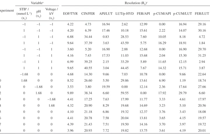
Resolutions were calculated for all pairs of compounds that coeluted at any of the sets of experimental conditions of the central composite design. So, a total of eight responses were obtained: electroosmotic flow/tyrosol (EOF/TYR); cinnamic acid/ferrulic acid (CIN/FER); apigenin/luteolin (API/LUT); luteolin/p-hydroxybenzoic acid (LUT/p-HYD); ferrulic acid/apigenin (FER/API); p-coumaric acid/apigenin (p-CUM/API); p-coumaric acid/luteolin (p-CUM/LUT); and ferrulic acid/luteolin (FER/LUT). Table 1 summarizes all the resolution response results.
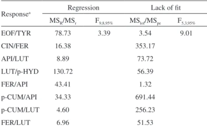
Linear and quadratic models were determined for each one of the eight responses, and each model was validated by ANOVA at the 95% confidence level. Table 2 contains the ANOVA results for the models using RS.
Table 1. Central composite design experiments and their respective resolution (RS) responses
Experiment
Variablea Resolution (R
S)c STBb /
(mmol L-1) (x1)
pH (x2)
Voltage / kV (x3)
EOF/TYR CIN/FER API/LUT LUT/p-HYD FER/API p-CUM/API p-CUM/LUT FER/LUT
1 –1 –1 –1 4.22 4.73 16.94 2.62 12.99 0.00 16.94 29.16
2 1 –1 –1 4.20 6.39 17.46 10.18 15.61 2.22 14.07 30.16
3 –1 1 –1 6.88 34.44 0.83 28.53 7.60 10.05 8.18 4.72
4 1 1 –1 9.64 37.39 3.63 43.59 5.75 16.29 18.91 1.84
5 –1 –1 1 3.60 5.20 16.90 2.88 12.68 0.00 16.90 29.70
6 1 –1 1 4.16 7.43 17.53 11.03 15.68 2.04 15.30 31.25
7 –1 1 1 6.99 39.25 2.15 33.29 5.89 11.65 12.15 2.94
8 1 1 1 9.65 40.55 3.04 44.45 7.67 14.32 15.71 3.87
9 –1.68 0 0 4.68 14.30 9.66 7.03 10.78 0.00 9.66 22.64
10 1.68 0 0 8.52 26.60 5.50 29.86 13.61 6.90 1.19 18.74
11 0 –1.68 0 3.53 3.80 19.59 0.00 12.14 2.36 17.64 27.66
12 0 1.68 0 9.89 38.34 6.60 59.55 0.00 17.92 29.79 6.60
13 0 0 –1.68 4.41 17.25 7.63 17.99 11.77 3.33 4.61 17.97
14 0 0 1.68 4.32 20.90 8.29 19.68 14.69 3.23 5.10 20.56
15 0 0 0 4.10 21.18 6.86 19.32 12.37 3.76 3.43 18.08
16 0 0 0 4.41 20.78 7.58 20.04 13.81 3.65 4.15 19.57
17 0 0 0 4.39 21.43 7.51 19.50 14.16 3.70 3.97 19.72
18 0 0 0 3.96 20.93 7.72 19.82 13.75 3.61 4.19 20.01
aCodified values of experimental factors: x
They show that almost all the models present significant lack of fit, because the MQlof/MQpe values are higher than the
critical F-value (9.01), except for the EOF/TYR (3.54) and FER/API (1.32) pairs. In this case, only these two models of the eight can be used for reliable predictions, even though all models presented significant regression results (MQR/MQr values higher than the critical F-value = 3.39).
The inability of describing the RS values with simple
models might be related to the fact that several peak crossovers occurred, altering the migration peak order. Breitkreitz et al.3 verified the same problem when the
HPLC elution order of their pesticide compounds changed.
Validation of the models built with effective mobility (µef)
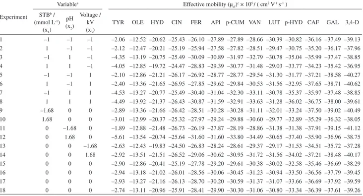
Since resolution was incapable of generating models that accurately reproduced the experimental results, the alternative was to employ the effective mobility (µef)
in model construction. In this case, the total number of responses rises to thirteen since µef is calculated for each
individual peak. The new responses were designated as TYR (tyrosol); OLE (oleuropein glycoside); HYD (hydroxytyrosol); CIN (cinnamic acid); FER (ferrulic acid); API (apigenin); p-CUM (p-coumaric acid); VAN (vanillic acid); LUT (luteolin); p-HYD (p-hydroxybenzoic acid); CAF (caffeic acid); GAL (gallic acid); and 3,4-D (3,4-dihydroxybenzoic acid). Although the number of responses for µef is almost double those for RS, one might
anticipate that the effective mobilities will have simpler
behaviors than RS upon changes in the experimental
conditions because the µef responses describe individual
peak behaviors rather than those of peak pairs. Table 3 summarizes the effective mobilities calculated for the 13 phenolic compounds.
After calculating the µef values, the mathematical
models were constructed and validated. The ANOVA results are presented in Table 4.
All the models showed significant regression results and none suffered from significant lack of fit at the 95% level, a vast improvement over the results with the resolution values.
Optimization using Derringer-Suich and resolution responses
Almost all the models for peak-pair resolutions presented lack of fit. So, these models cannot be recommended for prediction purposes. In spite of this, they were used with the desirability function to search for conditions capable of separating the phenolic compounds. The best set of conditions (STB = 1.68; pH = 0.48; V = 1.68) showed a desirability value of 0.44. As can be seen in Table 5, the predicted and the observed values differed significantly. This was expected since most the resolution models do not accurately fit the experimental results.
In Figure 1, the electropherogram resulting at this set of experimental conditions is shown. Note that luteolin (6) and apigenin (7) co-elute, presenting an experimental resolution of just 0.15, much lower than the predicted one (5.56). Furthermore the migration of all 13 compounds takes almost 50 min to occur. This long runtime is not suitable for capillary electrophoresis since it is considered to be a fast separation technique, at least when compared to HPLC, for example. These results showed that the use of models with high lacks of fit, together with multi-response optimization methods, does not lead to optimized separation conditions for the 13 compounds.
Optimization using effective mobility and interactive computer method
Optimization of multiple peak pair separation using established methods often requires a well-defined target electropherogram. Target values for resolution are relatively easy to define since they describe separations of peak pairs and permit the application of multicriteria optimization techniques employing targets. It is difficult to characterize the target using compound effective mobility values since interest centers on determining the conditions optimizing overall peak separation. Fortunately, the definition of a
Table 2. ANOVA summary considering regression statistical significance and lack of fit for linear and quadratic models with resolution (RS) as response
Responsea Regression Lack of fit MSR/MSr F9,8,95% MSlof/MSpe F5,3,95%
EOF/TYR 78.73 3.39 3.54 9.01
CIN/FER 16.38 353.17
API/LUT 8.89 73.72
LUT/p-HYD 130.72 56.39
FER/API 43.41 1.32
p-CUM/API 34.33 691.44
p-CUM/LUT 4.60 256.23
FER/LUT 6.96 51.53
Table 3. Central composite design experiments and their effective mobility (µef) responses
Experiment
Variablea Effective mobility (µ
ef)c × 105 / ( cm2 V-1 s-1 ) STBb /
(mmol L-1) (x1)
pH (x2)
Voltage / kV (x3)
TYR OLE HYD CIN FER API p-CUM VAN LUT p-HYD CAF GAL 3,4-D
1 –1 –1 –1 –2.06 –12.52 –20.62 –25.43 –26.10 –27.89 –27.89 –28.66 –30.39 –30.82 –36.16 –37.49 –39.13 2 1 –1 –1 –2.12 –12.47 –20.21 –25.19 –25.94 –27.58 –27.82 –28.51 –29.47 –30.75 –35.20 –36.17 –37.96 3 –1 1 –1 –4.35 –13.19 –20.75 –25.49 –30.09 –30.89 –31.97 –32.79 –30.78 –35.04 –35.99 –37.47 –38.85 4 1 1 –1 –4.05 –12.85 –19.72 –24.47 –28.83 –29.39 –30.77 –31.48 –29.03 –33.77 –34.23 –35.42 –36.95 5 –1 –1 1 –2.10 –12.86 –21.21 –26.17 –26.92 –28.77 –28.77 –29.54 –31.30 –31.77 –37.21 –38.58 –40.27 6 1 –1 1 –2.40 –13.36 –21.65 –26.95 –27.85 –29.62 –29.84 –30.53 –31.56 –32.95 –37.65 –38.71 –40.62 7 –1 1 1 –4.53 –13.27 –20.77 –25.49 –30.40 –31.04 –32.30 –33.11 –30.78 –35.37 –35.97 –37.48 –38.85 8 1 1 1 –4.49 –13.92 –21.37 –26.43 –30.87 –31.59 –32.91 –33.63 –31.28 –36.02 –36.75 –38.00 –39.61 9 –1.68 0 0 –2.89 –13.36 –21.66 –26.42 –28.51 –30.28 –30.28 –31.11 –32.01 –33.24 –37.50 –39.02 –40.49 10 1.68 0 0 –3.01 –12.99 –20.37 –25.32 –27.97 –29.24 –29.88 –30.60 –29.77 –32.89 –35.29 –36.32 –38.05 11 0 –1.68 0 –1.89 –12.88 –21.48 –26.73 –26.19 –27.87 –28.19 –28.86 –31.38 –31.38 –37.91 –39.15 –41.12 12 0 1.68 0 –5.61 –13.54 –20.74 –25.64 –31.60 –31.60 –33.80 –34.49 –30.65 –37.40 –35.90 –36.96 –38.75 13 0 0 –1.68 –2.63 –12.43 –19.83 –24.50 –26.83 –28.24 –28.61 –29.37 –29.17 –31.53 –34.51 –35.72 –37.28 14 0 0 1.68 –2.92 –13.51 –21.51 –26.52 –29.06 –30.62 –30.95 –31.72 –31.56 –34.02 –37.21 –38.48 –40.17 15 0 0 0 –2.90 –12.86 –20.41 –25.19 –27.78 –29.20 –29.61 –30.38 –30.02 –32.58 –35.46 –36.69 –38.29 16 0 0 0 –2.94 –13.18 –21.02 –26.01 –28.56 –30.06 –30.45 –31.23 –30.94 –33.50 –36.56 –37.79 –39.45 17 0 0 0 –2.93 –13.27 –21.16 –26.13 –28.70 –30.20 –30.59 –31.37 –31.07 –33.66 –36.69 –37.92 –39.59 18 0 0 0 –2.74 –13.11 –20.96 –25.91 –28.41 –29.90 –30.30 –31.06 –30.80 –33.34 –36.39 –37.61 –39.26
aCodified values of experimental factors: x
1 = ([STB] – 35)/10; x2 = (pH – 9.1)/0.3; x3 = (V – 26)/2; bSTB: sodium tetraborate concentration; cresponses: TYR: tyrosol; OLE: oleuropein glycoside; HYD: hydroxytyrosol; CIN: cinnamic acid; FER: ferulic acid; API: apigenin; p-CUM: p-coumaric acid; VAN: vanillic acid; LUT: luteolin; p-HYD: p-hydroxybenzoic acid; CAF: caffeic acid; GAL: gallic acid; 3,4-D: 3,4-dihydroxybenzoic acid.
Table 4. ANOVA summary considering the statistical significance of regression and lack of fit for quadratic models, employing the effective mobility (µef) as a response
Responsea Regression Lack of fit MQR/MQr F9,8,95% MQlof/MQpe F5,3,95%
µef
TYR 279.87 3.39 0.76 9.01
OLE 14.25 1.72
HYD 9.87 1.31
CIN 9.07 1.23
FER 68.65 1.33
API 38.11 0.39
p-CUM 59.23 0.17
VAN 60.33 0.16
LUT 11.36 1.23
p-HYD 55.12 0.17
CAF 11.74 1.30
GAL 13.39 1.31
3,4-D 12.23 1.38
MSR: mean square of regression; MSr: mean square of residual; MSlof: mean square lack of fit; MSpe: mean square pure error. Results reported for linear or quadratic models with smallest lack of fit values. aTYR:tyrosol; OLE: oleuropein glycoside; HYD: hydroxytyrosol; CIN: cinnamic acid; FER: ferulic acid; API: apigenin; p-CUM: p-coumaric acid; VAN: vanillic acid; LUT: luteolin; p-HYD: p-hydroxybenzoic acid; CAF: caffeic acid; GAL: gallic acid; 3,4-D: 3,4-dihydroxybenzoic acid.
Table 5. Predicted and observed (n = 3) values for the best Deringer-Suich theoretical condition (STB = 1.68; pH = 0.48; V = 1.68).
Responsea Resolution (RS) Predicted Observed
EOF/TYR 10.31 7.67 ± 0.19
CIN/FER 32.90 37.49 ± 0.40
API/LUT 5.56 0.15 ± 0.05
LUT/p-HYD 37.11 40.35 ± 0.49
FER/API 12.50 11.28 ± 0.22
p-CUM/API 9.89 11.06 ± 0.29
p-CUM/LUT 11.58 9.73 ± 0.22
FER/LUT 13.61 10.20 ± 0.22
aEOF/TYR: electroosmotic flow/tyrosol; CIN/FER: cinnamic acid/ferulic acid; API/LUT: apigenin/luteolin; LUT/p-HYD: luteolin/p-hydroxybenzoic acid; FER/API: ferulic acid/apigenin; p-CUM/API: p-coumaric acid/apigenin; p-CUM/LUT: p-coumaric acid/luteolin; FER/LUT: ferulic acid/luteolin.
target electropherogram in this application is not necessary if interactive computer graphic programs are used.
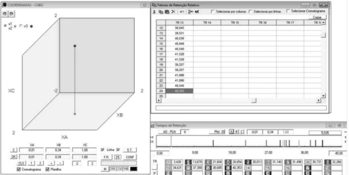
computer software and then, using only mouse or cursor movements, it was possible to search for the best separation conditions by observing the positions of all the 13 peaks that were displayed on a horizontal graphical display. As the cursor position is changed within the experimental domain defining the factor level combinations, the line positions change, simulating the electropherogram. The three most promising conditions were then tested performing validation experiments with the capillary electrophoresis system. Figure 2 illustrates a print of the software screen for the first theoretical condition.
Upon observing these three electropherograms, the first condition promotes the best separation among the peaks, and can be seen in Figure 3. The optimized condition showed a little co-elution between the apigenin (7) and luteolin (6) peaks, however, the overall separation is better than that obtained with the resolution models, and the runtime was reduced to 35 min. The model values of the effective mobilities predict that these two compounds correspond to the closest peak pair in the electropherogram. However, the model predicts that luteolin elutes slightly before apigenin, contrary to experimental observation. This discrepancy can probably be ascribed to the luteolin model. Although it does not suffer from lack of fit at the 95% confidence level its F-test value in Table 5 (1.23) is larger than the one for apigenin (0.39). Also, its predictions for the three experimental conditions in Table 6 are not as accurate.
One possible future improvement to our software would be the addition of variable peak widths to the vertical lines corresponding to each peak, since sometimes it seems that the peaks are well separated in the software, but in the experiment some peak broadening occurs and the real separations are not as good. However, this can be avoided by comparing simulated and real electropherograms for the central composite design experiments. Furthermore, one can see the simultaneous positions of all the peaks and understand their behavior when varying experimental conditions in a very didactic way.
Finally, the above results also show the robustness of the models reported here for this set of 13 phenolic
Figure 1. Electropherogram obtained for the optimum condition predicted using the models for resolution response and Derringer-Suich desirability function. Fused-silica capillary of 50 µm i.d. × 72 cm effective length with extended light path, 51.8 mmol L–1 of sodium tetraborate electrolyte, pH 9.24, 30 kV, 25 ºC, injection of 50 mbar for 5 s and detection at 210 nm. Peak identification: (0) electroosmotic flow; (1) tyrosol; (2) oleuropein glycoside; (3) hydroxytyrosol; (4) cinnamic acid; (5) ferulic acid; (6) luteolin; (7) apigenin; (8) p-coumaric acid; (9) vanillic acid; (10) p-hydroxybenzoic acid; (11) caffeic acid; (12) gallic acid; and (13) 3,4-dihydroxybenzoic acid.
compounds. Owing to operational factors, the verification experiments for the resolution models were executed almost 2 years after the design experiments, while the verification experiments for the effective mobility models were realized 3 years later (1 year between the two sets of verification experiments.) Of course for each set of verification experiments, center points of the central composite design were performed to verify reproducibility since different reagents and materials were used and laboratory infrastructure had also changed.
Conclusions
Working with single peak response values, like effective mobilities, rather than two peak functions, for example resolution, provides an attractive alternative for optimization studies. Besides determining the optimal experimental settings for peak separation, the researcher can visually see the effects on individual peak positions owing to changes in simulated experimental conditions. Peak positions that are highly sensitive to changes in specific factor levels can be studied more closely. As a result, the experimentalist will obtain a better understanding of the overall behavior of peak positions as a function of factor levels and how these levels can be manipulated to achieve the desired results. This is much easier to do than examining graphs of individual response or desirability values as a function of the factor levels as often done in current investigations. Certainly improvements can be made in our programs to more completely simulate electropherograms, such as using peak shapes of variable half-widths instead of vertical lines. Also a search engine could be included in the program to help minimize work in finding optimal conditions. These refinements are to be made in future applications so, the program will be more user-friendly to interested members of the chemical community. Finally, interactive graphical approaches of this type may be useful in multi-criteria decision making aplications in general outside the field of separation science.
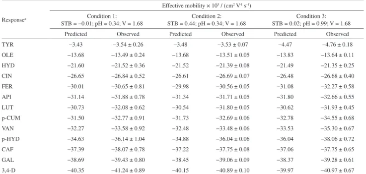
Table 6. Predicted and observed (n = 3) values for the three best conditions determined in the interactive computer method
Responsea
Effective mobility × 105 / (cm2 V-1 s-1)
Condition 1:
STB = −0.01; pH = 0.34; V = 1.68
Condition 2: STB = 0.44; pH = 0.34; V = 1.68
Condition 3: STB = 0.02; pH = 0.99; V = 1.68
Predicted Observed Predicted Observed Predicted Observed
TYR −3.43 −3.54 ± 0.26 −3.48 −3.53 ± 0.07 −4.47 −4.76 ± 0.18
OLE −13.68 −13.49 ± 0.24 −13.68 −13.51 ± 0.05 −13.83 −13.64 ± 0.11
HYD −21.60 −21.52 ± 0.36 −21.52 −21.39 ± 0.08 −21.49 −21.35 ± 0.25
CIN −26.65 −26.84 ± 0.52 −26.61 −26.69 ± 0.07 −26.48 −26.68 ± 0.40
FER −30.01 −30.65 ± 0.81 −29.98 −30.56 ± 0.05 −31.08 −32.27 ± 0.58
API −31.14 −31.88 ± 0.78 −31.34 −31.71 ± 0.05 −31.80 −32.66 ± 0.55
LUT −30.73 −32.08 ± 0.62 −30.54 −31.80 ± 0.05 −30.62 −31.93 ± 0.45
p-CUM −31.50 −32.77 ± 0.91 −31.73 −32.69 ± 0.06 −32.78 −34.55 ± 0.68
VAN −32.27 −33.58 ± 0.92 −32.48 −33.48 ± 0.06 −33.53 −35.30 ± 0.67
p-HYD −34.63 −36.14 ± 1.04 −34.88 −36.04 ± 0.06 −36.04 −38.06 ± 0.72
CAF −37.39 −38.07 ± 0.78 −37.22 −37.75 ± 0.08 −37.06 −37.75 ± 0.65
GAL −38.69 −39.43 ± 0.80 −38.45 −39.06 ± 0.09 −38.37 −39.28 ± 0.61
3,4-D −40.35 −41.24 ± 0.89 −40.15 −40.89 ± 0.10 −39.97 −40.97 ± 0.67 aTYR: tyrosol; OLE: oleuropein glycoside; HYD: hydroxytyrosol; CIN: cinnamic acid; FER: ferulic acid; API: apigenin; p-CUM: p-coumaric acid; VAN: vanillic acid; LUT: luteolin; p-HYD: p-hydroxybenzoic acid; CAF: caffeic acid; GAL: gallic acid; 3,4-D: 3,4-dihydroxybenzoic acid.
Acknowledgments
This study was carried out with the support of FAPESP (Fundação de Amparo à Pesquisa do Estado de São Paulo), Process Nr. 2008/57548-0, CAPES (Coordenação de Aperfeiçoamento de Pessoal de Nível Superior) and CNPq (Conselho Nacional de Desenvolvimento Científico e Tecnológico).
References
1. Ferreira, S. L. C.; Bruns, R. E.; Silva, E. G. P.; Santos, W. N. L.; Quintella, C. M.; David, J. M.; Andrade, J. B.; Breitkreitz, M. C.; Jardim, I. C. S. F.; Neto, B. B.; J. Chromatogr., A2000, 892, 75.
2. Siouffi, A. M.; Phan-Tan-Lou, R.; J. Chromatogr., A2000, 892, 75.
3. Breitkreitz, M. C.; Jardim, I. C. S. F.; Bruns, R. E.; J. Chromatogr., A2009, 1216, 1439.
4. Ballus, C. A.; Meinhart, A. D.; Bruns, R. E.; Godoy, H. T.; Talanta2011, 83, 1181.
5. Derringer, G.; Suich, R.; J. Qual. Technol.1980, 12, 214. 6. Kim, K. J.; Lin, D. K. J.; Appl. Statist.2000, 49, 311. 7. Khuri, A.I.; Conlon, M.; Technometrics1981, 23, 363. 8. Vining, G. G.; J. Qual. Technol.1998, 30, 309. 9. Costa, N. R.; Pereira, Z. L.; J. Chemom.2010, 24, 333. 10. Jimidar, M.; Bourguignon, B.; Massart, D. L.; J. Chromatogr., A
1996, 740, 109.
11. Gotti, R.; Furlanetto, S.; Andrisano, V.; Cavrini, V.; Pinzauti, S.; J. Chromatogr., A2000, 875, 411.
12. Loukas, Y. L.; Sabbah, S.; Scriba, G. K. E.; J. Chromatogr., A
2001, 931, 141.
13. Orlandini, I., Giannini, I.; Pinzauti, S.; Furlanetto, S.; Talanta
2008, 74, 570.
14. Hefnawy, M. M.; Sultan, M. A.; Al-Johar, H. I.; Kassem, M. G.; Aboiulenein, H. Y.; Drug Test Anal. 2012, 4, 39.
15. Fukuji, T. S.; Tonin, F. G.; Tavares, M. F. M.; J. Pharm. Biomed. Anal.2010, 51, 430.
16. Rodriguez-Méndez, M.L.; Apetrei, C.; de Saja, J. A.; Electrochim. Acta2008, 53, 5867.
17. Inarejos-Garcia, A. M.; Androulaki, A.; Salvador, M. D.; Fregapane, G.; Tsimidou, M. Z.; Food Res. Int.2009, 42, 279. 18. Bruns, R. E.; Scarminio, I. S.; Barros Neto, B., Statistical
Design - Chemometrics; Elsevier, Amsterdam, Netherlands,
2006.
19. Carrasco-Pancorbo, A.; Cruces-Blanco, C.; Segura-Carretero, A.; Fernandez-Gutierrez, A.; J. Agric. Food Chem.2004, 52, 6687. 20. G ô m e z - C a r ava c a , A . M . ; C a r r a s c o - Pa n c o r b o , A . ;
Cañabate-Diaz, B.; Segura-Carretero, A.; Fernandez-Gutierrez, A.; Electrophoresis 2005, 26, 3538.
21. Bendini, A.; Bonoli, M.; Cerretani, L.; Biguzzi, B.; Lercker, G.; Gallina-Toschi, T.; J. Chromatogr., A2003, 985, 425. 22. Bonoli, M.; Montanucci, M.; Gallina-Toschi, T.; Lercker, G.;
J. Chromatogr., A2003, 1011, 163.
23. Bonoli, M.; Bendini, A.; Cerretani, L.; Biguzzi, B.; Lercker, G.; Gallina-Toschi, T.; J. Agric. Food Chem.2004, 52, 7026. 24. Priego-Capote, F.; Ruiz-Jiménez, J.; de Castro, M. D. L.;
J. Chromatogr., A2004, 1045, 239.
25. Wang, S. P.; Huang, K. J.; J. Chromatogr., A2004, 1032, 273. 26. Carrasco-Pancorbo, A.; Gômez-Caravaca, A. M.; Cerretani, L.; Bendini, A.; Segura-Carretero, A.; Fernandez-Gutierrez, A.; J. Agric. Food Chem.2006, 54, 7984.
27. C a r r a s c o - Pa n c o r b o , A . ; G ô m e z - C a r ava c a , A . M . ; Segura-Carretero, A.; Cerretani, L.; Bendini, A.; Fernandez-Gutierrez, A.; J. Sci. Food Agric.2009, 89, 2144.
Submitted: May 10, 2013
Published online: September 6, 2013