Article
J. Braz. Chem. Soc., Vol. 24, No. 11, 1781-1788, 2013. Printed in Brazil - ©2013 Sociedade Brasileira de Química
0103 - 5053 $6.00+0.00
A
*e-mail: [email protected], [email protected]
QSAR Models of Reaction Rate Constants of Alkenes with Ozone and
Hydroxyl Radical
Yueyu Xu,a Xinliang Yu*,a and Shihua Zhang*,a,b
aCollege of Chemistry and Chemical Engineering, bNetwork Information Center,
Hunan Institute of Engineering, Xiangtan, Hunan 411104, China
As constantes de velocidade da reação do ozônio com 95 alcenos (-logkO3) e do radical
hidroxila (•OH) com 98 alcenos (-logkOH) na atmosfera foram previstas por modelos de relações
quantitativas entre estrutura e atividade (QSAR). Cálculos usando a teoria do funcional da densidade (DFT) foram realizados para os respectivos alcenos no estado fundamental e para as estruturas do estado de transição para o processo de degradação na atmosfera. Técnicas de regressão linear múltipla (MLR) e de redes neurais de regressão generalizada (GRNN) foram utilizadas para desenvolver os modelos. O modelo GRNN de -logkO3com base em três descritores e propagação ideal σ de 0,09 tem erro quadrático médio (rms) de 0,344; o modelo GRNN de -logkOH com quatro descritores e propagação ideal σ de 0,14 produz um erro rms de 0,097. Comparado com os modelos da literatura, os modelos GRNN neste artigo mostram estatísticas melhores. A importância dos descritores associados aos estados de transição na previsão de kO3e kOHnos processos de degradação atmosférica foi demonstrada.
The reaction rate constants of ozone with 95 alkenes (−logkO3) and the hydroxyl radical (•OH)
with 98 alkenes (−logkOH) in the atmosphere were predicted by quantitative structure-activity
relationship (QSAR) models. Density functional theory (DFT) calculations were carried out on respective ground-state alkenes and transition-state structures of degradation processes in the atmosphere. Stepwise multiple linear regression (MLR) and general regression neural network (GRNN) techniques were used to develop the models. The GRNN model of −logkO3 based on three
descriptors and the optimal spread σ of 0.09 has the mean root mean square (rms) error of 0.344; the GRNN model of −logkOH having four descriptors and the optimal spread σ of 0.14 produces
the mean rms error of 0.097. Compared with literature models, the GRNN models in this article show better statistical characteristics. The importance of transition state descriptors in predicting
kO3 and kOH of atmospheric degradation processes has been demonstrated.
Keywords: atmospheric degradation, general regression neural network, quantitative structure-activity relationship, reaction rate constant, transition states
Introduction
Organic compounds emitted into the atmosphere can result in many adverse effects, such as photochemical air pollution, acid deposition, long-range transport of chemicals, changes of the stratospheric ozone layer and global weather modiication, through a complex array of chemical and physical transformations.1 The reactions of
chemicals with OH radicals and ozone (O3) during the
daytime and NO3 radicals at night are the most important
degradation processes in the troposphere, so the lifetime and the upper concentration limit of the individual
chemicals is assessed by determining their reaction rate constants with •OH, •NO3 and O3. These reaction rate
constants can be obtained from experiments that may be quite costly, time-consuming, and laborious. But the experimental rate constants are available for only a limited number of organic compounds. Thus, it is useful to develop theoretical models predicting these reaction rate constants. Quantitative structure–activity relationship (QSAR) models are regression models describing the relationships between chemical structures and activities in a data-set of chemicals.2 Once a QSAR model is developed successfully,
Veber described a 6-parameter model for logkO3 of O3 and
117 organic compounds using multiple linear regression (MLR) analysis. The prediction capabilities of selected MLR model were evaluated by performing 10-fold cross-validation procedure. The average root-mean squared (rms) error in prediction of logarithm of reaction rate constants (logkO3) was 0.99.3 Gramatica et al. produced models for the estimation
of −logkO3 of O3 with 125 heterogeneous chemicals. The
optimum MLR model contained six parameters and had a
rms error of 0.73.4 Fatemi introduced a 6-parameter model
for −logkO3 of 137 organic compounds, by using artiicial neural networks (ANN). The rms errors for the training, prediction and validation sets were 0.357, 0.460 and 0.481, respectively.5 Ren et al. developed models of −logk
O3 for
116 organic compounds with projection pursuit regression (PPR) and support vector regression (SVR). The PPR model based on 7-descriptor had a rms error of 1.041 for the test set, which are smaller than the results obtained by the two SVR models (1.339 and 1.165, respectively).6 Recently,
Yu et al. used the radicals from organic compounds to calculate quantum chemical descriptors and developed 3-parameter SVR model for −logkO3. The rms errors for the training, validation and test sets were 0.680, 0.777 and 0.709, respectively.7 In addition, two MLR model of −logk
O3
in aqueous solution were, respectively, built for 39 aromatic pollutants organic compounds and 26 substituted phenols. The square regression coeficients R2 were 0.791 and 0.826,
respectively.8,9
Besides the most widely referenced AOPWIN model in EPI Suite that can be used for the calculations of reaction rate constants kOH and the accuracy of kOH was approximately 90% at 25 oC,10,11 numerous QSAR studies have also been
reported for predicting the rate constants kOH of organic compounds. Gramatica et al.reported three QSAR models for kOH with the prediction rms errors above 0.400.12,13
Öberg constructed a model with the prediction standard error of 0.501 log units, through selecting 333 descriptors and compressing to 7 latent variables.14 Böhnhardt et al.
predicted the kOH with the semiempirical AM1 method. The AM1-MOOH model yielded an overall rms error of 0.32 log units.15 Wang et al.used 22 molecular structural
descriptors to obtain a QSAR model with a rms error of 0.430 for the external validation set.16 Fatemi and Baher
developed six QSAR models of kOH for 98 alkenes with linear and nonlinear techniques. These models based on ive molecular descriptors were evaluated by a leave-24-out cross-validation test and had errors of rms≥ 0.16.17 Toropov
et al. examined the kOH of 78 organic aromatic pollutants and developed a model with correlation coeficients (r2)
for the test sets of the four random splits were 0.75, 0.91, 0.84, and 0.80.18
All these models stated above are based on descriptors from the ground states of molecules (or radicals). According to classical chemical theory, reaction rate constants correlate with the ground-state reactants and the structures of transition states (or energy-rich intermediates). These models above should be defective when only the ground-state descriptors were used. What is certainly true is that techniques for inding a transition state are more dificult than inding a ground-state structure.19 First, relatively little is known about
transition-state geometries, at least by comparison with our extensive knowledge about ground-state molecules. Second, inding a saddle point is probably (but not necessarily) more dificult than inding a minimum due to theories and techniques. Third, the energy surface in the vicinity of a transition state is likely to be more “shallow” than that of a minimum. This “shallowness” suggests that the former is likely to be less well described in terms of a simple quadratic function than the latter. Last, the transition-state calculation, in the case of radical-molecule reactions, must be carried out on open-shell system with an odd number of electrons and correlation energy must be taken into account in those calculations since it plays a vital role for the transition-state properties. Therefore, transition-state calculation is extremely hardware intensive and time-consuming. For example, transition-state optimization typically requires two to three times the number of steps as geometry optimization.19
The gas-phase reactions of the alkenes with O3 and
hydroxyl radicals are of importance as atmospheric loss processes, since the available data shows that the kO3 and
kOH values at room temperature are in the ranges of 10−15
to 10−20 and 10−10 to 10−11 cm3 molecule−1 s−1, respectively,
which are larger than the values of other compounds, such as alkanes. The purpose of this work is to produce QSAR models for kO3 of 95 alkenes and for kOH of 98 alkenes. Quantum chemical descriptors used are calculated from ground-states of reactants and energy-rich transition states of degradation processes in the atmosphere.
Methods
Statistical methods
Stepwise multiple linear regression (MLR) is used widely in seeking an optimum linear combination of variables from the subsets of the N variables.20,21 This
value for se and a high R close to 1. The t-test measures the statistical signiicance of variables. The larger (in absolute terms) a test statistic value is, the more signiicant the associated variable will be. All variables with the p-values below a speciied α cutoff values (the default level, 0.05) indicate that statistical signiicance is kept in the model.
VIF can be used to identify whether excessively high multicollinearity coeficients exist among the descriptors. Generally, descriptors with VIF < 10 show multicollinearity coeficients for descriptors do not exceed 0.90, which indicates these descriptors may be acceptable.
General regression neural network (GRNN), proposed by Specht as the category of probabilistic neural networks, is a very useful tool to perform predictions and comparisons of system performance in practice.22 Compared with other
neural networks, such as back propagation, the GRNN paradigm has the advantages that it requires no iterative training and that it is unnecessary to deine the number of hidden layers or the number of neurons per layer in advance. The basic idea of GRNN is that each (x, y) data point for an input vector to be evaluated is computed as a mean value weighted by the inluence which each Parzen window has on the input vector.22 Suppose that f(x, y) represents the known
joint continuous probability density function of a vector random variable, x, and a scalar random variable, y, and let X
be a particular measured value of the random variable x, the regression of y on X, i.e., the conditional mean, is given by:
(1)
where Ŷ is the estimate output of Y, by considering X as the system input.
The sample values Xi and Yi of the random variables
x and y can be used to estimate the density f(x, y), by introducing a nonparametric strategy based on Parzen’s window.
(2)
where n is the number of samples, p is the dimension of the vector variable x, and σ is the spreading factor (smoothing parameter or width coeficient) of Gaussian function.
By using Parzen windows estimation, the GRNN estimator can be expressed as follows:
(3)
where Di2 is a scalar function.
(4)
As the spreading factor σ becomes very large, Ŷ assumes the mean value of the observed, Yi, and as σ goes to 0, Ŷ
assumes the value of the Yi associated with the observation
closest to X. For intermediate values of σ, all values of Yi
are taken into account, but those corresponding to points closer to X are given larger weight values.22 For GRNN,
only the spreading factor σ needs to be tuned. For a bigger
σ value, the possible representation of the point of sample evaluated is possible for a wider range of X. For a small σ
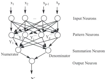
value the representation is limited to a narrow range of X. Figure 1 shows the basic structure of a GRNN including the input, pattern, summation and output layers.22 The input
layer has a full interconnection to the pattern layer and brings all of the (scaled) measurement variables X into the network. The input neurons are merely distribution units, which are equal to the dimension of the vector variable x. The pattern layer contains the Parzen windows (Gaussian activation function, exp(−Di2/2σ2), which approximates
a density function by constructing it out of many simple parametric probability density functions. The width of these Parzen windows is speciied by the spreading factor
σ. The number of units equals to the number of sample observations. The summation layer consists of two types of nodes. One belongs to the denominator nodes and the other belongs to the numerator nodes. The output unit yields the desired estimate of Ŷ values.
Data set
Supplementary Information Table S1 listed the rate constants (kO3) for the reaction of ozone with 95 alkenes,7
which were measured at 25 oC and 101.3 kPa. The
experimental data, reported in cm3 s−1 molecule−1, were
transformed to logarithmic units and multiplied by −1 to
obtain positive values. The minimum and maximum values of −logkO3 were 13.1 for α-Terpinene (No. 39) and 20.4 for 1,1-dichloroethene (No.7), respectively. The former has 10 carbon atoms and the later has 2 carbon atoms. The experimental −logkO3 values in Table S1 were randomly split into a training set (60 alkenes) and a prediction set (35 alkenes).
Supplementary Information Table S2 listed the experimental rate constants (logkOH) for the reactions of the OH radical with 98 alkenes at 25 oC and 101.3 kPa. These
experimental logkOH data have been studied by Fatemi and Baher.17 Both the training and test sets consist of 49 alkenes.
The training sets in Tables S1 and S2 were used to develop models, which were tested with respective prediction set.
Quantum chemical descriptors
The reactions between O3 and alkenes proceed by initial
O3 addition to the bond to yield an energy-rich ozonide
which rapidly decomposes to a carbonyl and an initially energy-rich biradical.1 The degradation reaction process of
alkenes with O3 can be expressed with Scheme 1.
Thus the structures of the ground-states (R1R2C1=C2R3R4)
and energy-rich transition states (R1R2C1C2(O 3)R3R4)
should correlate with the reaction rate constants (kO3). The transition-state complexes, characterized by a single imaginary vibrational frequency, were fully optimized and followed by frequency calculations. Nine quantum chemical descriptors were calculated for each transition state. These descriptors include the molecular average polarizability (αI), the molecular dipole moment (µI),
the energy of the lowest unoccupied molecular orbital (EILUMO), the energy of the highest occupied molecular orbital (EIHOMO), the most positive net atomic charge on hydrogen atoms in a molecule (qIH), the net charge of the most negative atom (qI−), the total energy(E
IT), the sum of
the Mulliken charges of O1 and O2 (Q
IO12), the sum of the
atomic polar tensor (APT) charges on C1 and C2 (q IC12).
Seven quantum chemical descriptors were derived for each ground state, which are the molecular average polarizability (αG), the molecular dipole moment (µG), the energy of the
lowest unoccupied molecular orbital (EGLUMO), the energy of the highest occupied molecular orbital (EGHOMO), the most positive net atomic charge on hydrogen atoms in a molecule (qGH), the net charge of the most negative atom (qG−), and the total energy (E
GT). All these calculations
were performed using density functional theory (DFT) in Gaussian 09 program (Revision A.02), at the B3LYP level of theory with 6-31G(d) basis set.
To fit logkOH, we calculated 12 quantum chemical descriptors from the energy-rich transition states, R1R2•C1C2(OH)R3R4, formed from the reactions of the OH
radical with alkenes (R1R2C1=C2R3R4). These descriptors
are αI, µI, EIαHOMO and EIαLUMO (for alpha spin states),
EIβHOMO and EIβLUMO (for beta spin states), qIH, qI−, E
IT, QIO12,
qIC12, and QIC12 (the sum of the APT charges on C1 and
C2 with hydrogens summed into heavy atoms). For each
ground-state alkene, the same seven descriptors (αG, µG,
EGLUMO, EGHOMO, qGH, qG−, and E
GT) were calculated. The
DFT/UB3LYP/6-31G(d) and DFT/B3LYP/6-31G(d) methods in Gaussian 09 program were respectively adopted to optimize and calculate radical transition states and ground-state alkenes.
Results and discussion
Models for reaction rate constants −logkO3
By correlating the rate constants −logkO3 of 95 organic compounds in Table S1 to the 16 descriptors calculated in this article with stepwise regression analysis,20,21 ive
MLR models (in Table 1) were obtained. In order to make a comparison with previous studies, the three parameters in Model 3 were taken as the optimal subset of descriptors, since the previous SVR model has minimum descriptors (n = 3).7 The calculation values of three parameters E
GHOMO
(the energy of the highest occupied molecular orbital of ground-state alkenes), QIO12 (the sum of the Mulliken charges on O1 and O2 of intermediates), and q
IC12 (the
sum of the atomic polar tensor (APT) charges on C1 and
C2 of intermediates) are listed in Table S1. The statistical
parameters corresponding to the standardized and
standardized regression equations based on the training set in Table S1 were summarized below:
−logkO3 = −0.562EGHOMO + 0.207 qIC12+0.319 QIO12 (5)
−logkO3 = 12.344 − 43.576EGHOMO + 0.809 qIC12
+12.188 QIO12 (6)
R = 0.926, R2 = 0.857, se = 0.558, F = 120.064, N = 60,
where R is the correlation coeficient, se is the standard error of estimation, F is the Fischer ratio, N is the number of compounds used.
The standardized coeficients in Equation 5 measure the relative importance of different variables, i.e., the larger the standardized coeficient (in absolute value) is, the more signiicant the variable will be. Usually, the non-standardized regression equations are used to predict the values of the dependent variable. The rate constants
−logkO3 calculated with Equation 6 are listed in Table S1 and depicted in Figure 2, whose error bars give a good representation of the typical 5% error in the measurement of the rate constants. The statistical results of Equation 6 are listed in Table 2. Sig.-test suggests that the three descriptors
EGHOMO, QIO12, and qIC12 are signiicant descriptors and the VIF-test shows that the descriptors are not strongly correlated with each other.
As can be seen from standardized coefficients in Equation 5 or t-test values in Table 2, the most signiicant descriptor appearing in Equation 5 is the descriptor EGHOMO, i.e., the energy of the highest occupied molecular orbital of ground-state molecules. This descriptor denotes the energetics of the reactant molecular orbitals involved in the reaction: the more reactive molecules possess a high
EHOMO.Therefore, the alkene molecule with a larger EHOMO
tends to lose electrons and leads to increased susceptibility of O3 attacking which result in a larger kO3 value. The next
two signiicant descriptor are QIO12 (the sum of the Mulliken charges of O1 and O2 of energy-rich intermediates) and q
IC12
(the sum of the atomic polar tensor charges of C1 and C2
of energy-rich intermediates), respectively. The smaller
QIO12 and qIC12 are, the larger kO3 will be. An energy-rich intermediate with the more positive net charges on C1 and
C2 or on O1 and O2 indicates that the intermediate lies in
higher energy-rich state. Thus the reaction will be relatively slow, and its kO3 will decrease.
We used the function newgrnn in MATLAB (R2012a for Windows) to build general regression neural networks (GRNN).22 The best subset of descriptors (E
GHOMO, QTO12
and qTC12) selected for the MLR models were fed to GRNN as input vectors, and the reaction rate constants −logkO3
were taken as the output. The 30-fold (or leave-two-out) cross-validation strategy was used to train GRNNs and the circulation method was used to ind the optimal spread
Table 1. Model summary for −logkO3
Model R R square Adjusted R
square
Std. error of the estimate
1a 0.873 0.763 0.760 0.672
2b 0.903 0.815 0.811 0.596
3c 0.920 0.847 0.842 0.545
4d 0.929 0.864 0.858 0.518
5e 0.933 0.871 0.864 0.506
aPredictors: (Constant), E
GHOMO; bpredictors: (Constant), EGHOMO, QIO12; cpredictors: (Constant), E
GHOMO, QIO12, qIC12; dpredictors: (Constant), EGHOMO,
QIO12, qIC12, EGLUMO; epredictors: (Constant), EGHOMO, QIO12, qIC12, EGLUMO, αI.
Table 2. Descriptor coeficients in MLR models of −logkO3
Descriptor Unstandardized coeficients Std. error Standardized coeficients t Sig. VIF
Constant 12.344 2.581 / 4.783 1.297 × 10⁻⁵ /
EGHOMO −43.576 5.751 −0.562 −7.577 3.858 × 10⁻¹⁰ 2.155
QIC12 0.809 0.220 0.207 3.686 5.164 × 10⁻⁴ 1.236
QIO12 12.188 2.712 0.319 4.495 3.545 × 10⁻⁵ 1.975
parameter σ, which varied from 0.01 to 2 with the step being 0.01. The mean square error (MSE) was used to evaluate the accuracy of GRNN models. In the end, the optimal spread
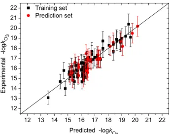
σ is determined as 0.09 and the minimum MSE value of two validation samples is 0.0041. The results from the optimal GRNN method are listed in Table S1 and depicted in Figure 3, which indicate that the predicted −logkO3 values are close to the experimental values. The rms errors of the training and test sets are 0.265 and 0.448, respectively, and the mean rms error of 95 chemicals is 0.344. These results are smaller than the corresponding values (0.540, 0.540 and 0.540, respectively) obtained from the MLR model, i.e., Equation 6. Thus the GRNN model has better prediction accuracy than the MLR model, although the latter is accurate and acceptable when compared to the previous models.3-7
We further predicted rate constants −logkO3 for the test set in Table S1 with the approaches reported by Yu et al.7 The MLR and SVR models from the training
set in Table S1 produced rms errors of 0.681 and 0.663, respectively, which are larger than that (rms = 0.448) of the present GRNN model (σ = 0.09). Therefore, combining the quantum chemical descriptors from the ground-states
and the energy-rich intermediates to predict −logkO3 of alkenes is feasible.
Models for reaction rate constants −logkOH
Similar analysis methods were used to develop QSAR models for −logkOH of 98 alkenes in Table S2. The optimal standardized and non-standardized regression equations were, respectively,
−logkOH = − 0.254µI− 0.183 EIβHOMO− 0.551 EGHOMO
+0.556 QIC12 (7)
−logkOH = 5.219 − 0.215µI− 4.284 EIβHOMO
− 16.187 EGHOMO +1.253 QIC12 (8)
R = 0.940, R2 = 0.884, se = 0.153, F = 83.692, N = 49.
The MLR model (i.e., Equation 8) of −logkOH includes a subset of descriptors: the molecular dipole moment of energy-rich intermediates (µI), the energy of the lowest unoccupied molecular orbital for alpha spin states of intermediates (EIαLUMO), the sum of the APT charges on C1 and C2 with
hydrogens summed into heavy atomsof intermediates(QIC12), and the energy of the highest occupied molecular orbital of ground-state alkenes (EGHOMO). Table 3 shows the descriptors in the MRL model all are signiicant descriptors and do not contaminate each other. As stated above, the descriptors
EIβHOMO, EGHOMO, and QIC12 are correlated with the reaction rate constants. In addition, the dipole moment descriptor µ
can relect the polarity of a molecule. A larger descriptor µI
indicates a higher reactivity, which leads to a high kOH value. The values of four descriptors and predicted −logkOH
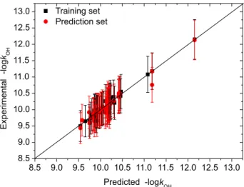
were listed in Table S2 and depicted in Figure 4 (for the MLR model) and Figure 5 (for the GRNN model). For the GRNN model with the optimal spread σ of 0.14, the rms
errors of the training and test sets are 0.069 and 0.119, respectively, which are smaller than the corresponding rms
values (0.144 and 0.134, respectively) of the MLR model (i.e., Equation 8) in this article. The mean rms errors of the MLR and GRNN models are 0.140 and 0.097, respectively. These rms errors are lower than the results (0.16-0.28)
Figure 3. Predicted vs. experimental −logkO3 values from the GRNN model for −logkO3. Error bars represent the typical 5% error in the measurement of the rate constants.
Table 3. Descriptor coeficients in MLR model of −logkOH
Descriptor Unstandardized
coeficients Std. error
Standardized
coeficients t Sig. VIF
Constant 5.219 0.394 / 13.257 5.718 × 10⁻¹⁷ /
µI −0.215 0.057 −0.254 −3.762 4.955 × 10⁻⁴ 1.728
EI HOMO −4.284 2.057 −0.183 −2.083 4.311 × 10⁻² 2.928
EGHOMO −16.187 2.116 −0.551 −7.650 1.290 × 10⁻⁹ 1.968
of the six QSAR models in the literature.17 Moreover,
compared to the literature models,17 our models have fewer
descriptors (4:5) and use more samples for the test set. We also predicted rate constants −logkOH for the test set in Table S2 with the Atkinson scheme.11,15,23,24 The rms
error of the test set is 0.210, which are larger than the results of 0.134 from the present MLR model and 0.119 from the present GRNN model (σ = 0.14). Therefore, both the MLR and GRNN models of −logkOH based on quantum chemical descriptors from ground states of reactants and radical transition states are successful in predicting −logkOH
values of alkenes.
Conclusions
QSAR models based on the MLR and GRNN approaches were successfully developed for reaction rate
constants −logkO3 of 95 alkenes and −logkOH of 98 alkenes. Quantum chemical descriptors used were obtained from the ground-states of alkenes and energy-rich transition states of degradation processes in the atmosphere. The present work tests that transition states have important effects on
kO3 and kOH of alkenes in degradation processes. Our models overcome the defects of the existing models only based on ground-state descriptors. The optimal GRNN models in this investigation are expected to have good predictive performance.
Supplementary Information
Tables S1 and S2 showing experimental rate constants and descriptors used are available free of charge at http:// jbcs.sbq.org.br as PDF ile.
Acknowledgements
The study was supported by the Natural Science Research Foundation of Hunan Province (No. 12JJ6011) and the National Natural Science Foundation of China (Grant No. 20972045).
References
1. Atkinson, R.; Atmos. Environ. 2007, 41, 200.
2. Karelson, M.; Lobanov, V. S.; Katritzky, A. R.; Chem. Rev. 1996, 96, 1027.
3. Pompe, M.; Veber, M.; Atmos. Environ. 2001, 35, 3781. 4. Gramatica, P.; Pilutti, P.; Papa, E.; QSAR Comb. Sci. 2003, 22,
364.
5. Fatemi, M. H.; Anal. Chim. Acta 2006, 556, 355.
6. Ren, Y.; Liu, H.; Yao, X.; Liu, M.; Anal. Chim. Acta 2007, 589, 150. 7. Yu, X.; Yi, B.; Wang, X.; Chen, J.; Atmos. Environ. 2012, 51,
124.
8. Jiang, J.; Yue, X.; Chen, Q.; Gao, Z.; Bull. Environ. Contam. Toxicol. 2010, 85, 568.
9. Liu, H.; Tan, J.; Yu, H.; Liu, H.; Wang, L.; Wang, Z.; Int. J. Environ. Res. 2010, 4, 507.
10. Atkinson, R.; Chem. Rev. 1986, 86, 69.
11. Kwok, E. S. C.; Atkinson, R.; Atmos. Environ. 1995, 29, 1685. 12. Gramatica, P.; Pilutti, P.; Papa, E.; Atmos. Environ. 2004, 38,
6167.
13. Gramatica, P.; Pilutti, P.; Papa, E.; J. Chem. Inf. Comput. Sci. 2004, 44, 1794.
14. Öberg, T.; Atmos. Environ. 2005, 39, 2189.
15. Böhnhardt, A.; Kühne, R.; Ebert, R.-U.; Schüürmann, G.;
J. Phys. Chem. A 2008, 112, 11391.
16. Wang, Y.; Chen, J.; Li, X.; Wang, B.; Cai, X.; Huang, L.; Atmos.
Environ, 2009, 43, 1131. Figure 4. Predicted vs. experimental −logkOH values from the MLR model
for −logkOH. Error bars represent the typical 5% error in the measurement of the rate constants.
17. Fatemi, M. H.; Baher, E.; SAR QSAR Environ. Res. 2009, 20, 77.
18. Toropov, A. A.; Toropova, A. P.; Rasulev, B. F.; Benfenati, E.; Gini, G.; Leszczynska, D.; Leszczynski, J.; J. Comput. Chem. 2012, 33, 1902.
19. Hehre, W. J.; A Guide to Molecular Mechanics and Quantum Chemical Calculations, Wavefunction Inc.: California, 2003. 20. Fatemi, M. H.; Baher, E.; Ghorbanzade'h, M.; J. Sep. Sci.2009,
32, 4133.
21. Yu, X.; Yi, B.; Wang, X.; J. Comput. Chem. 2007, 28, 2336. 22. Specht, D. F.; IEEE Trans. Neural Networks 1991, 2, 568. 23. Atkinson, R; Chem. Rev. 1985, 85, 69.
24. Atkinson, R.; Int. J. Chem. Kinet. 1987, 19, 799.
Supplementary Information
Printed in Brazil - ©2013 Sociedade Brasileira de Química0103 - 5053 $6.00+0.00S
I
*e-mail: [email protected], [email protected]
QSAR Models of Reaction Rate Constants of Alkenes with Ozone and
Hydroxyl Radical
Yueyu Xu,a Xinliang Yu*,a and Shihua Zhang*,a,b
aCollege of Chemistry and Chemical Engineering, bNetwork Information Center,
Hunan Institute of Engineering, Xiangtan, Hunan 411104, China
Table S1. Quantum chemical descriptors and -logkO3 values for 95 alkenesa
No. Name EGHOMO / a.u. qIC12 / a.u. QIO12 / a.u. -logkO3 (exp.) -logkO3 (pred.)b -logkO3 (pred.)c Training set
1 1,3-Cyclohexadiene -0.205526 0.687946 -0.608815 14.7 14.44 14.93
2 Bicyclo(2.2.1)-2-heptene -0.230909 0.539394 -0.603226 14.7 15.49 14.86
3 1,3-Cycloheptadiene -0.208367 0.726131 -0.599350 15.8 14.71 15.55
4 Carvomenthene -0.230995 0.712092 -0.565545 15.3 16.09 15.82
5 Terpinolene -0.215923 0.683347 -0.615165 14 14.81 14.06
6 Tetrafluoroethene -0.254209 2.531489 -0.530281 19 19.01 19.00 7 1,1-dichloroethene -0.266297 1.353019 -0.453706 20.4 19.51 20.31 8 2-methyl-1-butene -0.239266 0.688732 -0.553380 16.8 16.58 16.48 9 Hexafluoropropene -0.281063 1.928487 -0.532637 19.1 19.66 19.10 10 2-(chloromethyl)-3-chloro-1-propene -0.277909 0.622758 -0.539928 18.4 18.38 18.40 11 1.2-Propadiene -0.262966 0.788560 -0.561417 18.72 17.60 18.72 12 1-Methyl-1-cyclopentene -0.223285 0.689486 -0.590023 15.17 15.44 15.40 13 2-Methyl-1.4-pentadiene -0.241725 0.684857 -0.537600 16.89 16.88 16.94 14 1.2-Dimethylcyclohexene -0.216046 0.690035 -0.591053 15.68 15.11 15.44 15 Trans-3-Hexene -0.235597 0.681452 -0.556782 15.77 16.38 16.09 16 3-methyl-1-butene -0.249284 0.692447 -0.530566 16.96 17.30 16.99 17 Trans-2,5-Dimethyl-3-hexene -0.235390 0.658580 -0.566235 16.39 16.23 16.06 18 Cis- +trans-3,4-Dimethyl-3-hexene -0.215528 0.709946 -0.592469 15.42 15.09 15.44 19 Cis-Cyclooctene -0.231456 0.726928 -0.558084 15.43 16.22 15.87
20 Propene -0.249793 0.721658 -0.524060 16.9 17.43 16.95
21 Cis-2-Butene -0.233323 0.762977 -0.561473 15.8 16.29 15.91
22 1-Pentene -0.246525 0.709157 -0.531907 17 17.18 16.98
No. Name EGHOMO / a.u. qIC12 / a.u. QIO12 / a.u. -logkO3 (exp.) -logkO3 (pred.) b -logk
O3 (pred.) c
Training set
38 Cis-Ocimene -0.219579 0.719544 -0.528799 14.7 16.05 15.04 39 α-Terpinene -0.192386 0.696624 -0.636419 13.1 13.54 13.10 40 1,1-Difluoroethene -0.262252 1.613112 -0.527680 18.7 18.65 18.70 41 Cis-1,3-dichloropropene -0.266567 0.951379 -0.479781 18.8 18.88 18.79 42 Acrolein -0.257123 0.558858 -0.487809 18.3 18.06 18.30 43 Methyl vinyl ketone -0.247851 0.547462 -0.558508 17.4 16.78 17.39 44 2-cyclohexen-1-one -0.236331 0.578369 -0.519273 17.7 16.78 17.69 45 3.3-Dimethyl-1-butene -0.249533 0.662849 -0.539712 17.28 17.18 17.10 46 Cis-5-Decene -0.231212 0.722127 -0.563115 15.92 16.14 15.84 47 Cis-3-Hexene -0.231830 0.710888 -0.561279 15.82 16.18 15.86
48 Ethene -0.266547 0.702671 -0.504672 17.7 18.38 17.70
49 2.3-Dimethyl-1.3-butadiene -0.224837 0.690641 -0.548631 16.58 16.01 16.29 50 2-methyl-1,3-butadiene -0.226117 0.696111 -0.525793 16.89 16.35 16.24 51 Cis-2,trans-4-Hexadiene -0.208020 0.773115 -0.549613 15.5 15.34 15.67 52 Cycloheptene -0.230329 0.701853 -0.562377 15.5 16.10 15.82 53 1,4-Cyclohexadiene -0.226180 0.653269 -0.611527 16.2 15.28 16.08 54 Bicyclo(2.2.2)-2-octene -0.234554 0.703257 -0.600302 16.1 15.82 16.03 55 1,3,5-Cycloheptatriene -0.212641 0.746006 -0.544032 16.3 15.58 16.07 56 d-Limonene -0.225634 0.715009 -0.574389 15.2 15.75 15.56 57 Trifluoroethene -0.254416 2.080157 -0.533009 18.9 18.62 18.90 58 Methacrolein -0.255129 0.558435 -0.517032 18 17.61 17.97 59 Vinyl chloride -0.262460 1.064558 -0.470593 18.6 18.91 18.61 60 Cis-1,2-dichloroethene -0.259607 1.323410 -0.446518 19.2 19.29 19.29
Test set
61 Trichloroethene -0.261331 1.615179 -0.431117 19.5 19.79 19.33 62 Octafluoro-2-butene -0.303156 1.409374 -0.534576 20.2 20.18 19.10 63 Cyclopentene -0.232844 0.693015 -0.564597 15.56 16.17 15.89 64 2.3-Dimethyl-2-butene -0.217788 0.749722 -0.580553 14.82 15.37 15.43 65 2-Ethylbutene -0.238800 0.682848 -0.553128 16.89 16.56 16.44 66 2.4-Dimethyl-1.3-butadiene -0.215685 0.795419 -0.538723 16.1 15.82 15.91 67 Trans-4-Octene -0.234244 0.696825 -0.560270 15.85 16.29 15.97 68 3-methyl-1-pentene -0.248993 0.699206 -0.535291 17.31 17.24 17.03 69 Trans-2,2-Dimethyl-3-hexene -0.235538 0.651240 -0.601851 16.38 15.80 15.89 70 1,3,5-Hexatriene -0.209225 0.751076 -0.536485 16.6 15.53 16.02 71 2-Methyl-2-propene -0.239539 0.717789 -0.545965 16.9 16.71 16.71 72 Trans-2-Butene -0.235027 0.740022 -0.550173 15.6 16.48 16.12 73 cis-2-Pentene -0.232569 0.723065 -0.543939 15.7 16.43 16.00 74 2-Methyl-2-butene -0.225635 0.748689 -0.578196 15.4 15.74 15.51 75 4-Methyl-1-pentene -0.249099 0.705650 -0.522110 17 17.41 16.95 76 Cis-3-Methyl-2-pentene -0.224347 0.734981 -0.566204 15.3 15.81 15.67 77 1-Heptene -0.246201 0.707874 -0.532087 16.9 17.16 16.98 78 α-Pinene -0.218341 0.770965 -0.591064 15.7 15.28 15.39 79 D3-Carene -0.224523 1.025169 -0.532474 15.9 16.47 16.33 80 γ-Terpinene -0.217922 0.685046 -0.580884 15.6 15.32 15.44 81 3-methyl-2-isopropyl-1-butene -0.237362 0.622156 -0.560336 17.48 16.36 16.20 82 4-Methyl-1-cyclohexene -0.233595 0.688425 -0.555796 16.09 16.31 15.96 83 2.3.3.-Trimethylbutene -0.239373 0.647121 -0.559572 17.08 16.48 16.37 84 1-Butene -0.246661 0.707276 -0.521192 16.9 17.31 16.94
85 1-Decene -0.246066 0.712919 -0.522230 17 17.28 16.94
86 Myrcene -0.222559 0.699391 -0.530152 14.9 16.15 15.53
87 Vinyl fluoride -0.260366 1.174156 -0.532133 18.2 18.15 18.70 88 Trans-1,2-dichloroethene -0.259885 1.295515 -0.474002 18.7 18.94 19.10
Table S1. continuation
No. Name EGHOMO / a.u. qIC12 / a.u. QIO12 / a.u. -logkO3 (exp.) -logkO3 (pred.) b -logk
O3 (pred.) c
Test set
89 Cis-1,2-difluoroethene -0.254139 1.645013 -0.523658 18.6 18.37 18.70 90 Trans-1,3-dichloropropene -0.262766 1.039316 -0.457231 18.2 19.06 18.60 91 2.3-Dimethyl-1-butene -0.239239 0.669720 -0.558808 16.89 16.50 16.37 92 3-penten-2-one -0.240713 0.554961 -0.538358 16.7 16.72 16.94 93 Cis-4-Octene -0.233860 0.714750 -0.546147 16.02 16.46 16.06 94 Trans-2,trans-4-Hexadiene -0.207551 0.781737 -0.562995 15.4 15.16 15.59 95 Cyclohexene -0.233459 0.706416 -0.545016 15.9 16.45 16.04
aExperimental data taken from: Yu, X.; Yi, B.; Wang, X.; Chen, J.; Atmos. Environ. 2012, 51, 124; b-logk
O3 values predicted from the MLR model for
-logkO3; c-logk
O3 values predicted from the GRNN model for -logkO3.
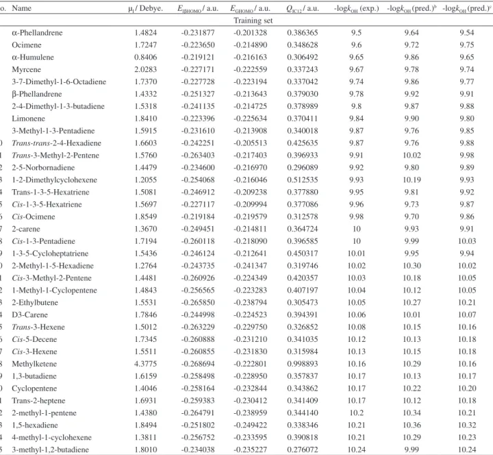
Table S2. Quantum chemical descriptors and -logkOH values for 98 alkenes a
No. Name µI / Debye. EIβHOMO / a.u. EGHOMO / a.u. QIC12 / a.u. -logkOH (exp.) -logkOH (pred.) b -logk
OH (pred.) c
Training set
No. Name µI / Debye. EIβHOMO / a.u. EGHOMO / a.u. QIC12 / a.u. -logkOH (exp.) -logkOH (pred.) b -logk
OH (pred.) c
Training set
36 α-pinene 1.7989 -0.254171 -0.218341 0.393235 10.26 9.95 10.11 37 Cis-2-butene 1.7860 -0.262610 -0.233323 0.408649 10.26 10.25 10.21 38 Camphene 1.4010 -0.263749 -0.233314 0.272334 10.27 10.17 10.19 39 2,3-dimethyl-1-butene 1.6013 -0.266191 -0.239239 0.314830 10.28 10.28 10.21 40 2,3,3-trimethylbutene 1.6417 -0.263018 -0.239358 0.328902 10.3 10.28 10.23 41 Cis-Cyclooctene 1.6066 -0.253752 -0.231830 0.347259 10.38 10.15 10.22 42 Bicycle(2, 2, 2)-2-Octene 1.4061 -0.255391 -0.234580 0.460586 10.39 10.38 10.30 43 4-methyl-1-pentene 1.5886 -0.262981 -0.249101 0.338715 10.42 10.46 10.46 44 1-Decene 1.8493 -0.258003 -0.246066 0.335645 10.43 10.33 10.42 45 1-Butene 1.8309 -0.259331 -0.246661 0.324568 10.5 10.34 10.43 46 3,3-Dimethyl-1-Butene 1.5682 -0.263495 -0.249531 0.304249 10.55 10.43 10.47 47 Cis-1,3-Dichloroperopene 3.2949 -0.294107 -0.266567 0.944536 11.08 11.27 11.08 48 1-Chloroethene 1.9759 -0.279475 -0.262491 0.632896 11.18 11.03 11.18 49 Cis-1,2-Difluoroethene 1.8755 -0.314502 -0.254139 1.325095 12.15 11.94 12.15
Test set
50 α-Terpinene 2.0858 -0.232670 -0.192386 0.435730 9.44 9.43 9.54 51 Trans-Ocimene 1.7246 -0.223649 -0.214890 0.348622 9.6 9.72 9.75 52 Terpinolene 1.3946 -0.228190 -0.215923 0.490789 9.65 10.01 9.86 53 1-3-5-Hexatriene 1.5081 -0.246912 -0.209238 0.377880 9.66 9.81 9.92 54 2-5-Dimethyl-2-4-Hexadiene 1.9270 -0.235355 -0.194584 0.439269 9.68 9.51 9.58 55 γ-Terpinene 1.7112 -0.232884 -0.217922 0.401595 9.75 9.88 9.81 56 1-3-Cyclohexadiene 2.2179 -0.243968 -0.205526 0.411646 9.79 9.63 9.88 57 Cis-2-trans-4-Hexadiene 1.3842 -0.238352 -0.207100 0.424245 9.81 9.83 9.85 58 1-3-Cycloheptadiene 1.6743 -0.233355 -0.216948 0.337400 9.86 9.79 9.84 59 4-Methyl-1-3-Pentadiene 1.6156 -0.233286 -0.207910 0.359410 9.88 9.69 9.84 60 2-3-Dimethyl-1-3-Butadiene 1.8076 -0.248685 -0.224837 0.372377 9.91 10.00 10.11 61 β-Caryophyllene 1.2463 -0.221001 -0.219970 0.304256 9.92 9.84 9.74 62 2-5-Dimethyl-1-5-Hexadiene 1.8965 -0.238133 -0.233258 0.350638 9.92 10.05 10.21 63 Trans-1-3-Hexadiene 1.8150 -0.264811 -0.215871 0.359915 9.95 9.91 10.00 64 2-3-Dimethyl-2-Butene 1.4108 -0.259953 -0.217816 0.516044 9.96 10.20 9.96 65 Dimethylketene 4.7987 -0.261749 -0.211921 1.031781 9.97 10.03 10.16 66 2-Methyl-1-3-Butadiene 1.3600 -0.258270 -0.226117 0.348285 10 10.13 10.12 67 1-4-Cyclohexadiene 1.5143 -0.236744 -0.226180 0.330141 10 9.98 9.90 68 Trans-1-3-Pentadiene 1.5856 -0.263320 -0.216601 0.311442 10 9.90 9.97 69 2-3-Dimethyl-2-Pentene 1.5624 -0.258862 -0.211185 0.464335 10.01 9.99 9.94 70 1-Methylcyclohexene 1.2382 -0.254919 -0.224366 0.418505 10.03 10.20 10.05 71 2-Methyl-2-Pentene 1.5670 -0.263738 -0.221978 0.403204 10.04 10.11 10.01 72 Trans-1-4-Hexadiene 1.8623 -0.240840 -0.230689 0.343403 10.04 10.01 10.15 73 2-Methyl-2-Butene 1.7199 -0.255803 -0.225635 0.412442 10.06 10.11 10.12 74 2-Heptene 1.6930 -0.259383 -0.230412 0.341406 10.07 10.12 10.18 75 2-Methyl-1-4-Pentadiene 1.3669 -0.243179 -0.239354 0.339253 10.1 10.27 10.04 76 Cycloheptene 1.4482 -0.256849 -0.232142 0.381290 10.13 10.24 10.21 77 Cis-4-octene 1.3845 -0.261839 -0.231550 0.312938 10.14 10.18 10.17 78 Trans-4-octene 1.6524 -0.258211 -0.229560 0.398424 10.16 10.18 10.18 79 Cyclohexene 1.7324 -0.255118 -0.233459 0.329525 10.17 10.13 10.22 80 Trans-2-pentene 1.4261 -0.262505 -0.230681 0.334536 10.17 10.19 10.16 81 Cis-2-pentene 1.6360 -0.259237 -0.232569 0.396460 10.18 10.24 10.21 82 Trans-2-butene 1.6587 -0.260163 -0.235027 0.361226 10.22 10.23 10.21 83 2-methyl-1-butene 1.4756 -0.265263 -0.239266 0.333624 10.22 10.33 10.21 84 Trans-4-methyl-2-pentene 1.4187 -0.259956 -0.235456 0.378799 10.22 10.31 10.21 85 Sabinene 1.9228 -0.254161 -0.221302 0.396345 10.25 9.97 10.14 86 2-methyl-1-propene 1.5207 -0.265485 -0.239567 0.359728 10.26 10.36 10.22
No. Name µI / Debye. EIβHOMO / a.u. EGHOMO / a.u. QIC12 / a.u. -logkOH (exp.) -logkOH (pred.) b -logk
OH (pred.) c
Test set
87 Trans-4,4-dimethyl-2-pentene 1.5498 -0.260832 -0.232897 0.293190 10.26 10.14 10.18 88 1,4-Pentadiene 1.7022 -0.252850 -0.240502 0.307939 10.27 10.21 10.31 89 Bicycle(2, 2, 1)-2-heptene 1.5115 -0.258902 -0.230925 0.305581 10.31 10.12 10.18 90 Longifolene 1.5343 -0.258575 -0.229710 0.287896 10.35 10.08 10.17 91 1-Heptene 1.8080 -0.261668 -0.246201 0.315476 10.39 10.33 10.43 92 1-Octene 1.5705 -0.262658 -0.246141 0.326022 10.4 10.40 10.41 93 1-Hexene 1.8387 -0.258431 -0.246307 0.335618 10.43 10.34 10.42 94 3-methyl-1-Butene 1.7204 -0.260006 -0.249824 0.309133 10.49 10.39 10.45 95 1-Pentene 1.8387 -0.258858 -0.246525 0.335080 10.5 10.34 10.42 96 Ketene 2.5412 -0.303842 -0.240468 0.703868 10.76 10.75 11.18 97 1-Bromoethene 1.8529 -0.276904 -0.254441 0.577348 11.17 10.85 11.18 98 Trans-1,2-Difluoroethene 1.4297 -0.322054 -0.253777 1.301103 12.13 12.03 12.15
aExperimental data taken from: Fatemi, M. H.; Baher, E.; SAR QSAR Environ. Res. 2009, 20, 77; b-logk
OH values predicted from the MLR model for -logkOH; c-logk
OH values predicted from the GRNN model for -logkOH.