BIOLOGICAL AND OCEANOGRAPHIC UPWELLlNG INDICATORS AT CABO FRIO (RJ)

Rev. bras. oceanogr., 45(1/2):11-23, 1997

BIOLOGICAL AND OCEANOGRAPHIC UPWELLlNG INDICATORS AT

CABO FRIO

(RJ)

Gleyci A. O. Moser & Sônia M. F. Gianesella-Galvão

Instituto Oceanográfico da Universidade de São Paulo (Caixa Postal 66 I49, 05315-970 São Paulo, SP, Brasil)

.

Abstract: Phytoplankton biomass, chemical parameters and hydrology were studied in a

transect 101.6 km long offCabo ]<'rio(RJ), Southeast Brazil, during summer (December 29 to 31, 1991) and winter (June 27 to 30, 1992). Wind induced upwelling events are frequently observed in the area during summer, becoming rare during winter. By the summer cruise a bloom of phytoplankton was observed in surface, close to the coast, with chlorophyll concentrations reaching 25.55 mg Chl-a m.3, uncoupled from the cold, nutrient rich waters of South Atlantic Central Water (SACW), found below 40 m depth. During the winter cruise, the SACW raised at the surface waters in front of Cabo Frio depicting an upwelling event. However, in spite of high surface nitrate concentrations (up to 7.7 11M)ch10rophyll-a were lower than 2 mg Chl-a m'3. The phytop1ankton biomass, meteorological and hydro10gical data suggest a probable upwelling event immediately before the summer cruise, and an ongoing one during winter time. Cluster analyses and principal component ana1yses(PCA) were applied to summer and winter data, pointing out multidimensional fronts in the area during both seasons.

.

Resumo: A biomassa fitoplanctônica, parâmetros químicos e hidrologia foram

estudadas em um transecto de 101,6 Km ao largo de Cabo Frio, (RJ) Brasil, durante o verão (Dezembro 29 a 31, 1991) e inverno (Junho 27 a 30, 1992). Nesta área, eventos de ressurgência induzidos pelo vento são comuns durante o verão, tomando-se mais raros durante o inverno. Durante o período de verão uma floração de fitoplâncton foi observada na superficie próximo ao continente, apresentando um máximo de clorofila-a igual a 25,55 mg Cl-a m,3 desacoplado das águas frias e ricas em nutrientes da Água Central do Atlântico Sul (ACAS), presente abaixo de 40 m. Durante o inverno, a ACAS alcançou a superficie em frente a Cabo Frio, caracterizando um evento de ressurgência. Entretanto, apesar das altas concentrações de nitrato na superficie (até 7,7 11M),as concentrações de clorofila-a foram menores do que 2 mg Cl-a m'3. Os dados meteorológicos, hidrológicos e de biomassa fitoplanctônica sugerem um provável evento de ressurgência imediatamente anterior ao período de amostragem de verão e um evento em andamento durante o inverno. Análises de agrupamento e de componentes principais (ACP) foram aplicadas às coletas de verão e inverno separadamente, mostrando frentes multidimensionais na área, durante as duas estações.

.

Descriptors: Ch10rophyll, Water Masses, Upwelling, Spatial Distribution, Cabo Frio,

Brazil.

.

Descritores:Clorofila, Massas de Água, Ressurgência, Distribuição Espacial, Cabo Frio,

Brasil.

12 _{Rev. bras. oceanogr.. 45(1/2). 1997}

Introduction

The Cabo Frio region is a meeting point fot

three water masses: Continental Water (CW) and Tropical Water (TW- Brazil Current) at surface, and the South Atlantic Central Water (SACW) at bottom (Aidar et ai., 1993; Valentin, et al., 1987). Under

NNE winds surface water moves towards off shore, due to Coriolis action resulting in the upwelling of SACW. This situation changes when southern cold fronts reach the area (Valentin op. cit., 1987). The

prevailing surface water masses in thifcase are CW and TW.

Gonzalez-Rodriguez et ai. (1992) identified

three different phases for the upwelling phenomenon at Cabo Frio: the "upwelling phase", when cold, nutrient rich water reaches the surface; the "productive phase", characterized by high

phytoplankton biomass and low nutrient

concentration; and the "downwelling phase" characterized by decreasing phytoplankton biomass and nutrient concentration.

This work presents the spatial distribution of phytoplankton biomass related to the oceanographic structure at Cabo Frio. The sampling points are grouped by their ecological similarities determined by multivariate analyses aiming to identify the geographical distribution of these upwelling evolution indicators during the summer and winter of 1992.

23020

Material and method

Samplings were carried out at 9 oceanographic stations along a transect off Cabo Frio (22°00' S, 42°00' W to 22°40' S, 41°00' W, RJ, Brazil) during summer (December 29 to 31, 1991) and winter (June 27 to 30, 1992). Data on wind intensity and velocity were obtained at a meteorological station in Arraial do Cabo (RJ) by the Instituto de Estudos do Mar Almirante Paulo Moreira. For summer survey the wind data were recorded at 12 h intervals and at 3 h intervals during the winter.

At each station, samples were taken at O, 5, 10, 20, 50, 100 and 150 m according to local depth (Fig. 1). Temperature and salinity were obtained by Cacciari et ai. (1994), using aCTD (SeaBird modo

SeaCat, cod. 808) and water was collected with Van Dom bottles for nitrate, nitrite, phosphate, silicate, organic and inorganic suspended matter, chlorophyll and phaeophytin. Samples for suspended matter and pigment analyses were retained under filtration over GF/F Whatman@ filters. All samples were kept in dark at -20°C until the laboratory analyses. Transparency was also estimated, using a Secchi disk.

o 13250 26500 397505300066250 79500

I I I I f I I

Scale (m)

Fig. 1. Study area and oceanographic station sites.

42°00'W 41°00'W

+

+

Atlantic Ocean

+

,,5

+

+

."1

MOSER & GlANESELLA-GALVÃO: Upwelling indicators at Cabo Frio 13

Thermohaline intervals for the water masses identification were defined according to Miranda & Katsuragawa (1991) to SACW and TW, and according to Aidar et ai. (1993) to CW. The

considered thermohaline intervals applied to thl;se water masses as well as the intervals for the mixtures among them are presented in Table 1,. Euphotic zone (Zeu) was calculated from the relation Zeu=2.8*S, where S is the Secchi Disc reading (Aidar et ai., op. cit.). Mixing zone inferior boundary (Zm) was here

defined as the thermocline topo

Table I. Thennohaline intervals defined to the water masses present at Cabo Frio area, according to Aidaret aI.(1993) and Miranda & Katsuragawa (1991)

Analyses of nitrate and nitrite were carried out according to Aminot & Chaussepied, (1983), dissolved phosphate and silicate according to Grasshoff et ai. (1983), organic (OSM) and

inorganic (ISM) suspended matter as described in APHA (1965), and chlorophyll-a and phaeophytin following Lorenzen (1967).

Principal component analyses (PCA) and cluster analyses, combining the Ward method and square Eudidean distance (Legendre & Legendre, 1983) were applied to the data (FITOPAC software, Shepard, 1994) aiming to look up the main distribution tendency and to provide statistical support to the condusions. The power of PCA lies in the ability to identif)r the most efficient basis for representing the data and thereby to determine the dominant pattems of spatial and temporal variability (Mariano et ai., 1996). Initially a PCA was applied

to the entire data set. This analysis pointed out the main differences between these seasons. To a better understanding of data distribution tendencies, PCA and duster analyses were applied to summer and winter surveys apart.

Results

Summer

The available wind data set for summer showed little consistence to determine the prevailing winds

before the sampling arising (Fig. 2a, b), in account of the low sampling frequency. Water temperature was higher at the layers above 40 m (maximum 24.7°C), decreasing sharply below this depth reaching values lower than 13°C at 120 m (Fig. 3a). Surface salinity values were below 36 at coastal stations and above this value at off shore stations (beyond 40 km). From 40 m down to the battom salinity values were below 36 (Fig. 3b). According to the thermohaline intervals (Table 1), CW was found at the surface (above 10 m) dose to the coast (Fig. 3c) while TW was found at the surface about 40 km off shore, but an intrusion of TW was observed inshore under CW (stations 1, 2 and 3). SACW was present in the layers below 40 m along the entire transect. The Zm depth was around 25 m at stations 1 and 2. From station 3 up to station 8, the mean Zm depth was around 50 m and at station 9 it reached 150 m. The Zeuwas equal to or deeper than Zmexcept for station 3 where Zmwas 10 m deeper than Zeu (Fig. 4 ).

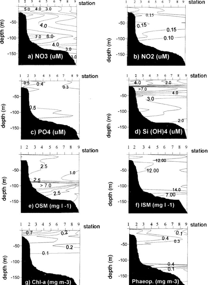
Nitrate concentrations were below 0.5 flM in surface waters, increasing to 7 flM toward the shelf bottom (Fig. 5a). Nitrite concentrations were below 0.05 flM at surface water and above 0.10 flM dose to battom at the off shore stations, but at stations 3 and 4, this nutrient reached 0.40 flM at 80 m (Fig. 5b). Pattems of phosphate distribution were similar to nitrate. Higher concentration values were associated with SACW (> 0.70 flM) and the lower values were

associatedwith TWand CW« 0.2flM)(Fig. Se).

Silicate concentrations showed maxima at mid water (> 6.0 flM), at the surface, dose to the shore

(stations 1 and 2, > 3.0 flM) and dose to the battom

at coastal stations (Fig. 5d). The distribution of OSM and ISM (Fig. 5e and 5i) followed a similar pattem, with high concentrations within CW and at mid depths but with lower concentrations dose to the battom.

Chlorophyll-a reached an extremely high value at the surface of stations 2 (25.55 rng Chl-a m,3) and 3 (13.06 mg m'3). Except for these maxirna, concentrations remained below 5.64 mg m,3 at the coastal stations decreasing sharply with depth (Fig. 5g). Phaeophytin distribution followed this same pattem, but the highest value was 1.2 mg m,3 at the surface ofstation 2 (Fig. 5h).

Winter

During the winter the prevailing winds carne

1TomNNE, changing to SSE two days before the

sampling arising and than reverted again to NNE with velocities around 10 m S.l one day before the beginning ofthe survey (Figs 6a and b).

Water masses PC S

SACW T < 18 S<36

SACWICW 18<T<20 35,4 < S < 36

CW T>20 S < 35,4

SACWrrw 18 < T < 20 S > 36

cwrrw T>20 35,4 < S < 36

14 _{Rev. .bras. oceanogr.. 45(1/2). 1997}

Fig. 2. Prevailing winds prior to and during the sampling period (summer). The zero in the graphs represents the samp1ing origino(A) Wind rose (x axis is the East-West component velocity (m/s), y axis is the South-North component ve10city (m/s», (B) Stick plot diagram (x axis represents time (d'ays),y axis is the vectorial wind veiocity (m/s».

a) 1 2 3

Temperature, salinity

and water masses distributionduringsummer

4 5 6 7 8 9_Stations b) 1 2 3 4 5 6 7 8 9_Stallons. c) 1 2 3 4 5 6 7 8 9 _Stations

Fig. 3. Temperature, salinity and water masses vertical distribution during summer survey.

Stations

o

o 2 3 4 5 6 7 8 9

.50

- LocalDepth -8- Zeu -8-Zm

-100

Depth -150

.200

Fig. 4: Zm and Zeu for summer.

mIs Sampling

beginning

10

5f I / ,[

+\J

/

r

\ \ /

Of

mIs 2

\

\j

o \ \ I1 /\

\1 \

r

-- 1/

\ \ 2 \ I \i

\

-5f

"

,

\,

\

i'

A

,6

B

"

-101

mIs -100- ₁₀ 13

-10 -5 o 5 10 2 5 7 _{t (days)}

:[ .111!111!!I!!!IIII'!,IIII:w.41Iill!II'llli,,1,a:lJ g .

'-

g -5_

_tm"""

..c:

.-:ttf:::::::::::::',

i

ã.

.g 7- .g -10

.. :...-...!Jh!:ni;ir:iD:r;:;:;/;::;_{...'...,......} :;.;....;.: '; : ;_.

. . . , . . '::::::':1

MOSER & GIANESELLA-GAL VÃO: Upwelling indicators at Cabo Frio 15

2 3 4 5 6 7

8 9, station 2 3 4 5 6 7 8 9 station

-

_{E -5}

'-'"

2 3 4 5 6 7 8 9

_station

3 4 5 6_I 7 8 9

station

-50

-100

-

_E

'-'

..c

Q.

Q) 'U

-150

2345678

9 station 2 3 4 5 6 7 8 9 station

2 3 4 5 6 7 8 9 station 1 2 3

1

5 6 7 8 9 station

Fig. 5. Vertical distribution of chemical and biological variables during summer (stations x depth). a) Nitrate(jlM), b) Nitrite (jlM),d) Silicate(jlM),e) OSM (mg r\ f) ISM (mg r\ g) Chlorophyll-a (rJg m-\ h) Phaeophytin (mg m-3).

-501_I

I

I

-

-100

E

'-'

..c

Q.

-150

Q)

'U

-50

-

_E

-100

'-'

..c

Q.

Q) 'U _-150

-50.

Y

-50

-

_E

-'-'" -1 00

E

-100

..c '-'

11. _..c

Q) _ã.

'U _{-150 Q) -150}

'U

-50

_-=----

_0.2

-50

-

--..s -100

_'-'"

E

-100

..c ..c

11. Q.

Q) -150

I

Q) _-150

16 _{Rev. bras. oceanogr., 45(112), 1997}

Fig. 6. Prevailing winds prior to and during the sampling period (winter). The zero in the graphs represents the sampling origino (A) Wind rose (x axis is the East-West component velocity (m/s), y axis is the South-North component velocity (m/s», (B) Stick plot diagram (x axis represents time (days), y axis is the vectorial wind velocity (m/s».

Lowtemperaturevalues« 17.5°e) were found at the entire water column in the coastal stations (Fig. 7a). Temperature was above 20°C at surface waters at stations 5 to 9. The 18°C isotherm reached surface waters near station 2, and varied from 50 m to 100 m far from the coast. Salinity (Fig. 7b) was above 36 onlyat surface waters off shore. SACW was observed at the bottom throughout the transect and reached surface waters near the continent. TW was

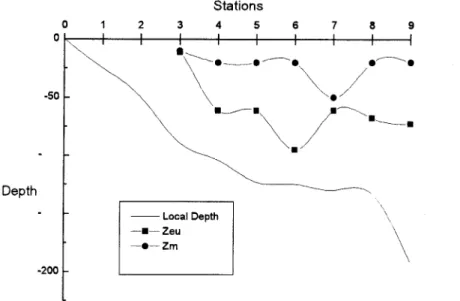
found far from the coast (40 Km) from surface down to 40 m depth. CW was not detected at that time (Fig. 7c). The z". depth (Fig. 8) was around 25 m, except at station 7 where it got down to 50 m depth and at stations 1 and 2 where the upwelled water filled the entire water colwnn. The z.,u was always deeper than the z"., reaching depths below 50 m off shore.

Temperature. Salinity and water mass distribution during winter.

Fig. 7. Temperature, salinity and water masses vertical distribution during winter survey.

mls 2O[ N

50 Sampling

40

mls 30

+

beginning

A

20

"

B

-3)1

:: /7/ "1

ri1L

-20 -10 O 10 20 mls -3_ o o 2 5 7 10 12 t(days)15

Stations Stati ons

. I, : :L.s,!.\ I I I I I

I I

Stations

L..., I I ). \ ,<

I I _"

I ₎ I I I _,.lt..,..J

a)

I

:5 c. Q) 'C

MOSER & GIANESELLA-GALVÃO: Upwelling indicators at Cabo Frio 17

o

o

2 3

Stations

4 5 6 7 8 9

.~.

8'\--0-

_\

\

y-O~

'.

~

/

~

8

~

8 8

8 -50

Depth

- LocalDepth

-8- 2eu -.-2m

-200

Fig. 8. Zm and Zeu for winter.

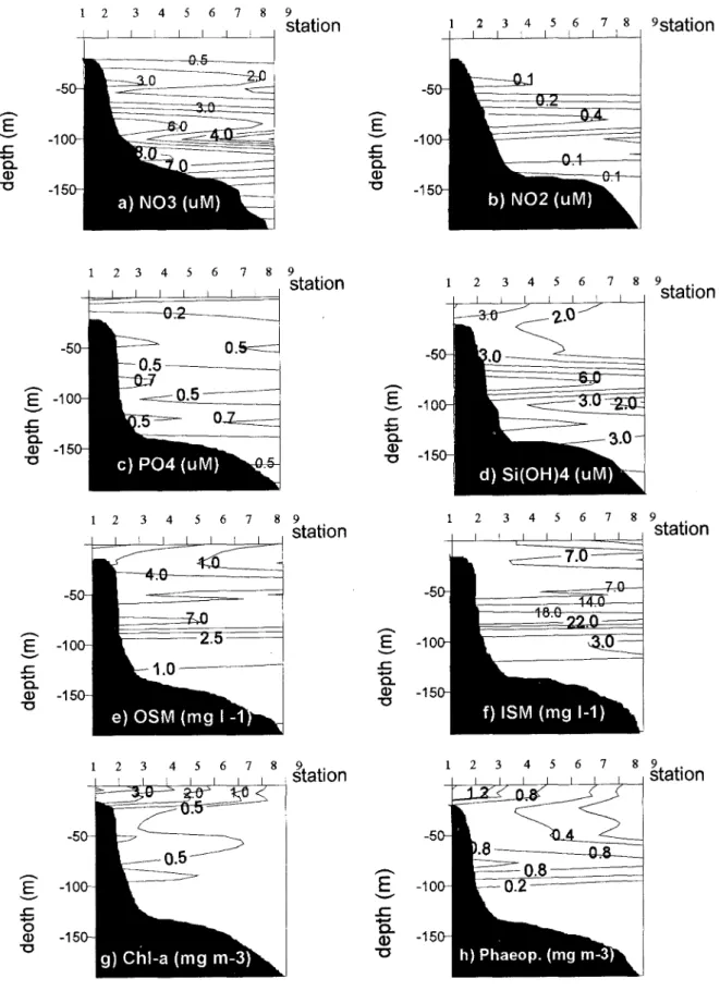
High nitrate concentrations were associated with SACW (2.8 to 7.7 /lM) (Fig. 9a). Nitrite concentrations were generally low reaching values above 0.15 !J.Mclose to the coast in surface and mid waters (Fig. 9b). Phosphate exhibited the same distribution pattem as nitrate with higher values associated to SACW (above 0.4 !J.M) (Fig. 9c). Silicate showed the highest concentrations (above 4 !J.M)at the stations 1, 2 and 3 at mid water. This nutrient was also high (~3/lM)near the shelfbottom

(Fig. 9d). OSM concentrations showed a maximum at mid water (> 7 mg rI around 100 m). The concentrations decreased down to the bottom and toward off shore. Maximum values of ISM were found close to the shelf and at mid water (> 12 mg rI around 120 m) (Fig. ge, f).

Phytoplankton biomass as chlorophyl1-a was below 1.3 mg Chl-a m'3 in coastal stations (Fig. 9g). The biomass distribution decreased with distance ITom the coast and depth increment. For off shore waters chlorophyll-a values did not reach 1 mg Chl-a m,3. Phaeophytin concentrations were low and showed a distribution similar to chlorophyll-a, with a maximum value ofO.4 mg m-3(Fig. 9h).

Statistical Treatment

The cluster analyses applied to the data parceled out three groups with ecological similarities: A, B and C, for both summer and winter. These groups were plotted spatially as classed posts (Fig. 10), showing differences between the spatial distribution of the upwelling indicators. For both seasons the sampling points were grouped in a similar way. Group A is composed by stations 1,2 and 3. During summer, the sampling points of these stations were

grouped ITom surface to 20 and 40 m depth, while during winter it included sampling points down to the bottom. Group B is represented by sampling points far ITomthe coast (stations 4 to 9) and above 50 m depth. Group C is composed by sampling points below 50 m depth. During summer this group is represented just by stations 4 to 9 while during winter deep points of stations I to 3 were part of this group as well.

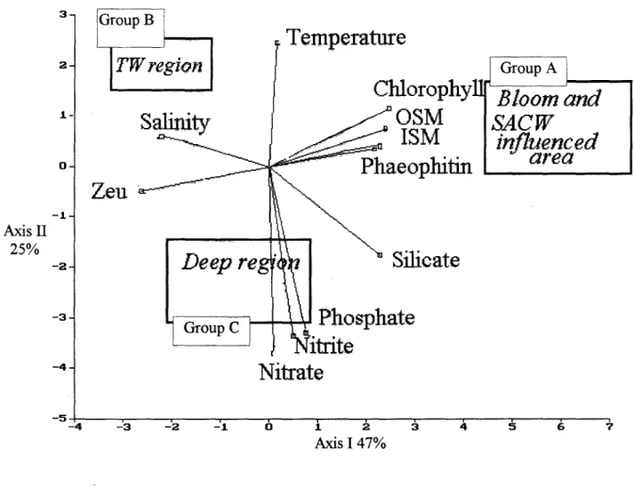
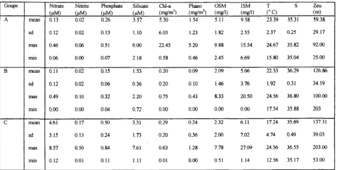
The PCA applied to summer data (Fig. 11) showed resembling results to those of cluster analysis. Axis 1 (47% of total variance) is related to chlorophyll-a, OSM, ISM, phaeophytin and silicate vectors in its positive section and to salinity and Zeu vectors in its negative section. Group A has a positive projection in axis L It is composed by sampling points with high chlorophyl1concentrations (mean value 5.30 mg Chl-a m'3) associated with low salinity (mean value 35.31) (Table 2). Group B, projected negatively in this axis, is characterized by low chlorophyll concentration (mean value 0.20 mg Chl-a m'3) and high salinity (36.29). Axis 1 is also related to chlorophyll variation due to the distance ITomthe shore and depth increment.

18 Rev. bras. oceanogr., 45(1/2), 1997

1 2 3 4 5 6 7 8 ~tation

2 3 6 7 8 9

t

t

.

S a lon

4 5

2 3 4 5 6 7 8 9station

2 3 4 5 6 7 8 9

t

t

.

S a lon

Fig. 9. Vertical distribution of chemical and biological variables during winter (stations x depth). a) Nitrate (jlM), b) Nitrite (1lM),d) Silicate (1lM),e) 08M (mg rI), f) IBM (mg ri), g) Chlorophyll-a (mg m'3), h) Phaeophytin (mg m'3).

2 3 4 5 6 7 8 9

station 1 2 3 4 5 6 7 8

9

station

-5

.-

.-E

E

-

---

--a.

a.

Q) Q)

"C "C

I

d) Si(OH)4 (uM) , !

1 2 3 4 5 6 7 8 9 1 2 3 4 5 6 7 8 9

.

station ' statlon 7.0

-50_

-

-5

.-

.-E

E

-

_-10

-

_-10

--

_a.

--

_a.

Q) Q)

"C _11': "C _-15

.-

.-E

E

-

---

--a.

a.

Q) Q)

"C "C

-.

.-

_E

E

-

--.c

--

...

o a.

Q) _Q)

MOSER & GIANESELLA-GALVÃO: Upwelling indicators at Cabo Frio 19

3

Temperature

Zeu~

Chlorophy.

~

OSM

.

ISM

~aeOPhi1in

Group A

-1---Bloomand

SACW

influenced

_area

2

_{TW regiQfl}

J.-o

-J.

Axis II

25%

-2

Silicate

-3

_Phosphate

I!l

itrite

Nitrate

-4

-5

-4 -3 -2 -J. o J. 2 3

Axis I 47%

4 5 6 7

Fig. 11. PCA applied to summer data. Groups A (+), B (O) and C (O).

o 1 3 4 7 8 9 _O 1 2 3 4 5 6 7 8 9

O O

-20 -20

-40 -40

+ -o O -o -o -o

--

+

+

<> -o O -o O

-60 -60

-80 <>

-80

"

-o

-100 <) -100 -o

<) -o

-120 -o -120 <> -o -o

-140 -140

-160 -160

-180 -180

Summer

Winter

20 _{Rev. bras. oceanogr., 45(1/2), 1997}

Table 2. Average, standard deviation, maximum and minimum value for each group individualized by cluster analysis during summer survey.

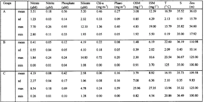
PCA (Fig. 12) performed for the winter survey also parceled out the sampling points into three groups: two under SACW influence, above and below Zeu(groups A and C) and a third group (group B) out ofSACW influence. In axis I ofPCA (51.79% oftotal variance) nitrate, nitrite, phosphate, ISM and OSM vectors were positively projected. Temperature, salinity and Zeuvectors were negatively projected in this axis. Group A was related to axis I positive section. This group is characterized by low temperatures (mean value 16.59°C) and the highest nutrient concentrations (Table 3). Group B was related to the negative section ofaxis I and showed

4l I 3J

I

I

I 21,

i I

Axis II .1

l

'

]643%

o~ I I

i

-.11

I

I -21

I

-3~ -4

Temperature

o"

Sabnity

~

TW

"'-l

'"

influencc;

area ItZeu

//

~/

Zeu

Group B

Deep

Region

high salinity and temperature (mean values 36.19 and 22.61°C, respective1y). This axis represents the hydrological condition of the area, revealing points above Zeu,under SACW or TW influence.

Chlorophyll and phaeophytin vectors are related to axis II (16.43% oftotal variance) positive section. Associated to the negative section were group C sampling points with low phytoplankton biomass (chlorophyll-a mean value 0.06 mg Chl-a m-3) and high nitrate concentration (4.19 11M). Axis II represents the biological response variation with depth.

Chlorophyll

I

Phaeophitin

{

_V

_/"

Nitrit

/

Silicate

ISM

OSM

Phosphate

Nitrate

o .1

A'dS I 5179"'0

Fig. 12. PCA applied to winter data. Groups A (+), B (O) and C (<».

-3 -2 -.1 :2 3 4 5

Goups NitIate Nitrite Phosphate Silicate CW-a Phaeo OSM ISM T S Zeu

(J.LM) (J.LM) (J.LM) (J.LM' (mg'm3) (mg'm3) (mg'l) (mg'l) (OC) (m)

A mean 0.13 0.02 0.26 3.57 5.30 1.54 5.Il 9.58 23.39 35.31 59.38

sd 0.12 0.02 0.13 1.10 6.05 1.23 1.82 2.55 2.37 0.25 29.17

max 0.46 0.06 0.51 6.00 22.45 5.20 9.88 15.54 24.67 35.82 92.00

min 0.06 0.00 0.07 2.18 0.58 0.46 2.45 6.69 15.80 35.04 25.00

B mean 0.11 0.02 0.15 1.53 0.20 0.09 2.09 5.06 22.33 36.29 126.86

sd 0.12 0.02 0.06 0.36 0.20 0.10 1.46 3.76 1.92 0.31 34.19

max 0.49 0.10 0.32 2.20 0.75 0.43 8.33 20.50 24.56 36.80 100.00

mm 0.00 0.00 0.04 0.72 0.00 000 0.00 0.00 17.54 35.88 203

C mean 4.61 0.17 0.50 3.31 0.29 0.24 2.32 6.11 17.24 35.69 137.31

sd 3.15 0.13 0.24 1.73 0.20 0.36 2.00 7.02 4.74 0.49 39.03

max 8.57 0.50 0.84 7.61 0.63 1.28 7.78 27.09 24.56 36.55 203.00

MOSER & GIANESELLA-GALVÃO: Upwelling indicators at Cabo Frio 2]

Table 3. Average, standard deviation, maximum and minimum values for each group individualized by cluster analysis during winter survey.

Discussion

Physical, chemical and biological variations at Cabo Frio continental shelf seems to be more related to local wind conditions and water masses than to seasonal cycles (André, 1990). The prevailing wind direction during the whole year in Cabo Frio comes from NNE, excepting when cold fronts reach the region, reverting the wind direction to SSW (Valentin et aI., 1987). During summer the number

of cold fronts that arrived at the Brazilian southeast coast before sarnplings were at the expected range: seven frontal systerns during December. The last one carne over Cabo Frio from 25 to 29, Dec/1991 (Climanálise, 1991), immediately before the summer survey. The shallow Zeu depth (25 m) at station 3 during this period was probably due to the back scattering and absorbency of light promoted by the high phytoplanktonic biomass since ISM showed low concentrations. Inside the euphotic zone nitrate and other nutrients were depleted, but chlorophyll-a concentrations reached its maximum (25.55 Chl-a mg m,3) and phaeophytin concentration attained only 5.2 mg m,3 pointing out a healthy phytoplankton status. According to Holligan et aI. (1984), these

conditions indicate that nutrients coming from deep layers have been actively absorbed by phytoplankton. The phytoplankton biomass exhibited extremely high concentrations when compared to the usual biomass levels observed in the area during upwelling events: 0.5-6.0 mg Chl-a m-3(Valentin et aI., 1987). Present

data were comparable to those from the Benguela upwelling, (NW-Africa) that ranges from 15 to 31

mg Chl-a m,3 (Estrada, 1980) and from Peru upwelling that ranges from 10 to 40 mg Chl-a m-3 (Strickland et aI., 1969), known as the most

productive upwelling areas.

During June of 1992 (winter), five cold frontal systems carne over Brazil (Climanálise, 1992), a number below the expected for the period (at least 7 cold frontal systems). The El Niiío South Oscillation (ENSO) occurrence during this winter strengthened the cold fronts at the brazilian south region and weakened them at the southeast sea coast. During the winter survey, as observed during summer, z... was always above 4u. However, the 18°C isotherrn was deeper during winter than during summer at off shore stations (>70 Km) and followed Zeudepth. The observed SACW advection close to the coast promoted nutrient enrichment at the euphotic zone. However, chlorophyll-a concentrations during this period « 1.3 mg Chl-a m-3)were lower than during summer.

The PCA for summer showed major variations in chlorophyll-a concentrations specially observed close to the coast. Major nutrient variations were also associated to this period. The low nitrate concentrations found at the coastal stations are probably a consequence of nitrate exhaustion by phytoplankton. According to Syret (] 981), the phytoplankton preferentially uptakes ammonia instead of nitrate or nitrite. This author observed higher nitrite values associated to high levels of chlorophyll-a in the field. High nitrite variability during summer could be related to a previous nitrate consumption and reduction to nitrite by microalgae

Goups Nitrate Nitrite Phosphate Silicate ChI-a Phaeo OSM ISM T S Zeu

IJ,1M) IJ,1M) IJ,1Mi IJ,1M) (rngm-3) (rngrn.3) (rngl.l) (rngl.t) ("C) (rn)

A rnean 5.51 0.18 0.56 5.20 OA6 0.27 3.08 12.39 16.59 35.52 36.03

sd 1.23 0.03 0.14 2.32 0.33 0.09 0.85 4.29 2.13 0.19 15.79

max 7.70 0.26 0.95 12.10 1.36 0.40 4.85 19.00 15.79 35.82 54.60

min 2.80 0.11 0.33 1.93 0.05 0.05 1.92 5.50 0.19 35.00 17.92

B mean OA1 0.05 0.12 4.19 0.22 0.08 1.48 6.19 22.60 36.19 110.98

sd 0.55 0.04 0.05 4.10 0.18 0.05 0.39 2.02 2.09 OAO 10.14

max 1.84 0.24 0.24 14.85 0.72 0.20 2.30 10.6 23.54 36.67 125.00

min 0.00 0.01 0.04 1.08 0.00 0.00 0.91 3.70 125 35.00 100.80

C mean 4.19 0.08 0.42 2.58 0.06 0.16 3.79 8.92 16.55 35.73 109.58

sd 2.27 0.04 0.17 1.06 0.08 0.16 7.08 6.36 2.10 0.35 9.83

max 8.54 0.18 0.69 4.78 0.24 0.59 25.96 27.35 13.96 35.32 125.00

22 _{Rev. bras. oceanogr., 45(1/2), 1997}

and later excretion of this nutrient. During summer, however, the high concentrations of chlorophyll-a observed in coastal stations were associated to low nitrate concentrations and to CW. These findings suggest that the SACW reached the surface layers and mixed with CW in previous periods, conducting to an enrichment of these waters and promoting phytoplankton growth. Mariano et aI. (1996)

modeling the bio-physical variability in a Gulf Stream meander crest aided by PCA, identified regions with enhanced pigment biomass, uncoupled from regions with low temperature and high nutrient concentrations. Present data suggest that summer conditions represent the productive phase as defined by Gonzalez-Rodriguez et aI, (1992) for upwelling

evolution.

Winter survey, however, was associated to high nitrate concentrations due to the strong SACW advection. The low chlorophyll-a concentration observed dose to Cabo Frio suggests that phytoplankton may be in a lag growth phase.

Saldanha (1993) observed that under low

temperatures« 18°C), similar to those from surface waters in Cabo Frio, phytoplankton takes over four days to reach its exponential growth phase. The nutrient addition to the euphotic zone occurs just prior to the phytoplankton biomass enhancement. Models from simple Lagrangian calculations applied to eddy simulations of the Gulf Stream suggested that a chlorophyll distribution partem similar to those observed at the present work can also arise from a simple meandering stream. Olson et a/.

(1994) showed that the time it takes to the phytoplankton response, moves the resultant increase in biomass downstream. The area dose to Cabo Frio presented strong winds from NNE to SSW since one day before the sampling arise. According to André (1990) wind speeds higher than 3.5 m S.l and continuously acting for at least 24 hours precede SACW advection at Cabo Frio region.

Summer and winter surveys represented different upwelling status. The conditions showed during summer survey suggest that the upwelling phenomenon was in its "productive phase", sensu

Gonzalez-Rodriguez et aI.(1992), meaning that the

physical upwelling processes had already ceased and nutrients were then part of the internal pool of the phytoplankton. However, during winter all the analyzed features suggested an initial upwelling phase considered by those authors as the physical upweIling processes properly, when cold, rich nutrient water arises at the surface and the phytoplankton had not sufficient time to incorporate the nutrients in its biomass.

The reflex of the upwelling on both surface temperature and phytoplankton biomass can be

observed down to the northem sector of the South brazilian bight (Ubatuba region), as described by Lorenzetti & Gaeta (1996). The clusters and PCAs spatial portrayals pointed out vertical and horizontal boundaries of a multidimensional environment represented by physical, chemical and biological characteristics. In both periods, these analyses allowed the spatial observation of a group of sampling points (group A) with ecological similarities inside the 100 m isobath, which represents the very inner shelf directly influenced by the upwelling action. Moser (1997) and Gianesella-Galvão (1994) analyzing data from Cabo Frio up to Rio Paraíba do Sul estuary from a survey that followed both samplings of the present paper, did not observe high phytoplankton biomass at Bacia de Campos, even after the summer bloom. This findings strengthen the idea of frequent patch displacements southward.

Acknowledgmen ts

The authors thank PETROBRÁS and CAPES for the financial support. The paper benefited from comments by Or. Ian C. Campbell (Monash University, Australia), or. Afrânio R de Mesquita (Instituto Oceanográfico, Universidade de São Paulo) and our anonymous referees.

References

Aidar, E.; Gaeta, S. A.; Gianesella-Galvão, S.M.F.; Kutner, M. B. B. & Teixeira C. 1993. Ecossistema costeiro subtropical: nutrientes dissolvidos, fitoplâncton e cIorofila-a e suas relações com as condições oceanográficas na região de Ubatuba (SP). Publção esp. Inst. oceanogr., S Paulo, (10):9-43.

Aminot, A. & Chaussepied, M. 1983. Manuel des analyses chimiques en millieu marin. Brest, C.N.EX.O. 376p.

André, D. L. 1990. Análise de parâmetros

hidroquímicos na ressurgência de Cabo Frio. Dissertação de mestrado. Universidade Federal Fluminense, Instituto de Geociências. 203p.

MOSER & GIANESELLA-GALVÃO: Upwelling indicators at Cabo Frio 23

Cacciari, P. L.; Harari, 1.; Pereira, 1. E. R. & Talaska, A, 1994. Identificação e distribuição das massas d'água e da corrente de superficie sobre a plataforma e talude continental da Bacia de Campos no verão e no inverno de 1992. In: Programa de monitoramento ambiental oceânico da Bacia de Campos (RJ). Relatório final. São Paulo, FUNDESPA p 302-372.

Climanálise. 1991. Boletim de monitoramento e análise climática. Sistemas frontais e frontogênese. Climanálise, 6( 12):22.

Climanálise. 1992. Boletim de monitoramento e análise climática. Sistemas frontais e frontogênese. Climanálise, 7(6):27.

Estrada, M. 1980. Phytoplankton biomass and production in the upwelling region of NW Africa. Relationships with hidrographic parameters. Mar. Biol., 60: 63-71.

Gianesella-Galvão, S. M. F. 1994. Nutrientes, biomassa e matéria em suspensão. In: Programa de monitoramento ambiental oceânico da Bacia de Campos (RJ). Relatório final. São Paulo, FUNDESPA p 432-445.

Gonzalez-Rodriguez, E.; Valentin, J. L., André, D. L. & Jacob, S. A 1992. Upwelling and downwelling at Cabo Frio (Brazil): Comparison of biomass and primary production responses. J. Plankt. Res., 14 (2): 289-306.

Grasshoff, F.; Ehrhardt, M. & Kremiling, K. 1983.

Methods of seawater analysis. 2nd ed.

WIENHIEN, Verlag Chemie. 419p.

Holligan, P. M.; Pingree, R. D. & Mardell, G. T. 1985. Oceanic solutions, nutrient pulses and phytoplankton growth. Nature, 314(6009):348-350.

Legendre, L. & Legendre, P. 1983. Numerical ecology. Amsterdam, Elsevier. 419p.

Lorenzen, C. J. 1967. Determination of chlorophyll and pheopigments: spectrophotometric equation. Limnol. Oceanogr.~ 12:343-346.

Lorenzetti,1. A & Gaeta, S. A 1996. The Cape Frio upwelling effect over the South Brazil Bight northern sector shelf waters: a study using AVHRR images. International Archives of Photogrammetry and Remote Sensing, 31(B7): 448-453.

Mariano, A. 1., Hitchcock, C. J. A., Ashjian, C. J., Olson, D. B., Rossby, T., Ryan, E. & Smith, S. L. 1996. Principal component analysis of biological and physical variability in a Gulf Strem meander crest. Deep-Sea Res., 43(9): 1531-1565.

Miranda, L. B. & Katsuragawa, M. 1991. Estrutura térmica na região sudeste do Brasil (outubro-novembro de 1988). Publção esp. Inst. oceanogr., S Paulo, 8:1-14.

Moser, G. A O. 1997. Estudo da distribuição da biomassa fitoplanctônica e de variáveis oceanográficas na Bacia de Campos (RJ), utilizando um sistema de informações geográficas (SIG). Dissertação de mestrado. Universidade de São Paulo, Instituto Oceanográfico. 149 p.

Olson, D. B., Hitchcok, C. J. A., Mariano, A. J., Ashjian, C. J., Peng, G., Nero, W.R. & Podestá, G. 1994. Life on the edge: marine life and fronts. Oceanology, 7: 52-60.

Saldanha, F. M. P. 1993. Simulação da mistura vertical de massas d'água da região de lJbatuba (SP), efeitos sobre a produção primária e biomassa fitoplanctônica. Dissertação de mestrado. Universidade de São Paulo, Instituto Oceanográfico. 2 v.

Shepard, G. J. 1994. FITOPAC I. Manual de usuário.

Universidade Estadual de Campinas,

Departamento de Botânica, 88 p.

Strickland, J. D. H.; Eppley, R.W. & Mendiola, B.R. 1969. Phytoplankton populations, nutrients and photosynthesis in the Peruvian coastal waters. Boln Inst. Mar Perú, 2(1):37-45.

Syret, P. J. 1981. Nitrogen metabolism of microalgae. 182-210. In: Platt, T. ed. Physiological bases of phytoplankton ecology. CanoBulI. Fish. aquat. Sei., (2\ 0):346p.

Valentin, J. L.; André, D. L. & Jacob, S.A. \987. Hydrology in the Cabo Frio (Brazil) upwelling: two-dimensional structure and variability during a wind cycle. Continent. ShelfRes., 7(1):77-88.