Modeling long-term changes of the Black Sea ecosystem characteristics

(1)

OSD

9, 2039–2080, 2012

Modeling long-term changes of the Black

Sea ecosystem characteristics

V. L. Dorofeyev et al.

Title Page

Abstract Introduction

Conclusions References

Tables Figures

◭ ◮

Back Close

Full Screen / Esc

Printer-friendly Version

Interactive Discussion

Discussion

P

a

per

|

Dis

cussion

P

a

per

|

Discussion

P

a

per

|

Discussio

n

P

a

per

Ocean Sci. Discuss., 9, 2039–2080, 2012 www.ocean-sci-discuss.net/9/2039/2012/ doi:10.5194/osd-9-2039-2012

Ocean Science Discussions

This discussion paper is/has been under review for the journal Ocean Science (OS). Please refer to the corresponding final paper in OS if available.

Modeling long-term changes of the Black

Sea ecosystem characteristics

V. L. Dorofeyev1, T. Oguz2, L. I. Sukhikh1, V. V. Knysh1, A. I. Kubryakov1, and G. K. Korotaev1

1

Marine Hydrophysical Institute National Academy of Sciences, Sevastopol, Ukraine

2

Institute of Marine Sciences Middle East Technical University, Erdemli, Turkey

Received: 28 February 2012 – Accepted: 17 April 2012 – Published: 16 May 2012

Correspondence to: V. L. Dorofeyev (dorofeyev viktor@mail.ru)

(2)

OSD

9, 2039–2080, 2012

Title Page

Tables Figures

◭ ◮

Back Close

Full Screen / Esc

Discussion

P

a

per

|

Dis

cussion

P

a

per

|

Discussion

P

a

per

|

Discussio

n

P

a

per

|

Abstract

A three dimensional coupled physical-biological model is provided for the Black Sea to investigate its long-term changes under the synergistic impacts of eutrophication, climatic changes and population outbreak of the gelatinous invaderMnemiopsis leidyi. The model circulation field is simulated using the high frequency ERA40 atmospheric

5

forcing as well as assimilation of the available hydrographic and altimeter sea level anomaly data for the 30 yr period of 1971–2001. The circulation dynamics are shown to resolve well the different temporal and spatial scales from mesoscale to sub-basin scale and from seasonal peaks to decadal scale trend-like changes. The biogeochemi-cal model includes the main vertibiogeochemi-cal biologibiogeochemi-cal and chemibiogeochemi-cal interactions and processes

10

up to the anoxic interface zone. Its food web structure is represented by two phytoplank-ton and zooplankphytoplank-ton size groups, bacterioplankphytoplank-ton, gelatinous carnivoresMnemiopsis and Aurelia, opportunistic species Noctiluca scientillans. The nitrogen cycling is ac-commodated by the particulate and dissolved organic nitrogen compartments and the dissolved inorganic nitrogen in the forms of ammonium, nitrite and nitrate. The

ecosys-15

tem model is able to simulate successfully main observed features and trends of the intense eutrophication phase (from the early 1970s to the early 1990s), but points to its modification to simulate better the ecosystem conditions of the post-eutrophication phase.

1 Introduction 20

The Black Sea is one of the largest enclosed basins in the world, which has been receiving relatively high nutrient load from rivers draining parts of Europe and Asia. The Black Sea marine ecosystem manifested significant changes since the 1960s in response to the nutrient enrichment, overfishing and large population growth of gelatinous and opportunistic species. These changes altered severely biomass,

tax-25

(3)

OSD

9, 2039–2080, 2012

Title Page

Tables Figures

◭ ◮

Back Close

Full Screen / Esc

Discussion

P

a

per

|

Dis

cussion

P

a

per

|

Discussion

P

a

per

|

Discussio

n

P

a

per

northwestern shelf. The classical phytoplankton annual cycle with spring and autumn maxima in biomass has been modified by additional blooms – the summer one being the most pronounced. These changes in the food web structure were also accom-panied by modifications in the vertical geochemical structure. The most evident ones were an increase of nitrate concentration in the nitracline zone from 2 to 3 mmol m−3in

5

the late 1960s to 6–9 mmol m−3 during the 1980s and broadening of the suboxic zone (Konovalov and Murray, 2001).

The ecosystem dynamics and its reorganisations during di_fferent phases of the ecosstem changes of the Black Sea have been studied by a series of one-dimensional coupled physical-biogeochemical models (Oguz et al., 2000, 2001, 2008; Lancelot

10

et al., 2002; Gregoire et al., 2008). Their three-dimensional extensions are provided by Gr égoire and Lacroix (2003), Gr égoire and Friedrich (2004), Gr égoire et al. (2004), Dorofeyev (2009), Korotaev et al. (2011). The present study extends these studies by employing a three-dimensional coupled physical-ecosystem model to study evolution of the ecosystem from 1971 to 2001. One particular feature of the model is the

assimila-15

tion available hydrographic and current measurements into the circulation model. The period 1971–1994 involved relatively dense hydrographic surveys and was replaced by the availability of altimetry data from the Topex/Poseidon and ERS missions after-wards. Reanalysis of the Black Sea dynamics for 1971–1993 performed by Moiseenko et al. (2009) indicates that the seasonal and interannual variability of temperature,

salin-20

ity and current fields are well resolved. Additional simulations with the space altimetry assimilation for 1994–2001 pointed to detailed mesoscale variability of the Black Sea circulation (Korotaev et al., 2003; Dorofeyev and Korotaev, 2004). The present paper is organized as follows. Section 2 describes main features of the model and the method-ology used for the simulation experiments. Section 3 provides information about

vari-25

(4)

OSD

9, 2039–2080, 2012

Title Page

Tables Figures

◭ ◮

Back Close

Full Screen / Esc

Discussion

P

a

per

|

Dis

cussion

P

a

per

|

Discussion

P

a

per

|

Discussio

n

P

a

per

|

2 Methodology of simulations

2.1 Reanalysis of marine dynamics of 1971–1993

Reanalysis of the Black Sea dynamics for 1971–1993 was performed by assimilating the available temperature and salinity profiles into the circulation model (Moiseenko et al., 2009) which is based on the POM (Princeton Ocean Model) model (Blumberg

5

and Mellor, 1987). The POM regional model includes the Mellor and Yamada level 2.5 turbulence module (Mellor and Yamada, 1982). The river discharges to the sea are taken into account in the model, as well as the water exchange with the Azov Sea through the Kerch strait and with the Marmara Sea through the Bosporus, where water flows from the Black Sea in the upper layer (upper Bosporus current) and into the Black

10

Sea in the lower layer (lower Bosporus current). Considering the lack of knowledge on the interannual variability of the lower Bosporus flow, it is estimated by assuming that the Black Sea water volume does not changed from one year to another, i.e. annual rivers inflows, water discharges through the Bosporus and the Kerch strait and also precipitations and evaporation altogether are equal to zero.

15

The simulations were carried out on a horizontal rectangular grid of 8.1 km along the zonal and 6.95 km along the meridian directions. 26σ-surfaces were used along the vertical: 0,−_0.003,−_0.006,−_0.009,−_0.012,−_0.015,−_0.020,−_0.025,−_0.030,−_0.035, −_0.040, −_0.045, −_0.050, −_0.055, −_0.060, −_0.067, −_0.075, −_0.090, −_0.140, −_0.200, −_0.330, −_0.500, −_0.670, −_0.830, −_0.910, −_{1.000. The coe}_ffi_{cients of horizontal}

tur-20

bulent exchange of momentum, heat and salt were assumed to be:A_M₌300 m−2s−1,

A_H ₌60 m2s−1, respectively. The coe_fficients of vertical turbulent viscosityK_M and dif-fusionK_H are expressed through the turbulence kinetic energy and the stability param-eters which are the functions of the Richardson number.

The products of Mediterranean array of global reanalysis ERA-40 created by the

Eu-25

ropean Center of Mid-term Weather Forecasts ECMWF (Uppala et al., 2005) with spa-tial resolution 1.125◦×_1.125◦_{and temporal resolution 6 h for the period 1958–2002 was}

(5)

OSD

9, 2039–2080, 2012

Title Page

Tables Figures

◭ ◮

Back Close

Full Screen / Esc

Discussion

P

a

per

|

Dis

cussion

P

a

per

|

Discussion

P

a

per

|

Discussio

n

P

a

per

at 10 m height, temperature on the sea surface, fluxes of short-wave and long-wave ra-diation, and sensible and latent heats, precipitations (continuous and convective ones) and evaporation. The wind stress vector is defined using the bulk formula.

Approximately three to ten monthly hydrographic surveys per year have been con-ducted during 1971–1993 with irregular coverage both in space and time. The special

5

procedure of interpolation was applied to make observations more suitable for the re-analysis. It is based on the optimal interpolation approach and climatic fields used as a base of the optimal interpolation (Knysh et al., 2008). The climatic fields on the model grid were prepared in the following way. The monthly climatic arrays of temper-ature and salinity (Moiseenko and Belokopytov, 2008) were first interpolated on the

10

model grid and then temporally for each day of a year by means of harmonic functions of time. They were then assimilated in the model. The simulations were carried out on time period of 15 yr using climatic atmospheric forcing (Staneva and Stanev, 1998). The model fields demonstrated periodic oscillations at the end of integration and we have considered them as the climatic one.

15

Autocorrelation functions of temperature and salinity climatic fields were calculated for different directions every 10◦for winter (February), spring (May), summer (August) and autumn (November) on the horizons 10, 50, 105, 200, 500, 1000 and 1500 m using the simulated climatic array (Moiseenko and Belokopytov, 2008). The spatial correlation of temperature and salinity fields is well approximated by an ellipse on all horizons and

20

for all seasons. On all horizons and in all seasons (except for the horizon 50 m in winter), the orientation of temperature field isocorrelates is close to zonal. The large ellipse semi-axis has zonal direction and is equal ∼_{330 km, the small semi-axis is}

equal∼_{160 km. Two-dimensional correlation functions of salinity field are stretched in}

zonal direction and large ellipse semi-axis is equal ∼_{260 km, the small semi-axis is}

25

equal∼_{75 km. Two-dimensional correlation functions were approximated by analytical}

expressions.

The data selected from a strobe pulse±_{45 days are used to build the monthly arrays}

(6)

OSD

9, 2039–2080, 2012

Title Page

Tables Figures

◭ ◮

Back Close

Full Screen / Esc

Discussion

P

a

per

|

Dis

cussion

P

a

per

|

Discussion

P

a

per

|

Discussio

n

P

a

per

|

function which had the exponential form was used to interpolate observations in time. Such interpolation permits us to fill the gaps when measurements were not available. Monthly fields of temperature and salinity were reconstructed on 36 horizons. Climatic temperature and salinity data are used deeper 300 m. It is important to note that the optimal interpolation method permits to evaluate a standard deviation of every

interpo-5

lated value of temperature and salinity.

Monthly arrays of temperature and salinity as well as monthly fields of dispersion errors are interpolated from z-levels to the modelσ-surfaces and for each time step. Then they are used for correction of temperature and salinity fields simulated by POM using the Kalman filter algorithm formalism (Gandin and Kagan, 1976). Such approach

10

when the error statistics is evaluated a priori is usually named as the data assimilation by optimal interpolation Let us mention that the weight of the POM simulation correction depends on the standard deviation of optimally interpolated temperature and salinity fields

2.2 Reanalysis of the Black Sea dynamics in 1994–2001 15

Only limited number of hydrographic cruises is available between 1994 and 2002. Nev-ertheless, the Topex/Poseidon and ERS space altimetry missions started from 1992. We therefore employed the merged sea level anomaly (SLA) products provided by AVISO service to reconstruct the basin-scale dynamics between 1994 and 2002. SLA is converted to the sea surface height (SSH) by adding the climatic sea surface

to-20

pography obtained from the assimilation of the climatic temperature and salinity arrays in POM as described by Korotaev et al. (2001). Along-track SSH profiles are assim-ilated into the POM using optimal interpolation method. The correlation of SSH with temperature and salinity variations is evaluated using the eddy-resolving runs of the POM.

(7)

OSD

9, 2039–2080, 2012

Title Page

Tables Figures

◭ ◮

Back Close

Full Screen / Esc

Discussion

P

a

per

|

Dis

cussion

P

a

per

|

Discussion

P

a

per

|

Discussio

n

P

a

per

2.3 The Black Sea ecosystem model

The ecosystem model consists of the physical and biogeochemical parts. The physical part involves the circulation based on POM (Princeton Ocean Model), driven by ERA40 atmosphere forcing. It has 26 sigma levels compressed towards the surface. Boundary conditions on the sea surface are heat and fresh water fluxes and surface temperature,

5

provided by data set from atmosphere model every 6 h.

The biogeochemical model is an extension of the ne-dimensional model given by Oguz et al. (2000, 2001, 2008) using identical parameters. It has one-way off-line cou-pling with the circulation model through current velocity, temperature, salinity and tur-bulent di_ffusivity. The biogeochemical model extends to 200 m depth with 26z-levels,

10

compressed to the sea surface. It includes 15 state variables. Phytoplankton is rep-resented by two groups, typifying diatoms and flagellates. Zooplankton is also divided into two groups: microzooplankton (nominally <0.2 mm) and mesozooplankton (0.2– 2 mm). The carnivorous zooplankton group covers the jellyfishAurelia aurita and the ctenophoreMnemiopsis leidyi. The model food web structure also includes the

omniv-15

orous dinoflagellateNoctiluca scintillans as an additional species group. It is a critical species at an intermediate trophic level and feeds on phytoplankton, bacteria, micro-zooplankton, and particulated organic matter, and is consumed partly by mesozoo-plankton, but generally acts as a dead-end of the food web. The model further includes nonphotosynthetic free living bacteriaplankton, detritus and dissolved organic and

in-20

organic nitrogen. The latter has the forms of forms of nitrate, nitrite and ammonium. Nitrogen is considered as the only limiting nutrients for phytoplankton growth and state variables are expressed in the unit of mmol N m−3. Additional components of the bio-geochemical model are dissolved oxygen and hydrogen sulfide. The local temporal variations of all variables are expressed by equations of the general form

25

∂F

∂t +

∂(uF)

∂x +

∂(v F)

∂y +

∂((w₊w_s)F)

∂z =Kh∇

2_F

+ ∂

∂z

K_v∂F ∂z

(8)

OSD

9, 2039–2080, 2012

Title Page

Tables Figures

◭ ◮

Back Close

Full Screen / Esc

Discussion

P

a

per

|

Dis

cussion

P

a

per

|

Discussion

P

a

per

|

Discussio

n

P

a

per

|

whereℜ₍F) includes the biological interaction terms among the state variables F;w_s

represents the sinking velocity for diatoms and detrital material and is set to zero for other compartments; (u,v,w) – components of the current velocity, K_h,K_v – horizon-tal and vertical coefficients of turbulent diffusion provided by the physical model. The horizontal grid resolution is approximately 7 km.

5

The circulation model provides the input to the biological model from the assimilation of the archive hydrography data for the first twenty three years, and then of assimilation of the space altimetry (AVISO product) for the latter 8 yr. Fluxes of all biogeochemical variables are set to zero at the sea surface, and the bottom in shallow part of the basin and along the lateral boundaries, except rivers estuaries where the nitrate fluxes are

10

set up as the product of rivers discharges and nitrate concentrations (Ludwig, 2007). On the lower liquid boundary in the deep part of the basin the concentrations of all state variables set to zero except ammonium and hydrogen sulfide (sulfide and ammonium pools).

3 Interannual and seasonal variability of circulation dynamics 15

The reanalysis data collected every five days are used for the analysis of interannual and seasonal variability of temperature, salinity and kinetic energy (KE). To consider their temporal evolutions the data were averaged over the whole basin at different depth levels. Interannual variability is evaluated on the basis of annual-mean temperature, salinity and KE.

20

3.1 Interannual and seasonal variability of temperature field

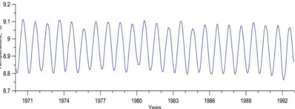
Simulation shows rather significant interannual variability of temperature field. Even av-eraged over the basin volume temperature demonstrates changes of annual minimums and maximums in the range of 0.05◦C (Fig. 1). Figure 1 shows that the basin-average temperature was minimal in winter of 1993 whereas the highest basin-averaged winter

(9)

OSD

9, 2039–2080, 2012

Title Page

Tables Figures

◭ ◮

Back Close

Full Screen / Esc

Discussion

P

a

per

|

Dis

cussion

P

a

per

|

Discussion

P

a

per

|

Discussio

n

P

a

per

temperature was in 1981. Lowest summer maximum was observed in 1976 year and highest in 1981 and 1984 years.

Such characteristics of the thermohaline structure as the autumn-winter cooling and spring-summer heating of surface waters, formation of the upper mixed layer (UML) and the seasonal thermocline, renewal of the cold intermediate layer (CIL) and

forma-5

tion of a new CIL, decrease of cold reserve in CIL by autumn are resolved by model simulations.

The UML depths vary within 20–64 m (based on isotherms 7◦C). The increased thickness of the upper mixed layer (up to∼_{54 m) was observed in 1976, 1985, 1987,}

1989 and 1992. The maximal depth of the mixed layer (∼_{64 m) was marked in 1993}

10

which is known to be one of the coldest years of the 20th century.

The CIL upper and lower boundaries are identified based on location of isotherm 8◦C. The CIL thickness diminishes during spring-summer mainly due to deepening of its upper boundary resulting from the surface water heating, vertical advection and turbulent heat diffusion. The changes in vertical temperature structure below the CIL

15

follows the seasonal and interannual variability of CIL lower boundary.

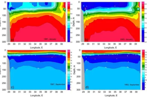
Following the classification suggested by (Titov, 2003), 1987 and 1989 are charac-terized by normal conditions whereas 1976, 1985, 1992 and 1993 corresponds to the cold winters. As shown in Fig. 2, during the cold winter of 1993 extreme cooling was on the sea surface and the CIL cold reserve as well as its thickness turned out to be

20

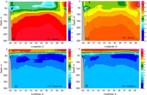
greater than in other years. Anomalously high heat fluxes on the air-sea boundary in winter also influence CIL behavior. In particular average temperature on all levels in the layer 0–300 m in autumn exceeds 8◦C in 1971, 1972, 1975, 1977, 1980–1982 and 1984 which is the result of considerable total heat inflow. The CIL continuity was vio-lated on some levels in these years (Fig. 3). On the whole the CIL thickness tended to

25

increase in 1985–1994.

(10)

OSD

9, 2039–2080, 2012

Title Page

Tables Figures

◭ ◮

Back Close

Full Screen / Esc

Discussion

P

a

per

|

Dis

cussion

P

a

per

|

Discussion

P

a

per

|

Discussio

n

P

a

per

|

warm 1981 on the level 50 m exceeded climatic values during almost the whole year (except for October–December). In cold 1993 year the temperature in the course of a seasonal cycle was much lower than the climatic one.

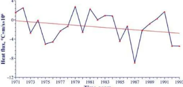
Analysis of tendencies of interannual variability of the temperature average over a year reveals the following (Fig. 4). In the layers 0–50 and 50–100 m linear trends

5

of variability are negative that agrees with the tendency of variability of annual average total heat flux. An average temperature decrease in those layers is equal−_2.57×₁₀−2

and−_1.03×₁₀−2◦_{C yr}−1_{, respectively. Rather weak, but positive trend is observed in the}

layer 100–300 m. An average temperature is characterized by a pronounced positive trend in deeper layers (500–1000 m).

10

Temperature in the Black Sea is influenced by many factors: heat fluxes through the surface and lateral sea boundaries; horizontal and vertical mixing; convection and wind mixing in autumn-winter period; summer upwelling and others. To study long-term variability of the vertical stratification we calculated differences between annual temperature and salinity values averaged on horizons 100 and 50 m, and also on levels

15

200 and 50 m in the maximally stratified part of pycnocline. On the whole the noted temperature differences increased in 1971–1993, and salinity differences – in 1971– 1985. Evident temperature increase on horizon 200 m and deeper can be explained by strengthening of stratification and decrease of the heat flux through the layer of high density gradients. The same results were obtained in (Belokopytov and Shokurova,

20

2005) at studying of decadal variability of di_fference between the averaged values of temperature and salinity on the same levels in 1970–1990.

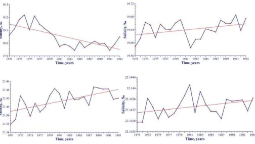
3.2 Interannual and seasonal variability of salinity

An averaged over the basin volume salinity also shows visible changes mainly on in-terannual scale (Fig. 5). Seasonal cycle does not manifested clearly probably because

25

the deep salinity is controlled by the lower Bosphorus current.

(11)

OSD

9, 2039–2080, 2012

Title Page

Tables Figures

◭ ◮

Back Close

Full Screen / Esc

Discussion

P

a

per

|

Dis

cussion

P

a

per

|

Discussion

P

a

per

|

Discussio

n

P

a

per

in the upper layer with thickness∼₁₀−_{20 m. In 1976 (cold winter conditions) average}

over the sea surface value of salinity was maximal and equal 18.4 ‰. The salinity of surface water diminishes noticeably starting from 1977. Based on climatic data and those on separate years, maximal salinity in its seasonal variation falls on February. Minimal salinity is observed in the late June and is a result of spring river floods; from

5

July salinity of surface waters begins to grow.

Analysis of tendencies of interannual variability of the layer-average salinity permitted to reveal the following regularities (Fig. 7). Negative linear salinity trend is observed in the upper part of halocline (0–20 m). The characteristic of the trend is equal to−_0.89×

10−2‰ yr−1. Tendency of the layer-average salinity in permanent halocline (20–150 m)

10

is opposite to that observed in the layer 0–20 m. The increase of average salinity in the layer 20–150 m achieves 0.16×₁₀−2_{‰ yr}−1_{. The local salinity minimum is distinguished}

in 1982 on a general positive tendency.

Interannual salinity variability in the layers 150–300 and 500–1000 m is characterized by positive linear trends with inclinations 0.24×₁₀−2_{and 0.2}×₁₀−4_{‰ yr}−1_{, respectively.}

15

A general positive tendency of salinity variation in the layer 150–300 m is accompanied by three local maximums in 1973, 1980 and 1988 years. Major contribution to the inter-annual variability of volume-average salinity is brought by the interannual salinity variability in a permanent halocline.

Temporal variability of annual mean salinity in the upper layer is defined by many

20

factors: water exchange through the Bosporus and the Kerch strait; rivers’ inflows; pre-cipitations; evaporation; intensity of seawater mixing in winter period by the convective and wind mixing. Freshwater balance had a positive linear trend in 1951–1985 (Hy-drometeorology and hydrochemistry, 1991). According to Lipchenko et al. (2006) in 1951–1995 evaporation decreased. The atmospheric precipitations (in annual values)

25

(12)

OSD

9, 2039–2080, 2012

Title Page

Tables Figures

◭ ◮

Back Close

Full Screen / Esc

Discussion

P

a

per

|

Dis

cussion

P

a

per

|

Discussion

P

a

per

|

Discussio

n

P

a

per

|

in 1951–1995. Exactly this factor explains negative tendency of temporal variability of annual salinity values in the upper layer 0–50 m.

Interannual variability of salinity in the Black Sea in a permanent halocline mainly depends on temporal variability of discharges and salinity of the Marmara Sea waters flowing to the sea through the Bosporus strait. By present there is no reliable

infor-5

mation about interannual variability of the mentioned above factors. Salinity increase below 50 m can be related to the positive salinity trend in the Mediterranean Sea (Thim-plis et al., 2004). Intensification of the deep water upwelling on the lower boundary of permanent halocline resulted in its rise is also possible reason of salinity increase in the upper layers and observed sharpening of pycnocline in 1971–1985.

10

3.3 Interannual and seasonal variability of the basin-scale circulation

Seasonal variability of kinetic energy during a year is definitely traced (Fig. 8). It is substantially lower in summer than in winter. The highest intensity of water circulation in the layer 0–300 m is observed in February–March, the lowest – in September–October. It is known that wind is a leading factor in formation of the Black Sea currents (Korotaev,

15

et al., 2001). Peculiarities of seasonal variability of the average over the sea surface wind stress vorticity are conditioned the seasonal variability of the averaged KE.

Interannual variability of annual mean, layers-averaged KE is characterized by the positive linear trends in the layers 0–50 and 50–150 m. The trends have the following characteristics: 3.41×₁₀−6_{and 3.49}×₁₀−6_M2_c−2_yr−1_{, respectively. The KE is}

dimin-20

ished by 1.25×₁₀−6_M2_c−2_yr−1_{in the layer 200–300 m.}

Changes of kinetic energy on the levels 50, 75, 100 and 150 m show the years with its lower (1974, 1978, 1980, 1983, 1986 and 1990) and higher (1972, 1977, 1981, 1988, 1991 and 1993) annual values. Intensity of winter water circulation in these years de-creased or inde-creased, respectively. The maps of currents for the years of stronger

circu-25

(13)

OSD

9, 2039–2080, 2012

Title Page

Tables Figures

◭ ◮

Back Close

Full Screen / Esc

Discussion

P

a

per

|

Dis

cussion

P

a

per

|

Discussion

P

a

per

|

Discussio

n

P

a

per

4 Evolution of the Black Sea ecosystem

Evolution of the annual-mean phytoplankton biomass in the upper 50 m layer derived from the modeling for the deep part of the Black Sea basin and North Western Shelf is shown in Fig. 9. In the deep part of the basin phytoplankton biomass increased ap-proximately twice from about 1.2 gC m−2in early seventies to 2 gC m−2during the early

5

1980s that prevailed throughouıt the 1980s and the early 1990s and then experienced a declining trend. On the northwestern shelf the level of the phytoplankton biomass in general is about one and half times as large as in the deep part of the basin. It also increased from about 2 gC m−2during the early seventies to 3 gC m−2in the mid-eighties. Then it decreased back to 2 gC m−2 until 1994 followed by an abrupt rising

10

during the rest of the 1990s. In general the phytoplankton biomass was higher in the western interior basin during the 1970s and the early1980s due to lateral support from the northwestern shelf. This excess biomass however became negligible during the reduced phytoplankton production phase of the northwestern shelf during 1985–1995. Interannual variability of the zooplankton biomass in the upper 50 m layer as a result

15

of the modeling is represented separately for the deep part of the Black Sea basin and North Western Shelf region in Fig. 10. In response to the phytoplankton biomass in-crease in deep part of the basin, zooplankton biomass inin-creased from about 0.8 gC m−2 in early seventies to about 1.1 gC m−2 in 1987. Then zooplankton biomass reduced rapidly in 1998 and stabilizes on the level of about 0.7 gC m−2. Zooplankton biomass on

20

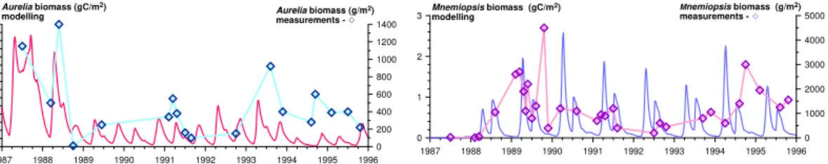
the northwestern shelf was retained uniform about 1.2 gC m−2until 1987, and reduced abruptly as well to about 0.7 gC m−2. This sudden decrease in zooplankton population in late eighties was caused by the population outbreak of Mnemiopsis leidyi all over the Black Sea. TheMnemiopsis leidyi invasion during 1989–1991 altered the previous carnivore predation ofAurelia aurita(Fig. 11).

25

(14)

OSD

9, 2039–2080, 2012

Title Page

Tables Figures

◭ ◮

Back Close

Full Screen / Esc

Discussion

P

a

per

|

Dis

cussion

P

a

per

|

Discussion

P

a

per

|

Discussio

n

P

a

per

|

Nitrate concentration in this layer then decreased to about 4 mmol N m−3in late 1990s– early 2000s due to the reduction in the anthropogenic nutrient supply (Konovalov and Murray, 2001). Apart from an increase in the value of the nitrate maximum by about three times during 20 yr (from the early 1970s until the end of 1980s) the position of ni-trate peak shifted by about 10 m upward. During winter season the nini-trate accumulated

5

in the upper layer due to intense winter mixing and then assimilated by phytoplankton once the spring warming initiated.

Figure 12 demonstrates variability of the basin-averaged surface phytoplankton and nitrate concentrations computed by the model in the deep part of the Black Sea to-gether with its concentration in the layer of nitrate maximum (dots). The annual-mean

10

surface nitrate concentration increased five times from 0.4 mmol N m−3in the early sev-enties to about 2.5 mmol N m−3in the early nineties, and then it decreased later by half. The surface phytoplankton concentration also increased from from 0.2 mmol N m−3 dur-ing the early 1970s to from 0.7 mmol N m−3in 1991. Then it reduced to 0.3 mmol N m−3. Both the surface nitrate concentration and the surface phytoplankton biomass followed

15

closely the changes in the concentration of nitrate maximum layer.

On the northwestern shelf of the Black Sea, nutrient concentrations were influenced mainly by the supply from the rivers (mainly Danube which provided about 70 % of total nutrient) (see Fig. 13, left). The surface phytoplankton biomass changed around 1.1 mmol N m−3 during the first twenty years, and declined abruptly during 1992–1994

20

and increased afterwards. But no clear correlation is evident with the anthropogenic nutrient supply as in the case of surface nitrate. It seems to be due to the fact that phytoplankton production was limited by other factors that the nitrate concentration in the northwestern shelf.

In more details, well-pronounced winter peaks of the basin-averaged surface nitrate

25

(15)

OSD

9, 2039–2080, 2012

Title Page

Tables Figures

◭ ◮

Back Close

Full Screen / Esc

Discussion

P

a

per

|

Dis

cussion

P

a

per

|

Discussion

P

a

per

|

Discussio

n

P

a

per

becomes at negligible quantities until the next winter. Apart from the seasonal changes, interannual variability of the nitrate and phytoplankton peaks is also well pronounced in Fig. 14. Their values are more clearly depicted in Fig. 15. From the early-1970s to the early 1990s, the winter nitrate maximum increases by about four times from 2 mmol N m−3to 8 mmol N m−3. Then it decreases to the value of about 3 mmol N m−3.

5

The mean spring phytoplankton biomass closely follows the winter nitrate concentra-tion, and rises from 0.35 mmol N m−3 in 1971 to 0.9 mmol N m−3 in 1991. Afterwards they tend to switch to the declining trend.

The changes in the Black Sea ecosystem during time period from 1971 until 2001 are visible not only in interannual changes of the main ecosystem components, but also

10

in their seasonal variability. The natural phytoplankton annual cycle of the spring and autumn blooms, as typical for the pre-eutrophication phase of the Black Sea ecosys-tem, has been replaced by a more complicated seasonal structure identified by several maxima, as illustrated by, the phytoplankton, zooplankton and medusaAurelia aurita changes in the upper 100 m layer in the central part of the basin for 1972, 1982 and

15

1992 in Fig. 16. In 1972, the phytoplankton annual cycle involved only the spring and autumn maxima in biomass. The zooplankton peak followed closely that of phytoplank-ton with some time lag of about half a month. The jellyfishAurelia auritaacquired two pronounced maxima in April–May and late autumn. In 1982 (the intense eutrophication phase), the phytoplankton annual cycle included additional peaks. Phytoplankton

expe-20

rienced a major bloom during the late winter-early spring season that was first followed by a zooplankton bloom of comparable intensity, which reduced the phytoplankton stock to a relatively low level, and then by anAurelia bloom in the late spring early summer that similarly reduced the zooplankton biomass. Subsequently, phytoplankton biomass recovered and produceed a relatively weak late spring bloom. TheAurelia population

25

produced a second peak in September–November and were accompanied by relatively high biomass of phytoplankton and zooplankton.

(16)

OSD

9, 2039–2080, 2012

Title Page

Tables Figures

◭ ◮

Back Close

Full Screen / Esc

Discussion

P

a

per

|

Dis

cussion

P

a

per

|

Discussion

P

a

per

|

Discussio

n

P

a

per

|

Mnemiopsis community. The sudden increase in Mnemiopsis population led to a re-duction in zooplankton biomass as well as an abrupt decline in the Aurelia biomass. Phytoplankton produced a set of maxima with the summer one is being the most-pronounced. The largest growth of the zooplankton was observed during mid-spring.

Apart from the bottom-up and top-down controls, intensity of the primary production

5

in the euphotic zone depends also on climatic conditions. The upper layer in deep part of the Black Sea is supplied with nutrients mainly by the winter mixing, the intensity of which depends on the severity and frequency of winter storms and cooling. The lower winter temperature is therefore associated with deeper winter convection and, as a result, more nutrient entrainment from its subsurface pool. Figure 17a displays

10

the basin-averaged annual-mean and winter-mean sea surface temperature changes obtained from the results of the hydrodynamic model. During the first phase (1971– 1993), both the annual and winter-mean temperature tended to have a declining trend (i.e. cooling) until their minimum in 1992 and 1993. Then they switched to the warming trend with the SST rise of about 2◦C from 1993 to 2001. In addition an opposite

corre-15

lation between winter surface nitrate concentration and winter-mean SST is evident in Fig. 17b. More details on the process of upper layer enrichment in winter season can be illustrated by the long-term changes in water column nitrate concentration during 1988–1994 at a location chosen from the interior Black Sea (Fig. 18). The most pro-nounced feature is an increase in the surface layer nitrate concentration due to higher

20

rate of input from nitracline due to intense winter mixing. The coldest winters in 1992 and 1993 provided the highest intensity winter surface nitrate concentration.

Satellite color scanners provide a good opportunity to validate the modeling results. For example, Fig. 19 compares the basin averaged surface chlorophyll concentration for the deep part of the basin derived from the modeling (solid line) and the

SeaW-25

(17)

OSD

9, 2039–2080, 2012

Title Page

Tables Figures

◭ ◮

Back Close

Full Screen / Esc

Discussion

P

a

per

|

Dis

cussion

P

a

per

|

Discussion

P

a

per

|

Discussio

n

P

a

per

tendency) or the changes in trophic interactions during the post-eutrophication phase of the ecosystem. Nevertheless, the model predicts a annual-mean surface chlorophyll concentration reasonably well and close to that given by the SeaWiFS data. Compari-son of seaCompari-sonal composite images of the surface chlorophyll provided by the SeaWiFS data and results of the modeling is shown in Fig. 20. The averaging was done over

5

four year time period 1998–2001. As indicated above, the model underestimated the autumn and winter concentrations and vice versa for the spring period. In summer, the di_fference is most observed in eastern part of the Black Sea.

The annual-averaged maps of surface chlorophyll for four years (1998–2001) pre-sented in Fig. 21 reveal highest chlorophyll concentration within the northwestern shelf.

10

Relatively high concentrations are also observed along the periphery of the basin due to the advection from the source in the northwestern shelf by the coastal current system of the basin scale cyclonic circulation. The mean level of surface chlorophyll derived from model agrees well with the SeaWiFS data, except the northwestern shelf where the model produces a wider coverage of high chlorophyll concentration coastal zone. It

15

may be due to the crude resolution of very complex trophic interactions by the model.

5 Discussion

The 3-D ecological model simulations presented here displayed the main features of the long-term (1971–2001) pelagic Black Sea ecosystem characteristics fairly well. The phytoplankton biomass was shown to increase from the early 1970s to the early 1990s

20

that represented the eutrophication phase of the Black Sea ecosystem. The surface phytoplankton biomass in the deep part of the basin increased by about 3 times. Zoo-plankton concentration also increased until the end of 1980s when the Mnemiopsis invasion caused a sudden reduction in the zooplankton community. These changes in the food web structure followed the changes in vertical chemical structure

charac-25

(18)

OSD

9, 2039–2080, 2012

Title Page

Tables Figures

◭ ◮

Back Close

Full Screen / Esc

Discussion

P

a

per

|

Dis

cussion

P

a

per

|

Discussion

P

a

per

|

Discussio

n

P

a

per

|

scanner measurements was quite satisfactory except a shift of the spring bloom to the winter during the late 1990s. Reasonably good consistency between the model simu-lations and the general knowledge of the Black Sea ecosystem changes inferred from the available data during last three decades of the 20th century suggests the critical importance of winter vertical mixing and advection processes that govern the amount

5

of nutrient supply into the euphotic zone and the subsequent intensity of plankton pro-duction. This climate-related process was further supported by the changes in the sea surface temperature. The intensity of upward nutrient flux is also related to the long-term accumulation of nitrate into the nitracline layer during the intense eutrophication phase. Majority of interannual changes in phytoplankton biomas may be explained by

10

nitrate concentration in the nitracline. Our simulations do not however provide a direct link between the nutrient supply from the River Danube and the intensity of phytoplank-ton blooms within the interior basin. The Danube influence on the nutrient supply was limited to the northwestern shelf TheMnemiopsispopulation outbreak was manifested mainly by the suppression of the zooplankton community and some shifts on the timing

15

of phytoplankton blooming periods, but its contribution to the phytoplankton commu-nity appears to be weaker than that predicted by the one-dimensional counterpart of the model (see Oguz et al., 2001). The model used in the present work appears to simulate the observed characteristic features of the intense eutrophication phase rea-sonably well, but not equally well for the post-eutrophication phase. It is related to the

20

transient character of the Black Sea ecosystem that keeps changing at a decadal time scale under different environmental perturbations and external stressors. It points to the necessity of some modifications in the physiological characteristics of the model as well as the food web interactions and feedback processes to coup with these exter-nal changes such as climatic warming, and changes in bottom-up control and trophic

25

(19)

OSD

9, 2039–2080, 2012

Title Page

Tables Figures

◭ ◮

Back Close

Full Screen / Esc

Discussion

P

a

per

|

Dis

cussion

P

a

per

|

Discussion

P

a

per

|

Discussio

n

P

a

per

References

Belokopytov, V. N. and Shokurova, I. G.: Estimation of temperature and salinity interdecadal variability in the Black Sea during time period 1951–1995, Ecological safety of coastal and shelf zone and complex use of their resources, 12, 12–21, 2005 (in Russian).

Blumberg, A. F. and Mellor, G. L.: A description of a three-dimensional coastal ocean model,

5

three dimensional shelf models, Coast. Estuar. Sci., 5. 1–16, 1987.

Dorofeyev, V. L.: Modeling of the decadal evolution of the Black Sea ecosystem, Mar. Hy-drophys. J., 6, 71–81, 2009 (in Russian).

Dorofeyev, V. L. and Korotaev, G. K.: Satellite altimetry assimilation in eddy-resolved model of the Black Sea circulation, Ukr. J. Mar. Res., 1, 52–68, 2004.

10

Simonov, A. I. and Altman E. N.: Hydrometeorology and hydrochemistry of the seas surrounded USSR, Gidrometeoizdat, St. Petersburg, 240 pp., 1991.

Gandin, L. S. and Kagan, R. A.: Statistical methods for interpretation of the meteorological data, Gidrometeoizdat, Leningrad, 357 pp., 1976 (in Russion).

Gregoire, M. and Friedrich, J.: Nitrogen budget of the North-Western Black Sea shelf as inferred

15

from modeling studies and in-situ benthic measurements, Mar. Ecol. Progr. Ser. 270, 15–39, 2004.

Gregoire, M. and Lacroix, G.: Exchange processes and nitrogen cycling on the shelf and con-tinental slope of the Black Sea basin, Global Biogeochem. Cy., 17, 4201–4217, 2003. Gregoire, M., Nezlin, N., Kostianoy, A., and Soetaert, K.: Modeling the nitrogen cycling and

20

plankton productivity in an enclosed environment (the Black Sea) using a three-dimensional coupled hydrodynamical – ecosystem model, J. Geophys. Res., 109, C05007, 2004. Gregoire, M., Raick, C., and Soetaert, K.: Numerical modeling of the Central Black Sea

ecosys-tem functioning during the eutrophication phase, Progr. Oceanogr., 76, 286–333, 2008. Konovalov, S. K. and Murray J. W.: Variations in the chemistry of the Black Sea on a time scale

25

of decades (1960–1995), J. Mar. Syst., 31, 217–243, 2001.

Knysh, V. V., Kubryakov, A. I., Moiseenko, V. A., Belokopytov, V. N., Inyushina, N. V., and Ko-rotaev, G. K.: Trends in thermohaline and dynamical characteristics of the Black Sea as a result of reanalysis for time period 1985–1994, Ecological safety of coastal and shelf zone and complex use of their resources, 16, 279–290, 2008 (in Russian).

30

(20)

OSD

9, 2039–2080, 2012

Title Page

Tables Figures

◭ ◮

Back Close

Full Screen / Esc

Discussion

P

a

per

|

Dis

cussion

P

a

per

|

Discussion

P

a

per

|

Discussio

n

P

a

per

|

Korotaev, G. K., Oguz, T., Nikiforov, A. A., and Koblinsky, C. J.: Seasonal, interannual and mesoscale variability of the Black Sea upper layer circulation derived from altimeter data, J. Geophys. Res., 108, 3122, doi:10.1029/2002JC001508, 2003.

Wright, D. G., Pawlowicz, R., McDougall, T. J., Feistel, R., and Marion, G. M.: Absolute Salinity, “Density Salinity” and the Reference-Composition Salinity Scale: present and future use in

5

the seawater standard TEOS-10, Ocean Sci., 7, 1–26, doi:10.5194/os-7-1-2011, 2011. Mellor, G. L. and Yamada, T.: Development of a turbulence closure model for geophysical fluid

problem, Rev. Geophys. Spase Phys., 20, 851–875, 1982.

Lancelot, C., Staneva, J., Van Eeckhout, D., Beckers, J., and Stanev, E.: Modelling the danube-influenced north-western continental shelf of the Black Sea. II: ecosystem response to

10

changes in nutrient delivery by danube river after its damming in 1972. Estuar. Coast. Shelf Sci., 54, 473–499, 2002.

Lipchenko, A. E., Ilyin, Y. P., Repetin, L. I., and Lipchenko M. M.: Decrease of evaporation from the Black Sea surface in the second half of the 20th century as a result of the global climate changes, Ecological safety of coastal and shelf zone and complex use of their resources, 14,

15

449–461, 2006 (in Russian).

Ludwig W.: River runoffand nutrient load data synthesis for hindcasting simulations, Deliverable 4.3.2, SESAME project, 2007.

Moiseenko, V. A. and Belokopytov, V. N.: Quality control of the hydrological data prepared for reanalysis of the Black Sea state during the time period of 1971–1993, Ecological safety of

20

the coastal zone and complex use of the shelf resources, 16, 184–189, 2008.

Moiseenko, V. A., Korotaev, G. K., Knysh, V. V., Kubryakov, A. I., Belokopytov V. N., and In-yushina, N. V.: Interannual variability of the thermohaline and dynamical characteristics of the Black Sea according to reasults of the reanalysis for time period 1971–1993, Ecological safety of the coastal zone and complex use of the shelf resources, 19, 216–227, 2009 (in

25

Russian).

Oguz, T., Ducklow, H. W., and Malanotte-Rizzoli P.: Modeling distinct vertical biochemical struc-ture of the Black Sea: dynamical coupling of the oxic, suboxic, and anoxic layers, Global Biochem. Cy., 14, 4, 1331–1352, 2000.

Oguz, T., Ducklow, H. W., Purcell, J. E., and Malanotte-Rizzoli P.: Modeling the response of

30

(21)

OSD

9, 2039–2080, 2012

Title Page

Tables Figures

◭ ◮

Back Close

Full Screen / Esc

Discussion

P

a

per

|

Dis

cussion

P

a

per

|

Discussion

P

a

per

|

Discussio

n

P

a

per

Oguz, T., Salihoglu, B., and Fach, B.: A coupled plankton-anchovy population dynamics model assessing nonlinear controls of anchovy and gelatinous biomass in the Black Sea, Mar. Ecol. Prog. Ser., 369, 229–256, 2008.

Purcell, J. E., Shiganova, T. A., Decker, M. B., and Houde, E. D.: The ctenophore mnemiopsis in native and exotic habitats: US estuaries versus the Black Sea basin, Hydrobiologia, 451,

5

145–176, 2001.

Repetin, L. I., Dolotov, V. V., and Lipchenko, M. M.: Space, temporal and climatic variability of the atmospheric precipitation over the Black Sea region, ecological safety of coastal and shelf zone and complex use of their resources, Sevastopol, 14, 462–476, 2006 (in Russian). Staneva, J. V. and Stanev, E. V.: Oceanic response to atmospheric forcing derived from different

10

climatic data sets, intercomparison study for the Black Sea, Oceanol. Ac., 21, 3, 383–417, 1998.

Titov, V. B.: Influence of climatic multiannual variability on the hydrological structure and inter-annual renewal of the cold intermediate layer in the Black Sea, Oceanology, 43, 176–184, 2003 (in Russian).

15

(22)

OSD

9, 2039–2080, 2012

Title Page

Tables Figures

◭ ◮

Back Close

Full Screen / Esc

Discussion

P

a

per

|

Dis

cussion

P

a

per

|

Discussion

P

a

per

|

Discussio

n

P

a

per

|

(23)

OSD

9, 2039–2080, 2012

Title Page

Tables Figures

◭ ◮

Back Close

Full Screen / Esc

Discussion

P

a

per

|

Dis

cussion

P

a

per

|

Discussion

P

a

per

|

Discussio

n

P

a

per

Fig. 2.Vertical sections of the temperature field along 43◦30′N in January (upper row) and

(24)

OSD

9, 2039–2080, 2012

Title Page

Tables Figures

◭ ◮

Back Close

Full Screen / Esc

Discussion

P

a

per

|

Dis

cussion

P

a

per

|

Discussion

P

a

per

|

Discussio

n

P

a

per

|

Fig. 3.Vertical sections of the temperature field along 43◦30′N in January (upper row) and

(25)

OSD

9, 2039–2080, 2012

Title Page

Tables Figures

◭ ◮

Back Close

Full Screen / Esc

Discussion

P

a

per

|

Dis

cussion

P

a

per

|

Discussion

P

a

per

|

Discussio

n

P

a

per

Fig. 4.Interannual variability of averaged over the sea surface of total heat flux from atmosphere

(26)

OSD

9, 2039–2080, 2012

Title Page

Tables Figures

◭ ◮

Back Close

Full Screen / Esc

Discussion

P

a

per

|

Dis

cussion

P

a

per

|

Discussion

P

a

per

|

Discussio

n

P

a

per

|

(27)

OSD

9, 2039–2080, 2012

Title Page

Tables Figures

◭ ◮

Back Close

Full Screen / Esc

Discussion

P

a

per

|

Dis

cussion

P

a

per

|

Discussion

P

a

per

|

Discussio

n

P

a

per

Fig. 6.Salinity sections along 43◦30′N in 1076 (upper panel) and 1984 (bottom panel) years

(28)

OSD

9, 2039–2080, 2012

Title Page

Tables Figures

◭ ◮

Back Close

Full Screen / Esc

Discussion

P

a

per

|

Dis

cussion

P

a

per

|

Discussion

P

a

per

|

Discussio

n

P

a

per

|

м м

Fig. 7.Interannual variability of salinity averaged in the layer – 20 m(a), 20–150 m (b), 150–

300 m(c), 500–1000 m(d).

(29)

OSD

9, 2039–2080, 2012

Title Page

Tables Figures

◭ ◮

Back Close

Full Screen / Esc

Discussion

P

a

per

|

Dis

cussion

P

a

per

|

Discussion

P

a

per

|

Discussio

n

P

a

per

|

Fig. 8.Interannual and seasonal variability of a volume averaged kinetic energy.

(30)

OSD

9, 2039–2080, 2012

Title Page

Tables Figures

◭ ◮

Back Close

Full Screen / Esc

Discussion

P

a

per

|

Dis

cussion

P

a

per

|

Discussion

P

a

per

|

Discussio

n

P

a

per

|

1970 1972 1974 1976 1978 1980 1982 1984 1986 1988 1990 1992 1994 1996 1998 2000 2002 0.8

1.2 1.6 2 2.4

2.8 Annual-mean phytoplankton biomass in the upper 50m layer (gC/m₍ 2) - the whole basin,

1970 1972 1974 1976 1978 1980 1982 1984 1986 1988 1990 1992 1994 1996 1998 2000 2002 2

2.2 2.4 2.6 2.8 3

3.2 Annual-mean phytoplankton biomass in the upper layer (coastal zone) (gC/m

2)

- western part, - eastern part).

Fig. 9.Evolution of the annual-mean phytoplankton biomass in the upper 50 m layer for the

(31)

OSD

9, 2039–2080, 2012

Title Page

Tables Figures

◭ ◮

Back Close

Full Screen / Esc

Discussion

P

a

per

|

Dis

cussion

P

a

per

|

Discussion

P

a

per

|

Discussio

n

P

a

per

|

1970 1972 1974 1976 1978 1980 1982 1984 1986 1988 1990 1992 1994 1996 1998 2000 2002 0.4

0.6 0.8 1

1.2 Annual-mean zooplankton biomass in the upper 50m layer (gC/m**2)_{(deep part of the basin)}

1970 1972 1974 1976 1978 1980 1982 1984 1986 1988 1990 1992 1994 1996 1998 2000 2002 0.4

0.6 0.8 1 1.2

1.4 Annual- mean zooplankton biomass in the upper layer (coastal zone) (gC/m**2)

Fig. 10.Evolution of the annual-mean zooplankton biomass in the upper 50 m layer for the deep

part of the Black Sea basin (left) and North Western Shelf (right).

(32)

OSD

9, 2039–2080, 2012

Title Page

Tables Figures

◭ ◮

Back Close

Full Screen / Esc

Discussion

P

a

per

|

Dis

cussion

P

a

per

|

Discussion

P

a

per

|

Discussio

n

P

a

per

|

1987 1988 1989 1990 1991 1992 1993 1994 1995 1996 0

1 2 3

0 200 400 600 800 1000 1200 1400

Aurelia biomass (gC/m2)

modelling Aurelia measurements - biomass (g/m 2)

1987 1988 1989 1990 1991 1992 1993 1994 1995 1996 0

1 2 3

0 1000 2000 3000 4000 5000

Mnemiopsis biomass (gC/m2) modelling

Mnemiopsis biomass (g/m2) measurements - 

Fig. 11.Evolution of the Aurelia (left) and Mnemiopsis (right) biomass in the upper 50 m layer for

(33)

OSD

9, 2039–2080, 2012

Title Page

Tables Figures

◭ ◮

Back Close

Full Screen / Esc

Discussion

P

a

per

|

Dis

cussion

P

a

per

|

Discussion

P

a

per

|

Discussio

n

P

a

per

|

1970 1972 1974 1976 1978 1980 1982 1984 1986 1988 1990 1992 1994 1996 1998 2000 2002 0

1 2 3

2 3 4 5 6 7 8 9 10

Ann

Ann

ual-mean surface Nitrate concentration (mmol/m3)

 ual-mean nitrate concentration in the layer of maximum (mmol/m3)

Sur

fa

1970 1972 1974 1976 1978 1980 1982 1984 1986 1988 1990 1992 1994 1996 1998 2000 2002 0.2

0.3 0.4 0.5 0.6 0.7

2 3 4 5 6 7 8 9 10

A

A

nnual-mean surface phytoplankton concentration (mmol/m3) (Deep part of the basin)

nnual-mean nitrate concentration in the layer of maximum (mmol/m3)

Phytoplankton

Nitrate

c

e ni

tr

ate



 

Fig. 12.Annual-mean surface nitrate (left) and phytoplankton (right) concentrations (bars) in the

deep part of the Black Sea and annual-mean nitrate maximum (dots) (results of the modeling).

(34)

OSD

9, 2039–2080, 2012

Title Page

Tables Figures

◭ ◮

Back Close

Full Screen / Esc

Discussion

P

a

per

|

Dis

cussion

P

a

per

|

Discussion

P

a

per

|

Discussio

n

P

a

per

|

 





1970 1972 1974 1976 1978 1980 1982 1984 1986 1988 1990 1992 1994 1996 1998 2000 2002 8

12 16 20 24 28 32

500 600 700 800 900 1000 1100

Annual-mean surface Nitrate concentration (mmol/m3)

 Nitrate supply by Danube river (kt/y)

Su

1970 1972 1974 1976 1978 1980 1982 1984 1986 1988 1990 1992 1994 1996 1998 2000 2002 0.8

1 1.2 1.4

500 600 700 800 900 1000 1100

Annual-mean surface Phytoplankton concentration (mmol/m3) (NWS)

 Nitrate supply by Danube river (kt/y)

Phyt

oplankton Nitr

a

te

rfa

ce

n

it

ra

te

Fig. 13.Annual-mean surface nitrate (left) and phytoplankton (right) concentrations (derived

(35)

OSD

9, 2039–2080, 2012

Title Page

Tables Figures

◭ ◮

Back Close

Full Screen / Esc

Discussion

P

a

per

|

Dis

cussion

P

a

per

|

Discussion

P

a

per

|

Discussio

n

P

a

per

|

1970 1972 1974 1976 1978 1980 1982 1984 1986 1988 1990 1992 1994 1996 1998 2000 2002 0

1 2 3 4 5 6 7

8 _{Nitrate concentration (mmol N /m}3₎

1970 1972 1974 1976 1978 1980 1982 1984 1986 1988 1990 1992 1994 1996 1998 2000 2002 0

1 2 3

Phytoplankton concentration (mmol N /m3₎

 

t t

Fig. 14. Long-term evolution of the basin-averaged surface nitrate (left) and phytoplankton

(right) concentrations in the deep part of the Black Sea (results of the modeling).