Perturbed damped pendulum:
finding periodic solutions via averaging method
(Perturba¸c˜oes do pˆendulo amortecido: encontrando solu¸c˜oes peri´odicas via m´etodo “averaging”)Douglas D. Novaes
1Departamento de Matematica, Universidade Estadual de Campinas, Campinas, SP, Brasil
Recebido em 3/2/2012; Aceito em 15/12/2012; Publicado em 18/3/2013
Using the damped pendulum model we introduce the averaging method to study the periodic solutions of dy-namical systems with small non–autonomous perturbation. We provide sufficient conditions for the existence of periodic solutions with small amplitude of the non–linear perturbed damped pendulum. The averaging method provides a useful means to study dynamical systems, accessible to Master and PhD students.
Keywords: averaging method, periodic solutions, nonlinear systems, damped pendulum.
Utilizando o modelo do pˆendulo amortecido, introduzimos o m´etodo “averaging” no estudo de solu¸c˜oes peri´odicas de sistemas dinˆamicos com pequenas perturba¸c˜oes n˜ao autˆonomas. Considerando perturba¸c˜oes do sistema do pˆendulo amortecido, fornecemos condi¸c˜oes suficientes para a existˆencia de solu¸c˜oes peri´odicas de pequena amplitude. O m´etodo “averaging” fornece uma ferramenta ´util no estudo de sistemas dinˆamicos e ´e acess´ıvel a estudantes de p´os-gradua¸c˜ao.
Palavras-chave: m´etodo “averaging”, solu¸c˜oes peri´odicas, sistemas n˜ao lineares, pˆendulo amortecido.
1. Introduction
Systems derived from the pendulum give to students important and practical examples of dynamical sys-tems. For instance, we can see the weight-driven pen-dulum clocks which had its historical and dynamical aspects studied by Denny in a recent paper [1]. This system has been revisited by Llibre and Teixeira in [2], and using some simple techniques, from averaging the-ory, they got the same results. Usually, the systems involving pendulums have also been used to introduce mathematical concepts of classical mechanics, as we can see in Ref. [3].
In this paper we attempt to use a simple physical system, as the damped pendulum, to introduce some concepts and techniques of the important and useful averaging theory, which can be used to study the pe-riodic solutions of dynamical systems. For instance, in Ref. [4], Llibre, Novaes and Teixeira have used the averaging theory to provide sufficient conditions for the existence of periodic solutions of the planar double pen-dulum with small oscillations perturbed by non–linear functions.
2.
The damped pendulum
We consider a system composed of a point massm mo-ving in the plane, under gravity force, such that the
distance between the point massm and a given point Pis fixed and equal tol. We also consider that the mo-tion of the particle suffers a resistance propormo-tional to its velocity. This system is calledDamped Pendulum.
The position of the pendulum is determined by the angleθshown in Fig. 1. The equation of motion of this system is given by
¨
θ=−asin(θ)−bθ,˙ (1)
where a > 0 and b > 0 are real parameters, with a=g/l, g the acceleration of the gravity,l the length of the rod andbthe damping coefficient. We shall also assume that the damping coefficientb is a small para-meter.
There are many other kinds of resistance that the particle motion can suffer, providing many different dy-namical behaviors (see Remark 1). For instance, the Coulomb Friction introduces a discontinuous term in the equation of motion (1). For more details about this last issue, see the book of Andronovet al.[5].
In the qualitative theory of dynamical systems, a singularity x∗ of an autonomous differential system
˙
x(t) =F(x),i.e. F(x∗) = 0, is calledHyperbolic if the
eigenvalues of the linear transformationDF(x∗)
(deri-vative ofF inx∗) has non–zero real components. In this
case, applying the classical Hartman-Grobman Theo-rem(see Theorem 2.2.3 from Ref. [6]) we can study the local behavior of the system looking to the linearized
1E-mail: [email protected].
system ˙y(t) =D(x∗)y.
Figura 1 - Pendulum.
Remark 1. Here, the behavior of a dynamical system can be informally understood as how the phase portrait looks like. For a general introduction to qualitative the-ory of dynamical systems see for instance the book of Arrowsmith and Place [6].
The linearized equation of motion of the damped pendulum is given by
¨
θ=−aθ−bθ.˙ (2)
Considering the coordinates (θ,θ), the system (2)˙ has the following eigenvalues
λ1=−
b+√b2−4a
2 and λ2=
−b−√b2−4a
2 ,
which is the eigenvalues of the matrix
0 1
−a −b
.
Note that for b2 ≥ 4a the eigenvalues λ
1 and λ2 are both negative, then the singularity (θ,θ) = (0,˙ 0) is a attractor node, represented in the Fig. 2. Now, forb2<4aboth eigenvaluesλ
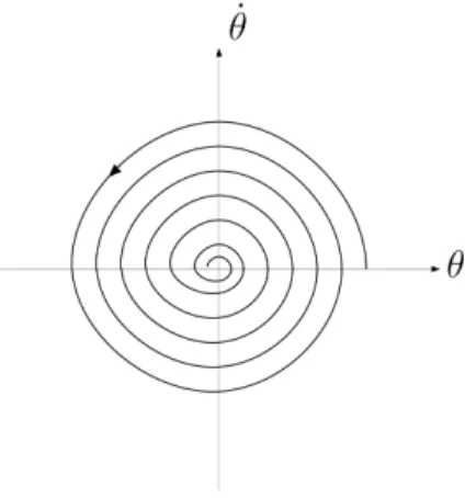
1 andλ2 have the imagi-nary part different of zero and negative real part, then the singularity (θ,θ) = (0,˙ 0) is a attractor focus, re-presented in the Fig. 3. Both cases are topologically equivalent.
Figura 2 - Attractor node.
Figura 3 - Attractor focus.
Observe that without the damping effect,i.e. b= 0, both eigenvaluesλ1andλ2would be purely imaginary, then the singularity (θ,θ) = (0,˙ 0) would be a center (which is a non–hyperbolic singularity), represented in the Fig. 4. This last case is not topologically equivalent to the two cases above.
Figura 4 - Center.
We emphasize here that, for b ̸= 0, the linearized Eq. (2) can only be used to study the local behavior, at (θ,θ) = (0,˙ 0), of the original (non–linear) system (1). However, a periodic solution of a differential system is a global element of the phase portrait. Thus to study these elements we have to consider the non–linear equa-tion, which has the global information of the system.
As we have seen, whenb̸= 0, the origin is an attrac-tor singularity, thus the orbits of the system starting sufficiently closer to the origin tends to it. In other words, the damped pendulum always tends to stop. The following study provide conditions to drop this re-gime obtaining thus a periodic solution of the system which never reaches the origin.
3.
Perturbed system
Let (f, g) be an ordered pair of functions, such that
We consider the non–autonomous perturbation of the system (1)
¨
θ=−asin(θ)−bθ˙+εf(t, θ,θ) +˙ ε2g(t, θ,θ).˙ (3)
By a non–autonomous perturbation we understand that the function (f, g)(t, θ,θ) is dependent of the varia-˙ blet. We also assume that the ordered pair of functions (f, g) satisfies the following conditions:
(C1) f(t, θ,θ) and˙ g(t, θ,θ) are˙ C2 functions;
(C2) f(t, θ,θ) and˙ g(t, θ,θ) are locally Lipschitz with˙ respect to (θ,θ);˙
(C3) f(t, θ,θ) and˙ g(t, θ,θ) are respectively˙ Tf andTg
periodic in the variablet with
Tf =
pf
qf
2π
√a and Tg=
pg
qg
2π
√a,
beingpi and qi relatively prime positive integers
fori=f, g;
(C4) and f(t,0,0) = 0.
We say that the Basic Conditionsare satisfied for an ordered pair of functions (f, g) (which define the non–autonomous perturbation on the system (3)) when (f, g) satisfies the conditions Ci, fori= 1,2,3,4.
Remark 2. For simplicity, instead condition C3 we can assume, without loss of generality, that the func-tions f(t, θ,θ)˙ and g(t, θ,θ)˙ are T–periodic with T = 2pπ/√afor some integer p. Indeed, taking p the least common multiple betweenpf andpg, we have that there
exists integers nf andng such that p=nfpf =ngpg.
Hence
p√2π
a =nfqf pf
qf
2π
√
a =ngqg pg
qg
2π
√
a.
4.
Change of coordinates
As we shall see in the Section 6. the main result from theAveraging Theory, used in this present work, assu-mes that the perturbed system is given in anStandard Form (8). To get it, we have to introduce two changes of coordinates. The first one is done in the following.
If we takeθ=εφwith|ε|>0, then the system (3) becomes
¨
φ=−asin(εφ)
ε −ε¯bφ˙+f(t, εφ, εφ) +˙ εg(t, εφ, εφ).˙ (4) Note that, since bis a small parameter, we can as-sume that b = ε¯b, with ¯b > 0 if we consider pertur-bations for ε > 0; and with ¯b < 0 if we consider per-turbations for ε < 0. Henceforward we assume that ε >0.
As a consequence of this coordinates change we have the following lemma.
⌋
Lemma 1. There exists a continuous function r(t, φ,φ, ε),˙ T–periodic in the variable t with T = 2pπ/√a, such that the system (4)is written as
¨
φ=−aφ+ε(g0(t) +f1(t)φ+ (f2(t)−¯b) ˙φ
)
+ε2r(t, φ,φ, ε),˙ (5) where
g0(t) =g(t,0,0), f1(t) = ∂f
∂θ(t,0,0), and f2(t) = ∂f
∂θ˙(t,0,0).
Demonstra¸c˜ao. Set the variables t,φand ˙φas the parameters of theC2 functions7→F(s;t, φ,φ) defined as˙
F(s;t, φ,φ) =˙ −asin(sφ)
s −s¯bφ˙+f(t, sφ, sφ) +˙ sg(t, sφ, sφ).˙
Applying the Taylor’s Formula with Lagrange Remainder for the functionF(s;t, φ,φ) at˙ s= 0 we conclude that there exists 0< h <1 such that
F(ε;t, φ,φ) =˙ F(0;t, φ,φ) +˙ ε F′(0;t, φ,φ) +˙ ε2F
′′(ε h;t, φ,φ)˙
2 ,
= −ax+ε(g0(t) +f1(t)φ+ (f2(t)−¯b) ˙φ
)
+ε2F′′(ε h;t, φ,φ)˙
2 .
Since
F′′(ε h;t, φ,φ) =˙ ε2ah φcos(ε hφ) +a(ε
2h2φ2−2) sin(ε hφ) ε3h3
+d 2 ds2
(
f(t, sφ, sφ) +˙ sg(t, sφ, sφ)˙ )
and
lim
ε→0
ε2ah φcos(ε hφ) +a(ε2h2φ2−2) sin(ε hφ)
ε3h3 =
ax3 3 . It follows that the function
r: (t, φ,φ, ε)˙ 7→F
′′(ε h;t, φ,φ)˙
2 is continuous in the variableε. By the other hand
r(t, φ,φ, ε) =˙ F(ε h;t, φ,φ) +˙ ax ε2 −
g0(t) +f1(t)φ+ (f2(t)−¯b) ˙φ
ε .
Thus we conclude that the function r(t, φ,φ, ε) is continuous in the variables˙ t ,φ and ˙φ, and T–periodic in the variablet.
⌈
TheTaylor’s Formula with Lagrange Remainderhas its statement and its proof done in the book of Lima [7]. To study the periodic solutions of the system (3) we shall study the periodic solutions of the system (5). Indeed, ifψ(t, ε) is a solution of system (5), then ϕ(t, ε) =εψ(t, ε) is a solution of the system (3). Howe-ver, the change of coordinate, introduced above, res-tricts our study only for periodic solutions close to the origin, since |ϕ(t, ε)| → 0 as ε→0 for t ∈I for every I compact interval of R. In this case, we say that this
periodic solution is bifurcating of the origin.
Now, denoting (x, y) = (φ,φ), the second order dif-˙ ferential Eq. (5) can be written as the first order diffe-rential system
˙ x=y,
˙
y=−ax+ε(
g0(t) +f1(t)x+ (f2(t)−¯b)y)+ε2r(t, x, y, ε). (6) Observe that the unperturbed system, i.e. ε = 0,
has the following eigenvalues
λ1=i√a and λ2=−i√a, thus it is a center at the origin, see Fig. 4.
There are many works which deal with perturbation of centers, even in higher dimensions. For instance we can see the paper of Llibre and Teixeira [8].
The second change of coordinates (13) will be done in the Section 7..
5.
Statements of the main results
Our main goal, in this present work, is to find suffici-ent conditions on the ordered pair of functions (f, g) to assure the existence of periodic solutions of the system (3). For this, we shall provide a matrixM such that its non–singularity, i.e. det(M)̸= 0, implies the existence of at least one periodic solution, for ε >0 sufficiently small, of the system (3). ⌋
We define the matrix M = (Mij)2×2as
M11=− ¯bπ
√
a+
∫ 2√pπ a
0
sin(√at)
( −cos(
√
at)
√
a f1(t) + sin(
√
at)f2(t)
)
dt,
M12=
∫ 2√pπ a
0
sin(√at) a
(
−sin(√at)f1(t)−√acos(√at)f2(t)
)
dt,
M21=
∫ 2√pπ a
0
cos(√at)(
cos(√at)f1(t)−√asin(√at)f2(t))dt,
M22=− ¯bπ
√
a+
∫ 2√pπ a
0
cos(√at)
(
sin(√at)
√
a f1(t) + cos(
√
at)f2(t)
)
dt.
(7)
Our main result on the periodic solutions of the damped pendulum with small non–autonomous pertur-bation (3) is the following.
Theorem 2. Assume that the Basic Conditions are satisfied for the pair of functions (f, g), which define the non–autonomous perturbation on the system (3). If det(M)̸= 0, then for ε >0 sufficiently small the per-turbed damped pendulum (3) has aT–periodic solution θ(t, ε), such that
(θ(0, ε),θ(0, ε))˙ →(0,0),
when ε→0.
Theorem 2 is proved in section 7.. Its proof is based in the averaging theory for computing periodic soluti-ons, which will be introduce in section 6..
We provide an application of Theorem 2 in the fol-lowing corollary.
Corollary 3. Assume that the Basic Conditions are satisfied for the pair of functions (f, g), which define the non–autonomous perturbation on the system (3). Moreover, suppose that
∂f
∂θ(t,0,0) =C1 and ∂f
∂θ˙(t,0,0) =C2. If (C1, C2)̸= (0,¯b), then there exists aT–periodic solu-tionθ(t, ε)of the perturbed damped pendulum (3), such that
(θ(0, ε),θ(0, ε))˙ →(0,0),
when ε→0.
The Corollary 3 will be proved in section 7..
6.
Averaging theory
We present in this section a basic result known asFirst Order Averaging Theorem. For a general introduction to averaging theory see for instance the book of Sanders and Verhulst [9] and the book of Verhulst [10].
We consider the differential equation
˙
X =ε F1(s, X) +ε2R(s, X, ε), (8) where F1 : R×U → Rn is a smooth function and R :R×U ×(−εf, εf)→Rn is a continuous function.
These functions are bothT-periodic in the first variable t andU is an open subset ofRn.
Remark 3. The Eq. (8) is the Standard Form, of a differential system, to apply the first order averaging theorem.
We define the averaged system associated to system (8) as
˙
Z(t) =f1(Z), (9)
wheref1:U →Rn is given by
f1(Z) =
∫ T
0
F1(s, Z)ds. (10)
In resume, the averaging theory gives a quantitative relation between the solutions of some non–autonomous differential system and the solutions of the averaged dif-ferential system, which is an autonomous one. In our case, as we are working with periodic systems, the ave-raging method also leads to the existence of periodic solutions.
The next theorem associates the singularities of the system (9) with the periodic solutions of the differential system (8).
Theorem 4. Assume that
(i) F1 andRare locally Lipschitz with respect to x; (ii) for a ∈ U with f1(a) = 0, there exist a
neigh-borhood V of a such that f1(Z) ̸= 0 for all z∈V\{a} anddet(df1(a))̸= 0.
Then, for |ε| > 0 sufficiently small, there exist a T-periodic solution X(t, ε) of the system (8) such that X(0, ε)→aasε→0.
Using Brower degree theory, the hypotheses of The-orem 4 becomes weaker. For a proof of TheThe-orem 4 see Buica and Llibre [11].
Remark 4. Using the Averaging Theorem 4 we can study some solutions of Eq. (8)only studying the alge-braic equationf1(Z) = 0, instead solving the differen-tial equation. This is one of the main characteristic of Averaging Theory.
7.
Proofs of Theorem 2 and Corollary 3
In order to use the Theorem 4 in the proof of Theorem 2, we have to modify the Eq. (6). If we denote
x=
x y
, A=
0 1
−a 0
,
F(t,x) =
0
g0(t) +f1(t)x+ (f2(t)−¯b)y
, (11)
and
R0(t,x) =
0
r(t,x, ε)
,
then the Eq. (6) can be written in the matrix form
˙
Take y(t)∈R2 as
y(t) =e−Atx(t), (13) where
eAt =
cos (√at) sin (
√
at)
√
a
−√asin (√at) cos (√at)
is the matrix of the fundamental solution of the un-perturbed differential system (12), i.e., ε = 0. This change of coordinates is done in the book of Sanders and Verhulst [12].
Observe that the applicationt7→e−AtisT–periodic
function with T = 2π/√a, since the eigenvalues of A are purely imaginary. Moreovery(0) =x(0).
Lemma 5. The system (12)is written in the new va-riabley as
˙
y=εF˜(t,y) +ε2R(t,˜ y, ε), (14) where ˜F(t,y) = e−AtF(t, eAty) and ˜R(t,y, ε) =
e−AtR
0(t, eAty, ε). Demonstra¸c˜ao.
˙
y(t) = d dt
(
e−Atx(t))
,
=−Ae−Atx(t) +e−Atx˙(t),
=−Ae−Atx(t) +e−At(Ax(t) +εF(t,x(t)) +
ε2R
0(t,x(t))),
=εe−AtF(t,x(t)) +ε2e−AtR
0(t,x(t)), =εe−AtF(t, eAty(t)) +ε2e−AtR
0(t, eAty(t)), =εF˜(t,y(t)) +ε2R(t,˜ y(t), ε).
Note that the system (14) is written in the standard form (8). Thus we are ready to prove the Theorem 2.
Proof of Theorem 2. The smooth functions f(t,x) and g(t,x) are T-periodic in the variable t, with T = 2pπ/√a, which implies that the smooth functions
˜
F(t,y) and ˜R(t,y, ε) are alsoT-periodic int.
We shall apply the Theorem 4 to the differential Eq. (14). Note that the Eq. (14) can be written as the Eq. (8) taking
X =y, F1(t, X) = ˜F(t,y),
and R(t, X, ε) = ˜R(t,y, ε). (15)
Observe that, by Lemma 1, the function F1 and R satisfy the assumptions of Theorem 4.
Given z∈R2, we can compute the averaged
func-tionf1:R2→R2, defined in (10), as
f1(z) =
∫ 2√pπ a
0
e−AtF(t, eAtz)dt, = Mz−v,
whereM is defined in (7) and
v=
∫ 2√pπ a
0
sin(√at)
√
a g0(t)dt
− ∫ 2√pπ
a
0
cos(√at)g0(t)dt
.
Assuming that det(M)̸= 0, we conclude that there exists a solution z0 = (x0, y0) of the linear system f1(z) = 0 given byz0 =M−1v which satisfies the hy-potheses of Theorem 4. Indeed
det(df1(z0)) = det(M)̸= 0.
Moreover, det(M) ̸= 0 also implies the uniqueness of the solution z0 of the systemMz=v, thus f1(z)̸= 0 for allz∈R2\{z0}.
Hence, applying Theorem 4, follows that there exists a T–periodic solution y(t, ε) of the system (14) such that
y(0, ε)→z0 whenε→0,
which implies the existence of a periodic solution (x(t, ε), y(t, ε)) of the system (6) such that
(x(t, ε), y(t, ε)) =x(t, ε) =eAty(t, ε).
Sincex(0) =y(0) it follows that
x(0, ε) y(0, ε) → x0 y0 ,
whenε→0. Hence
(
θ(t, ε),θ(t, ε)˙ )=ε(x(t, ε), y(t, ε))
is a T–periodic solution of the system (3) such that
(
θ(t, ε),θ(t, ε)˙ )→(0,0),
whenε→0.
Proof of Corollary 3. The hypotheses of Corollary 3 implies that M =
(C2−¯b)π
√
a −
C1π
√
a3 C1π
√
a
(C2−¯b)π
√ a . Thus
det(M) = (C 2
1+a(¯b−C2)2)π2 a2 .
8.
Simulation
Consider the following differential equation ¨
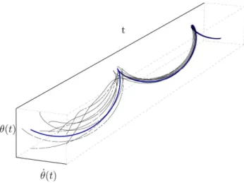
θ=−sin(θ)−εθ˙+ε2sin(t). (16) Observe that the Eq. (16) is a small perturbation of the damped pendulum system. Indeed, Eq. (3) becomes Eq. (16) by taking the parameters a = 1, and b = ε; and the functions f(t, θ,θ) = 0, and˙ g(t, θ,θ) = sin(t). Therefore, considering˙ C1 =C2 = 0 we can apply the Corollary 3 to assure the existence of a periodic solution of the system (16).
Indeed, proceeding with the numerical simulation we find this periodic solution, represented by the blue line in Fig. 5.
Figura 5 - Solutions converging to the periodic solution.
This simulation has been done using the Wolfram Mathematicar 8 software.
9.
Conclusions and future directions
The averaging theory is a collection of techniques to study, via approximations, the behavior of the soluti-ons of a dynamical system under small perturbatisoluti-ons. As we have seen, it can also be used to find periodic solutions.
In this paper, we have presented one of these tech-niques and used it to find conditions that assure the existence of a periodic solution of the non–autonomous perturbed damped pendulum system. In resume, we have got an algebraic non–homogeneous linear system Mz = v such that its solution, when det(M) ̸= 0, is associated with a periodic solution of such perturbed system.
Recently, Llibre et al. [13] have extended the ave-raging method for studying the periodic solutions of a class of differential equations with discontinuous second member. Therefore we are able to consider for instance equations of kind
¨
θ=−asin(θ)−bsign( ˙θ) +εf(t, θ,θ) +˙ ε2g(t, θ,θ).˙
Here, the term bsign( ˙θ) represents the Coulomb Fric-tion, where the function sgn(z) denotes the sign func-tion,i.e.
sgn(z) =
−1 ifz <0, 0 ifz= 0, 1 ifz >0.
For instance, in Ref. [14], Llibreet al. have used the averaging theory to provide sufficient conditions for the existence of periodic solutions with small amplitude of the non–linear planar double pendulum perturbed by smooth or non–smooth functions.
Acknowledgements
The author is supported by a FAPESP–BRAZIL grant 2012/10231–7.
References
[1] M. Denny, European Journal of Physics23, 449 (2002).
[2] J. Llibre and M.A. Teixeira, European Journal of Phy-sics31, 1249 (2010).
[3] G.A. Monerat, E.V. Corrˆea Silva, G. Oliveira-Neto, A.R.P. de Assump¸c˜ao and A.R.R. Papa, Revista Bra-sileira de Ensino de F´ısica28, 177 (2006).
[4] J. Llibre, D.D. Novaes and M.A. Teixeira, S˜ao Paulo J. Math Sciences5, 317 (2011).
[5] A.A. Andronov, A.A. Vitt and S.E. Khaikin, Theory of Oscillators, International Series of Monographs In Physics4, Pergamon Press, 1966.
[6] D.K. Arrowsmith and C.M. Place, An Introduction to Dynamical System (Cambridge University Press, 1990).
[7] E.L. Lima, An´alise Real Volume 1. Fun¸c˜oes de Uma Vari´avel (IMPA, 2008).
[8] J. Llibre and M.A. Teixeira, Journal of Dynamical and Differential Equations18, 931 (2006).
[9] J.A. Sanders and F. Verhulst, Applied Mathematical Sciences v. 59 (Springer, Berlin, 1985).
[10] F. Verhulst,Nonlinear Diferential Equations and Dy-namical Systems(Springer, Universitext, 1991). [11] A. Buic˘a and J. Llibre, Bull. Sci. Math.128, 7 (2004).
[12] J.A. Sanders and F. Verhulst, Applied Mathematical Sciences v. 59 (Springer, Berlin, 1985).
[13] J. Llibre, D.D. Novaes and M.A. Teixeira, ar-Xiv:1205.4211 [math.DS], http://arxiv.org/abs/ 1205.4211.