Simplified Modelling of Displacement Ventilation
Doutoramento em Energia e Ambiente
Especialidade em Energia e Desenvolvimento Sustentável
Nuno André Marques Mateus
Tese orientada por:
Professor Doutor Guilherme Carvalho Canhoto Carrilho da Graça
UNIVERSIDADE DE LISBOA
FACULDADE DE CIÊNCIAS
Simplified Modelling of Displacement Ventilation
Doutoramento em Energia e Ambiente
Especialidade em Energia e Desenvolvimento Sustentável
Nuno André Marques Mateus
Tese orientada por:
Professor Doutor Guilherme Carvalho Canhoto Carrilho da Graça
Júri: Presidente:
● Doutor João Catalão Fernandes (Faculdade de Ciências, Universidade de Lisboa) Vogais:
● Doutor Paul Linden (Faculty of Mathematics, University of Cambridge)
● Doutor Eusébio Zeferino da Conceição (Faculdade de Ciências e Tecnologia, Universidade do Algarve) ● Doutor João Manuel de Almeida Serra (Faculdade de Ciências, Universidade de Lisboa)
● Doutor Guilherme Carvalho Canhoto Carrilho da Graça (Faculdade de Ciências, Universidade de Lisboa) ● Doutora Marta João Nunes Oliveira Panão (Faculdade de Ciências, Universidade de Lisboa)
Acknowledgements
This work would not have been possible without the financial support of Calouste Gulbenkian Foundation through Ph.D. Grant No. 126724.
I am grateful to my supervisor professor Guilherme Carrilho da Graça, for having accepted to guide me, for all the opportunities he provided me and the challenges he put me through which allowed me to learn more than I could ever expected.
To Filipa Silva, Daniel Albuquerque, António Soares and all the other students that contributed for an incredibly friendly and supportive working atmosphere in the “buildings team”.
To all my friends, for the friendship and support.
To my parents, my sister and my family for always encouraging me to keep improving. To Luísa, who challenges me every days.
Finally, to Mariana, whom I admire deeply for being an example dedication and determination, and who always believed and encourage me.
Abstract
With the aim of creating adequate indoor conditions, modern buildings use energy for space heating, ventilation and air conditioning (HVAC). The environmental impact of this energy use creates an urgent need to develop strategies to reduce HVAC related energy consumption. This thesis contributes to this goal by testing and developing simplified models for highly efficient thermally stratified building displacement ventilation (DV) strategies. DV is characterized by thermal stratification that cannot be adequately modelled using the fully mixed room air approach that is common in overhead air conditioning system design. This thesis proposes a simplified approach for DV that models the room thermal stratification using three air temperature nodes: lower layer (floor level, 0.1m), occupied zone and upper mixed layer. The proposed approach is a development of one of the two models currently available in the open source thermal simulation tool EnergyPlus. A methodology for locating the neutral height in temperature profiles was developed. This methodology was used to verify the applicability of the Morton et al. (1956) plume flow equation to predict the neutral level in DV rooms. Detailed monitoring campaigns were carried out and the measurement results of several independent studies were analyzed in order to evaluate the performance of different DV systems configurations. The proposed model was successfully validated using thirty different full-scale experimental measurements in ten different room geometries, ranging from small laboratory test cells, classrooms, and a large concert hall. The model is able to simulate the air temperatures in the test cases with an average error of 5%, corresponding to a deviation of 0.4ºC. The experimental results show that the model provides significantly improved precision when compared to existing DV nodal models and demonstrate the ability of the three-node model to simulate DV systems in any of the configurations tested. The proposed model is simple and can be easily incorporated into a dynamic simulation program such as EnergyPlus.
Keywords
Resumo
Com o intuito de criar condições ambientais adequadas, os edifícios modernos utilizam a energia para aquecimento, ventilação e ar condicionado (AVAC). O impacto ambiental da utilização desta energia cria a necessidade urgente de desenvolver estratégias para reduzir o consumo de energia associada aos sistemas de AVAC. Esta tese contribui para esse objetivo através do desenvolvimento de modelos simplificados para o eficiente sistema de ventilação por deslocamento do ar (DV). Os sistemas DV são caracterizados pelo desenvolvimento da estratificação térmica que não pode ser modelada adequadamente através da abordagem de ar completamente misturado, que é a mais comum no design de um sistema de AVAC. Nesta tese foi desenvolvida uma abordagem simplificada para modelar os sistemas DV que considera a estratificação térmica utilizando três nós de temperatura: a camada inferior (nível do chão, 0,1 m), zona ocupada e camada superior. A abordagem proposta consiste no desenvolvimento de um dos dois modelos atualmente disponíveis na ferramenta de simulação térmica EnergyPlus. Uma metodologia para localizar a altura neutra em perfis de temperatura foi também desenvolvida. Esta metodologia foi posteriormente utilizada para verificar a aplicabilidade da equação proposta por Morton et al. (1956) que permite prever a altura neutra em salas de DV.
Foram realizadas campanhas de monitorização detalhadas e os resultados de vários estudos independentes foram analisados com o intuito de avaliar o desempenho de diferentes configurações de sistemas DV. O modelo proposto foi validado com êxito, utilizando os resultados de trinta medições experimentais, considerando dez configurações diferentes, desde pequenas células de teste em laboratório, salas de aula, até uma grande sala de concertos. O modelo demonstrou ser capaz de simular os casos testados com um erro médio de 5%, o que corresponde a um desvio de 0.4ºC. Os resultados experimentais revelam que o modelo é significativamente mais preciso que os modelos nodais existentes e que tem a capacidade para simular qualquer uma das configurações de sistemas DV testadas. O modelo proposto demonstrou ainda ter a flexibilidade necessária para ser facilmente incorporado num programa de simulação dinâmica como EnergyPlus.
Palavras-Chave
Contents
Acknowledgements III
Abstract V
Resumo VI
List of nomenclature XII
List of figures XVII
List of tables XXI
1. Introduction 1
1.1. Review of existing work 3
1.1.1.Experimental studies 3
1.1.2. Existing simplified models 5
1.1.3. Accuracy of existing models 5
1.2. Publications 7
1.3. Outline of thesis 8
2. A validated three-node model for displacement ventilation 10
2.1. Prediction of neutral height 10
2.1.1 Methodology for predicting the neutral height from temperature profiles 12
2.1.2 Validation of neutral height prediction 14
2.2. A simplified three node DV model 15
2.3. Model validation 18
2.4. Conclusions 22
3. Simplified modeling of Displacement Ventilation systems with Chilled
Ceilings 23
3.1 Review of existing CC/DV work 25
3.2. Effects of the CC on the DV flow 27
3.3 A three-node model for CC/DV systems 28
3.5 Comparison with existing model 36
3.6 Model application to CC/DV system design 38
3.6.1 Methodology 38
3.6.2 Results 39
3.7 Conclusions 41
4. Comparison of measured and simulated performance of natural displacement
ventilation systems for classrooms 43
4.1 Existing comparisons between measurements and simulations of NV systems 45
4.2. Simplified modeling of natural DV 47
4.3. Experimental Setup 49 4.3.1. CML kindergarten 49 4.3.2. UL Classroom 52 4.3.3. Measurement procedure 53 4.3.4. Measurement configurations 54 4.4 Experimental results 55
4.5. EnergyPlus thermal and airflow simulation 56
4.6. EnergyPlus validation results 60
4.7. Conclusions 63
5. Measured performance of a displacement ventilation system in a large concert
hall 65
5.1 Review of HVAC systems in large rooms 66
5.2. Field monitoring 68
5.2.1 Concert hall 69
5.2.2 Orchestra rehearsal room 70
5.3. Analysis of measurement results 72
5.3.1 Neutral height prediction 72
5.3.2 HVAC system pollutant removal efficiency 80
5.4 EnergyPlus simulation 81
5.5 EnergyPlus model validation 83
6. Applications of simplified modelling of displacement ventilation 86
6.1. Thermal and Airflow Simulation of the Gulbenkian Great Hall 86
6.1.1 Thermal simulation - EnergyPlus 88
6.1.1.1 Internal loads scenarios 89
6.1.1.2 Sizing criteria 89
6.1.1.3 HVAC system sizing results 90
6.1.2 CFD simulation 91
6.1.2.1 CFD model geometry 91
6.1.2.2 CFD simulation scenarios 92
6.1.2.3 CFD results 93
6.1.3 Conclusions 97
6.2 Stack driven ventilative cooling for schools in mild climates 98
6.2.1 Buildings 98
6.2.2 Thermal simulation - methodology 100
6.2.3 Results: natural ventilation systems performance 102
6.2.3.1 CML Kindergarten 102
6.2.3.2 German School 104
6.2.4 Conclusions 106
List of nomenclature
DV Displacement ventilation
CFD Computational fluid dynamics
HVAC Heating, Ventilation and Air Conditioning
NV Natural ventilation
IAQ Indoor Air Quality
CO2 Carbon dioxide
SS Single-sided ventilation
CV Cross-ventilation
DSF Double skin façade
Θ Adimensional temperature
T Temperature (0C)
Tin Temperature of inflow air (0C)
Tout Room exhaust air temperature (0C)
z* Adimensional Height (m)
z Height (m)
ztotal Total room height (m)
F Inlet flow rate (m3/s)
α Plume entrainment constant
g Acceleration of gravity (m/s2)
β Coefficient of thermal expansion (K-1)
W Heat flux plume (W)
ρ Specific mass (Kg/m3)
Cp Thermal capacity of air at constant p (W m3/ (kg K))
n Number of thermal plumes
NTG Average normalized temperature gradient along the total room height
Z0 Virtual origin of thermal plume
TOC Temperature of room air in the occupied zone (0C)
Tf Temperature of floor surface (0C)
TAf Temperature of room air in the horizontal layer adjacent to the room
floor (0C)
Twl Temperature of lateral surface that is below the mixed layer (0C)
Twu Temperature of lateral surface that is above the mixed layer (0C)
TMX Temperature of mixed layer node (0C)
Tc Temperature of ceiling surface (0C)
Tin Inflow air temperature (0C)
TCC Chilled Ceiling surface temperature (0C)
TNCC Non-chilled part of ceiling surface temperature (0C)
Af Floor surface area (m2)
Awl Lateral area exposed to the lower zone surface area (m2)
Awu Lateral area exposed to the upper zone surface area (m2)
Ac Ceiling surface area (m2)
At Total area (m2)
hf Heat transfer coefficient of floor surface (W/(m2 K))
hwl Heat transfer coefficient of the lateral surface that is below the mixed
hwu Heat transfer coefficient of the lateral surface that is above the mixed layer (W/(m2 K))
hc Heat transfer coefficient of ceiling surface (W/(m2 K))
hrc Radiative heat transfer coefficient of ceiling surface (W/(m2 K))
hRf Radiative heat transfer coefficient of floor surface (W/(m2 K))
hrwl Radiative heat transfer coefficient of the lateral surface that is below
the mixed layer (W/(m2 K))
hrwu Radiative heat transfer coefficient of the lateral surface that is above
the mixed layer (W/(m2 K))
G Total internal heat gains (W)
FMO Fraction of the convective heat gains that is mixed into the occupied
zone
FGC Fraction of total heat gains that are convective
FGR Fraction of total heat gains that are radiative
IM Inflow degree of mixing
Sim Simulation result
Meas Measurement result
Avg. Error Average Error
Avg. Dif. Average Difference
Avg. Bias Averaged Bias
hTMX Room height where zero temperature gradient region begins
CC/DV Displacement Ventilation system with Chilled Ceilings
UFAD Under Floor Air Distribution
QDV Portion of the total sensible gains that is removed by Displacement ventilation
A* Effective opening area
at Top opening area
ab Bottom opening area
H Total room height (m)
UL University of Lisbon
Ain Inlet opening area
Aout Outlet opening area
Cd Discharge coefficient
List of figures
Figure 1. Image of DV flow in a scaled salt water mode (left), typical temperature, concentration and salinity profiles (center), and a schematic depiction of a DV flow (right).
... 2
Figure 2. Typical geometry, heat gains, flow rate and temperature profiles for the test cell studies used to develop the present model. ... 4
Figure 3. Comparison between Mundt [30], Graça and Linden [33] DV models and measured data. ... 6
Figure 4. Geometric method to test plume coalescence. ... 12
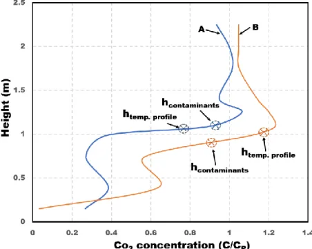
Figure 5. Comparison between the neutral height obtained from contaminant profiles (by visual inspection) and thermal profiles (applying the proposed algorithm). Measurements by Brohus et al. [20]. ... 13
Figure 6. Correlation between calculated and experimental neutral heights. ... 15
Figure 7. Proposed model structure. ... 17
Figure 8. Convective mixing of internal heat gains into the occupied zone (FMO) determination. ... 19
Figure 9. Results of the model simulation for the cases in the database and comparison with measured data. ... 20
Figure 10. Comparison between proposed model, Graça and Linden [33] DV model and measured data. ... 20
Figure 11. Scheme of CC/DV system driving mechanism. ... 24
Figure 12. Experimental average temperature profile of CC/DV and DV systems. ... 28
Figure 13. Schematic representation of three temperature points and temperature gradients. ... 29
Figure 14. Schematic representation of model structure. ... 30
Figure 15. Neutral height position of temperature profiles presented by Rees, et al [63]. ... 31
Figure 16. Convective mixing of heat gains into the occupied zone (FMO) determination. ... 34
Figure 17. Results of the model simulations and comparison with measured data. ... 36
Figure 18. Comparison between proposed model, Rees & Haves CC/DV model, CFD and measured data. ... 37
Figure 19. CC/DV system design chart – low heat gains scenario. ... 40
Figure 20. CC/DV system design chart – high heat gains scenario. ... 40
Figure 22. A- Chimneys and dampers; B- kindergarten NV system scheme; C- interior
view of a kindergarten room with the heated cylinders used in the measurements. .... 51
Figure 23. Locations of the sensors used in the Kindergarten measurements. ... 51
Figure 24. Aerial and interior views of the UL classroom. ... 52
Figure 25. Locations of the sensors used in the UL classroom measurements. ... 53
Figure 26.Kindergarten measurements results: A* and number of plumes impact on indoor air temperature profile. ... 55
Figure 27. Kindergarten measurements results: impact of chimney height on indoor air temperature profile (outdoor air temperature =13.7ºC). ... 56
Figure 28. Kindergarten and UL classroom thermal zones (geometric model). ... 57
Figure 29. Three-node DV model structure implemented on EnergyPlus. ... 58
Figure 30. Inlet CFD simulations: geometry and results. ... 58
Figure 31. Outlet CFD simulations: geometry and results. ... 59
Figure 32. Bulk airflow rate results: measured vs simulated. ... 60
Figure 33. Three-node DV model temperature results comparison. ... 62
Figure 34. Typical office and large DV rooms maximum cooling loads. ... 65
Figure 35. Concert hall: audience and stage. ... 69
Figure 36. Concert hall HVAC system configuration... 69
Figure 37. Locations of the sensors used in the Concert hall measurements. ... 70
Figure 38. Orchestra rehearsal room. ... 70
Figure 39. Locations of the sensors used in the Orchestra rehearsal room measurements. ... 71
Figure 40. Expected vertical temperature profiles produced from different plume types. ... 73
Figure 41. Method used to test plume coalescence. ... 74
Figure 42. Concert hall dynamics: Temperature vertical profile (measurement point nº2). ... 75
Figure 43. Concert hall dynamics: Temperature vertical profile (measurement point nº3). ... 75
Figure 44. Concert hall dynamics: temperature and CO2 concentration vertical profile (measurement point nº2). ... 75
Figure 45. Concert hall dynamics: temperature and CO2 concentration vertical profile (measurement point nº3). ... 76
Figure 46. Concert hall spatial analysis: temperature vertical profiles. ... 76
Figure 47. Concert hall spatial analysis: CO2 concentration vertical profiles. ... 77
Figure 50. Correlation between calculated and experimental neutral heights of all
temperature profiles analyzed. ... 80
Figure 51. Concert hall and Orchestra rehearsal room pollutant removal efficiency. ... 81
Figure 52. Three-node DV model implemented on EnergyPlus. ... 82
Figure 53. Comparison between measurements and EnergyPlus simulations of the Concert hall. ... 84
Figure 54. Comparison between measurements and EnergyPlus simulations of the Orchestra rehearsal room. ... 84
Figure 55. Gulbenkian Concert hall. ... 86
Figure 56. Gulbenkian Concert hall original HVAC system... 87
Figure 57. Concert hall thermal zones. ... 88
Figure 58. Sizing results: Airport weather data, TMY weather file and ASHRAE design days sizing comparison. ... 90
Figure 59. Results: Stalls and balcony UHA sizing - 0.4% Airport weather data. ... 90
Figure 60. Gulbenkian Concert hall CFD model geometry (half room). ... 92
Figure 61. Grid refinement (xx axis) of Gulbenkian Concert hall PHOENICS model. .. 93
Figure 62. Results: Room temperature Classical scenario. ... 94
Figure 63. Results: Room temperature Modern scenario. ... 94
Figure 64. Results: Room velocity Classical scenario. ... 94
Figure 65. Results: Room velocity Modern scenario. ... 95
Figure 66. Results: Classical LB+LN scenario - Room temperature profile. ... 95
Figure 67. Results: Classical LB+LN scenario - Room velocity profile. ... 95
Figure 68. Results: Modern LN+HB scenario - Room temperature profile. ... 96
Figure 69. Results: Modern LN+HB scenario - Room velocity profile. ... 96
Figure 70. Classical HN+LN and Modern HN+LN: high nozzle velocities profile showing fast velocity decay (and thereby limited cooling effect). ... 97
Figure 71: Inside, exterior and courtyard views of the CML Kindergarten. ... 98
Figure 72: Lateral, front and inside views of the German school. ... 99
Figure 73: Typical year of Lisbon weather (outdoor temperature and radiation). ... 99
Figure 74: Kindergartens ventilative cooling systems operation modes (winter and summer). ... 100
Figure 75: CML Kindergarten and German School EnergyPlus model. ... 100
Figure 76: CML Kindergarten results: Operative temperature and CO2 level (winter operation day). ... 102
Figure 77: CML Kindergarten results: Operative temperature and CO2 level (summer operation day). ... 103
Figure 78: CML Kindergarten statistical analysis: operative temperature (EN 15251) and indoor air quality (RECS). ... 103 Figure 79: CML Kindergarten operative temperature adaptive comfort analysis (ASHRAE 55-2010). ... 103 Figure 80: German School results: Operative temperature and CO2 level (winter operation day). ... 104 Figure 81: German School results: Operative temperature and CO2 level (summer operation day). ... 104 Figure 82: German School statistical analysis: operative temperature (EN 15251) and indoor air quality (RECS). ... 104 Figure 83: German School operative temperature adaptive comfort analysis (ASHRAE 55-2010). ... 105
List of tables
Table 1 - Dimensions, internal gains and flow rates of DV test chamber experimental
studies. ... 4
Table 2 - Displacement ventilation nodal models. ... 5
Table 3 - Correspondence between papers and Chapters, referring its application and main topic ... 9
Table 4 - Comparison between concentration and temperature neutral heights for three independent studies. ... 14
Table 5 - Comparison between calculated and experimental neutral heights. ... 15
Table 6 - Validation of proposed model and comparison with Graça & Linden [30] model results. ... 21
Table 7 - Dimensions, internal gains and operating conditions of CC/DV test chamber experimental studies. ... 26
Table 8- Approach used, main focus and typical precision of CC/DV modelling studies. ... 27
Table 9 - Comparison between calculated and experimental neutral heights. ... 33
Table 10 - Validation of the proposed model. ... 35
Table 11 - Comparison of models precision. ... 37
Table 12 - Proposed model and CFD precision comparison. ... 37
Table 12 - Simulated heat gains scenarios. ... 39
Table 13 - CC/DV recommended operating parameters. ... 41
Table 14 - Existing measurement and simulation studies of NV flows. ... 47
Table 15 - Kindergarten building material properties (from []). ... 50
Table 16 - UL classroom material properties. ... 52
Table 17 - Specifications of the measurement equipment used. ... 54
Table 18 - Natural DV measured cases. ... 55
Table 19 - Grid sensibility analysis: discharge coefficient results. ... 59
Table 20 - Comparison between measured and simulated node temperatures: TAF, TOC and TMX. ... 61
Table 21 - Sensitivity analysis: impact of discharge coefficient on three-node DV model simulation results. ... 62
Table 22 - Large rooms studies references. ... 68
Table 23 - Specifications of the measurement equipment used. ... 71
Table 24 - Comparison between calculated and experimental neutral heights. ... 79
Table 26 - Comparison between measured and simulated node temperatures: TAF, TOC and TMX. ... 84 Table 27 – UHA’s sizing criteria. ... 88 Table 28 - Sizing criteria – loads considered in different scenarios. ... 89 Table 29 – CFD simulated scenarios. ... 92 Table 30 - CFD simulation conditions. ... 93 Table 31- CML Kindergarten and German School heat loads scenarios used in
simulation. ... 101 Table 32 - Opening areas summary. ... 102
1. Introduction
In the last decades the rising time that people spend in non-domestic buildings with heating, ventilation and air conditioning systems (HVAC) lead to a significant increase in HVAC related energy consumption in services buildings (up to 50% of the total energy consumed in these buildings [1]). In most non-domestic buildings the HVAC system is predominantly used to provide fresh air and cooling, ideally with the lowest energy consumption possible for a given location and internal load. In air based HVAC systems, the ventilation efficiency and inflow temperature can have a large impact in overall energy efficiency. In this context, the airflow distribution strategy is one of the most relevant decisions in HVAC system design [2,3]. The most commonly used airflow distribution method is mixing ventilation (MV). In MV systems the fresh air is supplied in the upper part of the room, at a temperature below 16ºC [4], mixing the high-level heat loads into the occupied zone promoting uniform air conditions (temperature and pollutants) throughout the whole space. However, the environmental impact of the HVAC systems energy consumption led to the continuous development of energy efficient solutions such as Displacement Ventilation (DV).
DV was initially developed in the 70’s for applications in industrial halls in the Nordic countries. The ability of these systems to concentrate heat and pollutants in the upper portion of the space, where they can be exhausted without affecting the lower portion of the space, led to increased popularity and subsequent use in service buildings (starting in the early 80’s [5]). In an effective DV system fresh air inserted near the floor, is drawn to the heat sources in a low velocity, self-regulating flow that was first studied by Sandberg and Sjoberg (1984) [6] and Skaret (1987) [7]. The inflow air should be supplied with low velocity and an inflow temperature that is 4-6ºC lower than the desired comfort temperature to avoid cold draft discomfort [6,7].The negatively buoyant inflow air spreads over the room floor until it reaches the heat sources where it expands and rises as a thermal plume. In DV, heat loads in higher levels of the room (above the occupied zone) are removed in an ideal way, with no impact in the occupied zone. In DV, whenever the room internal gains occur predominantly in the form of plumes, a noticeable interface occurs between the occupied zone of the room and a mixed hot layer near the ceiling of the room. This temperature and contaminant stratification removes heat and pollutants from the occupied zone with high ventilation efficiency [8,9].
The increased popularity of DV systems created difficulties for designers when sizing and predicting energy consumption of a stratified space that cannot be adequately
modeled with the fully mixed room air approach that is used for overhead air conditioning systems. The need to fine-tune the design of DV systems led to the development of several models with variable complexity. Sandberg and Lindstrom (1987) [10] proposed a mechanical DV design simplified model based on a two-region airflow structure, defining the lower boundary of the mixed upper layer, the neutral height, as the point where the total buoyancy induced plume flow equals the inflow rate [35]. Beyond the neutral height the continuously increasing plume flow is fed by room air, generating a mixed upper layer (this two layer structure is visible in figure 1a). In 1990, Linden et al. [11] developed a similar two-layer model for the more complex case of natural DV, using an experimental setup based on scaled salt-water models. In the salt-water experimental approach, buoyancy variations are generated by varying water salinity level in a container whose walls are impervious to salt, leading to a flow that only displays buoyancy effects from the plume sources (see figure 1a). DV airflows have internal heat sources that are part convective, part radiative and, even in the nearly adiabatic test chambers that are often used in DV system performance assessments, the room air exchanges heat with the room surfaces. The resulting air temperature profiles are smoother than the salinity, CO2 or other non-buoyant pollutant profiles (see figure 1b): the effect of radiative heat transfer and resultant internal surface convective heat transfer is that part of the heat gains are mixed in the occupied zone and not convected upwards. Still, the DV vertical temperature variation profiles exhibit an upper mixed layer where the vertical temperature gradient is small. Controlling the neutral height is a DV system design objective: in most DV application cases there is a coincidence between heat and pollutant sources, resulting in a mixed layer region that contains the indoor pollutants and, therefore, should be kept above the occupants head height (above 1.3m for seated occupants or 1.8m for standing occupants). Increasing the room airflow-rate raises the neutral height by raising the point where the total thermal plume flow matches inflow. In addition to the neutral height, a successful DV system design must be able to control occupied zone and ankle level air temperatures.
Figure 1. Image of DV flow in a scaled salt water mode (left [12]), typical temperature, concentration and salinity profiles (center), and a schematic depiction of a DV flow (right).
Currently, designers of DV systems have three methodologies for system sizing and prediction of energy consumption: simplified design methods [13], simplified models implemented in dynamic thermal simulation tools [14,15,16], and computational fluid dynamics (CFD) models [17,18,19]. With the widespread use of computer simulation, simplified sizing methods are becoming less popular due to their inability to predict whole year energy consumption. CFD is becoming more accessible, and should play an increasing role in HVAC design in the coming decades, but remains, for the moment, too time-consuming to be used in whole year simulation design scenarios. Simplified models implemented in dynamic thermal simulation tools are the most accessible option for design and building energy certification. Furthermore, a successful simplified model can provide insight and understanding of the design parameters that control the room flow field and air temperature.
1.1. Review of existing work
This review of existing work begins with a survey of experimental studies, followed by a brief discussion of the existing simplified models. In the last part, data from one of the experimental studies is used to assess the precision of the two models that are currently implemented in EnergyPlus.
1.1.1.Experimental studies
Existing experimental work on DV systems includes measurements in occupied buildings and test chambers. Model development and validation require complete data sets and controlled boundary conditions that, in the present case, can only be found in studies based on nearly adiabatic, mechanically conditioned test chambers. Table 1 shows the main characteristics of the DV test chamber studies that meet these criteria. Analysis of the table reveals a large range of mechanical ventilation flow rates, internal heat load and heat gain sources (thermal manikins, point sources, computers, etc.). The floor to ceiling height range is limited to typical office heights (2.2-2.8m), with the exception of one case with a large floor to ceiling height [20]. Most test chamber studies include experiments with two or more simultaneous heat sources with different magnitudes that generate asymmetric plumes.
In order to compare temperature profiles from different studies was introduced two commonly used non-dimensional variables (room temperature and height):
θ = T-Tin
Tout-Tin, z * = z
Figure 2 shows a typical test cell and the resulting average non-dimensional temperature profile obtained from the data of the first three studies in table 1.
Figure 2. Typical geometry, heat gains, flow rate and temperature profiles for the test cell studies used to develop the present model.
Table 1 - Dimensions, internal gains and flow rates of DV test chamber experimental studies.
Reference
Test chamber dimensions
Plume type Flow rate
(m3/h) W/m 2 Height (m) Area (m2) H. Brohus, et al. [20]* 2.4 - 4 15 - 48 | vv |
Vv| |
●
| 8 - 27 145 – 395 Yuan, X. [21]* 2.4 19 | Vv | | | 23 183 E. Mundt [22]* 2.6 17 | vv | | 12 87 – 175Ming Xu, et al. [23] 2.2 16 | v | vv | | 6 - 26 162
G. He, et al.[24] 2.3 19 | Vv | | | 5 202
I. Olmedo, et al. [25] 2.7 13 | Vv |
●
| | 57 196Simon J. Rees, et al. [26] 2.8 17 | v | vv | | 6 - 24 68 – 137
Xiufeng Yang, et al. [27] 2.6 11 | v |
●
| 9 40Josephine Lau, et al. [28] 2.7 25 | vv | | 19 -
Lin Tian, et al.[29] 2.6 11 | Vv | | | 23 - v – single plume; vv - multiple symmetric plumes; Vv - multiple asymmetric plumes;
– computer; - person simulator;
●
- point heat source; - radiator;1.1.2. Existing simplified models
This bibliographic review identified three simplified nodal models with different approaches and number of nodes (table 2). There are two models that use a linear temperature variation along the room height. The simpler of these models, proposed by Mundt [30], uses two air nodes: a temperature near the floor surface (ankle level) and an upper node representing the exhaust air temperature. The second of the linear models (Li et al. [31]) is a development of the Mundt approach, using an additional node to characterize air temperature variations near the ceiling (leading to a total of three air nodes). The third model uses a three-node approach (near floor, occupied and mixed layer [32,33]) and predicts the neutral height using the inflow to total plume flow matching approach, discussed above. Temperature variation between the nodes is linear but with different slopes between the nodes (figure 3). This model requires a user-inputted coefficient to characterize the fraction of mixing of the heat gains into the occupied zone.
Table 2 - Displacement ventilation nodal models.
Reference Number of
room air nodes
Temperature gradient Neutral level calculation Mundt (1996) [30] 2 Linear No Li et al. (1992) [31] 3 Linear No
Graça and Linden (2004) [33] 3 Linear, variable
between nodes Yes
1.1.3. Accuracy of existing models
Figure 3 shows two simulations of the test chamber study of Mundt [22] using the two models discussed above that are available in EnergyPlus: Mundt [30] and Graça & Linden [33]. Analysis of the results reveals qualities and limitations in both models, namely:
As expected, both models have good accuracy when predicting the exhaust temperature: it is a direct application of energy conservation.
Both models under predict the ankle level temperature; resulting in significant error in a design parameter that is used to define the inflow temperature and predict thermal comfort. Neither of the models considers mixing of inflow air with
In the Graça and Linden model the results are sensitive to a user-supplied coefficient: the fraction of heat gains mixing into the occupied zone. Further, there is no guidance for the value that the user should use in different gains scenarios. The linear temperature gradient used in the Mundt model does not display the two-layer behavior that is visible in the temperature profiles. This simplification prevents the designer from using the model to fine-tune the inflow rate for improved air quality in the occupied zone.
Figure 3. Comparison between Mundt [30], Graça and Linden [33] DV models and measured data.
The results indicate that the approach used by both models to calculate ankle level temperature, based on adjusting the inflow temperature to incorporate heat exchange with the room floor may be inadequate. This approach may have been more adequate for rooms with inflow through slots, with no diffusion since this simple inflow geometry generates a gravity current of cool inflow air that has limited mixing as it spreads across the room floor. More recent DV systems and experimental facilities use DV flow diffusers that promote mixing with warmer room air, thereby increasing ankle level air temperature and reducing cold draft induced discomfort.
1.1.4. Research questions
The analysis performed in the previous sections resulted in the following research questions that must be addressed in the development of simplified modelling approaches for DV systems:
1. Is the matching of plume flow to inflow approach valid for defining the neutral level in a room with mixed heat sources (convective and radiative)?
2. What is the fraction of heat gain mixing in the occupied zone that best fits the slowly varying temperature profiles found in the experimental data?
3. What is the level of mixing between inflow and room air that best fits the experimental data?
4. How the neutral height position is affected by chilled ceiling temperature in a CC/DV room? Could the proposed DV simplified model be applied to model CC/DV rooms? 5. Are the thermal stratification profiles in occupied buildings with active boundary
conditions similar to the ones measured in (nearly adiabatic) test cell cases? 6. In large DV rooms, how do the radiative heat exchanges with the walls could affect
the expected temperature and contaminants vertical profiles?
7. What is the impact of a thermal chimney in natural DV system performance?
1.2. Publications
The work developed in this thesis resulted in the publication of four papers in international peer-review journals and two refereed conference papers. Further, there are three more journal papers that are currently under review:
Paper I – “Thermal and airflow simulation of the Gulbenkian Great hall” by Nuno M. Mateus and Guilherme Carrilho da Graça published in Proceedings of 13th international conference on building simulation, Chambery, France (2013). Paper II – “Validation of EnergyPlus thermal simulation of a double skin naturally
and mechanically ventilated test cell”, by Nuno M. Mateus, Armando Pinto and Guilherme Carrilho da Graça published in the journal Energy and Buildings, 2014. Paper III – “A validated three-node model for displacement ventilation”, by Nuno M. Mateus and Guilherme Carrilho da Graça published in the journal Building and Environment, 2015.
Paper IV – “Simplified modeling of displacement ventilation systems with chilled ceilings”, by Nuno M. Mateus and Guilherme Carrilho da Graça published in the journal Energy and Buildings, 2015.
Paper V – “Stack driven ventilative cooling for schools in mild climates: analysis of two case studies”, by Nuno M. Mateus and Guilherme Carrilho da Graça, published in Proceedings of 36th AIVC Conference Conference, Madrid, Spain (2015).
Paper VI – “Validation of a lumped RC model for thermal simulation of a double skin natural and mechanical ventilated test cell”, by Marta J.N. Oliveira Panão, Carolina A.P. Santos, Nuno M. Mateus and Guilherme Carrilho da Graça published in the journal Energy and Buildings, 2016.
Paper VII - “The effect of typical buoyant flow elements and heat load combinations on room air temperature profile with displacement ventilation”, by Risto Kosonen, Natalia Lastovets, Panu Mustakallio, Nuno Mateus and Guilherme Carrilho da Graça, submitted to the journal Building and Environment, 2016.
Paper VIII - "Comparison of measured and simulated performance of natural displacement ventilation systems for classrooms”, by Nuno M. Mateus and Guilherme Carrilho da Graça, submitted to the journal Energy and Buildings, 2016.
Paper IX – “Measured performance of a displacement ventilation system in a large concert hall”, by Nuno M. Mateus and Guilherme Carrilho da Graça, submitted to the journal Building and Environment, 2016.
1.3. Outline of thesis
The thesis is organized in seven chapters. Chapter 1 presents a literature review about displacement ventilation concepts, the existing experimental work and the most used modelling approaches. Chapter 2 presents a validated simplified approach for DV that models the room thermal stratification using three air temperature nodes: lower layer (floor level), occupied zone and upper layer. An extension of the proposed model to CC/DV systems is showed and validated on Chapter 3. Chapter 4 presents a set of detailed measurements of buoyancy driven natural DV systems of three classrooms. The measurements were used to analyze the performance of natural DV systems and to validate the three-node DV model (presented on Chapter 2) implemented on the open-source thermal building simulation software EnergyPlus. In Chapter 5, the performance of two DV large rooms was analyzed using a set of detailed measurements. Chapter 6 presents the application of the modeling approaches developed along the thesis in three design projects: two naturally ventilated DV schools and the refurbishment of the Calouste Gulbenkian large concert hall HVAC system. Finally, Chapter 7 presents the conclusions of the work and a discussion of future developments.
Table 3 presents the relation between the papers that resulted from this thesis and the chapters.
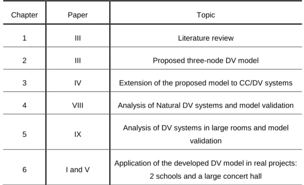
Table 3 - Correspondence between papers and Chapters, referring its application and main topic
Chapter Paper Topic
1 III Literature review
2 III Proposed three-node DV model
3 IV Extension of the proposed model to CC/DV systems
4 VIII Analysis of Natural DV systems and model validation
5 IX Analysis of DV systems in large rooms and model validation
6 I and V Application of the developed DV model in real projects: 2 schools and a large concert hall
2. A validated three-node model for displacement
ventilation
This chapter presents a simplified model for DV that approximates the room thermal stratification using three air temperature nodes: lower layer (floor level), occupied zone and upper layer. The proposed model is a development of a model that is currently available in the thermal simulation tool EnergyPlus. The proposed developments increase modeling accuracy and robustness by minimizing the need for user supplied coefficients. The following sections presents an analysis of the applicability of plume flow theory as a criterion to establish the neutral level, followed by a presentation of the model equations. Finally, in section 2.3, is presented the model validation using results from several independent experimental campaigns.
2.1. Prediction of neutral height
In concentration profiles, such as the ones shown in figure 5, the location of the neutral height can be defined by visual inspection. In contrast, in the temperature profiles found in DV rooms, this location is much more difficult to identify (Huijuan Xing et al. (2002) [34]). This section investigates whether the temperature gradient found in DV rooms with approximately adiabatic boundary conditions displays a neutral height that can be predicted using the plume flow to inflow matching principle. For this purpose, i begin by developing and validating a quantitative method to locate the neutral height in temperature gradients. Then, i proceed to use the method to obtain the neutral height for a set of experimental cases where only temperature profiles are available (the most common scenario). Finally, this dataset is used to check the applicability of the plume flow matching principle to rooms with mixed heat sources and heat transfer in the envelope.
To model the vertical variation of the total flow from a point plume the solution proposed by Morton et al. (1956) [35] was used:
F = 65 𝛼43 √9 10 3 π23 √g β W ρ Cp h 5 3 (2)
This expression includes two coefficients, 𝛽 and 𝜌, that are temperature dependent and were determined using the average values for the experimental cases that are used to test the model (resulting in, 𝛽= 0.0034 and 𝜌 = 1.14kg/m3). The other constant in this expression,𝛼, accounts for ambient fluid entrainment (Morton et al. (1956) [35], 𝛼 = 0.13).
Rearranging equation 2 to isolate the neutral height, h, for a given room inflow F, and point buoyancy source W, was obtained:
h = 23.95 √F3 W
5
(3)
When there are n non-coalescing plumes with equal strength the neutral height is given by:
h = 23.95 √5 W nF33 (4)
Equation 2 was developed for plumes generated by point sources of convective heat. Yet, the heat gains found in real building are generated in the surface or a volume such as an occupant or a computer monitor (for both cases most experimental studies propose a 50% split between convective and radiative heat gains). To apply the point plume expression to these geometries a virtual origin must be defined for each heat source [36,37,38]. The virtual origin will be positioned at a height z0 below the top of the heat source and can be calculated using two different approaches. In the minimum approach the spreading angle of the plume is 25º and the virtual origin is located approximately one third of the heat source characteristic diameter above the bottom of the heat source. In the maximum approach the point source is located in a point so that the border of plume above that point passes through the top edge of the real source [39]. In the present case, it was proposed to use the minimum approach to correct for the point plume height when using real sources (a conservative approach).
In cases where there are several buoyancy sources there is a need to check for two factors: thermal plume coalescence and relative strength of the buoyancy sources. Coalescence is a factor because the total plume flow rate of coalesced plumes increases less with height due to a smaller entrainment perimeter (compared to two isolated plumes). For this reason, the neutral height will rise if plumes coalesce before the mixed upper layer. Figure 4 shows the method used to check for plume coalescence (based on the minimum approach described above). In the example shown in the figure there is no coalescence effect since: Xplume1+Xplume2 > X12 is larger than h12 (the neutral height calculated using expression 4, with n=2). Expression 4 is valid for n plumes of equal strength. For n plumes of unequal strength was proposed an approximate application of this expression by considering n plumes of equal strength. Still, because the proposed method relies on an identifiable temperature transition, the experimental cases used below have, in each case, a maximum range of asymmetry in plume strength of two to one.
Figure 4. Geometric method to test plume coalescence.
2.1.1 Methodology for predicting the neutral height from temperature profiles
To develop the methodology i will use three independent experimental studies with simultaneous measurement of CO2 concentration and temperature (shown in table 3). Analysis of the temperature profile shown in figure 3can provide hints for a successful quantitative methodology to locate the neutral height: the rate of temperature increase between the floor and the lower part of the mixed layer is markedly higher than in the rest of the room height. The proposed method locates the point in the region of this gradient transition that matches the neutral height obtained from concentration gradients. I start by defining the average normalized temperature gradient along the total room height (NTG):
NTG =Tzceiling-Tzfloor
Zceiling-Zfloor (5)
Next, all experimental temperature profiles are discretized using one hundred, equally spaced points (along z, from floor to ceiling) and a rolling average smoothing with a ± 0.1m vertical averaging interval is applied to avoid false results due to local inflections in the experimental profiles. Starting from the floor, the method uses a forward marching logic check to identify the first point with a local gradient, defined using points z+1 and z, that is larger than NTG by a factor that will be calculated using the three cases where both profiles are available:
(1+CNH) ×
Tztotal-Tz0 Ztotal-Z0 >
Tz+1-Tz
To find the value of the coefficient (CNH) that result in the best agreement between
temperature and pollutant profile based neutral heights the method was applied to the profiles measured in three independent experimental studies shown in table 3. The best fit was obtained when: CNH = 0.3. Figure 5 shows the results of applying the method to
one of the three studies used (Brohus et al [20]).
Figure 5. Comparison between the neutral height obtained from contaminant profiles (by visual inspection) and thermal profiles (applying the proposed algorithm). Measurements by Brohus et al. [20].
To quantify the differences between the neutral heights predicted by the two methods the following error indicators were used:
Bias (m) = htemp. profile- hcomtaminants (7) Error (%) = 100% × |htemp. profile- hcomtaminants
Table 4 - Comparison between concentration and temperature neutral heights for three independent studies.
Reference htemp. profile hcontaminants Bias (m) Error (%)
Brohus et al. [20] 1.04 1.06 -0.02 1.7 1.01 0.91 0.10 9.8 Bouzinaoui et al. [40] 3.98 3.83 0.15 3.8 Trzeciakiewicz, et al. [41] 0.83 0.91 -0.08 9.6 Average indicators 0.04 6.2
The results presented in table 3 confirm the validity of the proposed method: the bias is negligible (4cm) and the maximum error is less than 10%.
2.1.2 Validation of neutral height prediction
The method developed in the previous subsection can be used to evaluate the precision of expressions 4 and 5 using a larger set of experimentally measured temperature profiles, shown in table 1, including different heat gains densities, airflow magnitudes and type of heat gain. Still, not all studies presented in table 1 can be used to validate the model since, in some cases, not all the test cell dimensions, airflow rate, temperature and heat gain information is available. Further, the heat gains must be static and not unrealistically small: Cases with internal heat gains of less than 7.5 W/m2 should be avoided since typical office buildings have at least 20W/m2. Cases with very small heat gains display large effects of heat loses in the envelope that, in some cases, can exceed 10% of the total heat gains [42]. Application of these rules resulted in three selected studies that will be used to validate the model presented in this paper: Brohus et al. [20], Yuan [21], Mundt [22] (the first three cases in table 1, signaled with a “*”).
The results shown in table 4 and figure 6 confirm the applicability of expressions 4 and 5 to predict the neutral height. The average error obtained is 14%, and the correlation coefficient, R2, is 0.69.
Figure 6. Correlation between calculated and experimental neutral heights.
Table 5 - Comparison between calculated and experimental neutral heights.
Reference hcalculated (m) hmeasured (m) Bias (m) Error (%) Brohus et al. [20] 0.82 1.04 0.22 21.0 0.82 1.01 0.19 19.1 1.14 1.45 0.30 20.9 1.16 1.29 0.12 9.5 1.14 1.08 -0.06 5.8 1.44 1.56 0.11 7.4 1.80 1.76 -0.04 2.4 Yuan [21] 1.13 1.16 0.04 3.3 Mundt [22] 0.90 0.71 -0.18 25.7 1.08 0.82 -0.26 32.0 1.24 1.37 0.13 9.2 Average indicators 0.18 14.2
2.2. A simplified three node DV model
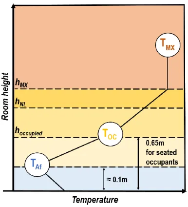
The proposed model extends the perfectly mixed room air single node approach to three nodes located along the room height (shown in figure 7). The model considers fully mixed air in each node and a linear air temperature variation between nodes. The three model nodes represent three distinct room regions:
The floor level air temperature node (TAf) characterizes the temperature of the air that is entrained by the plumes into the occupied zone. This point is located at 0.1m height.
The occupied zone air temperature node (TOC) is located in the center of the occupied zone (0.65m for seated occupants and 0.9m for standing occupants). The mixed layer air temperature node (TMX) characterizes the exhaust/mixed
layer temperature and represents a region that begins above the neutral height and ends at the ceiling. In the model, this region is isothermal.
All plumes are modeled as point sources of buoyancy. The floor level temperature is obtained by imposing energy conservation to the balance between the heat that is exchanged with the floor, convected to the occupied zone (with the flow rate F), and the portion of air that is mixed with the air of the occupied zone. Measurements by Fatemi et al. [43] show that, at a distance of 3.5m from a DV corner diffuser there is as an entrainment generated accumulated flow rate increase of approximately 60% (IM = 0.6 in
equation 9). This mixing between inflow and room air is not modeled in any of the three existing models and will be introduced in the improved model. Finally, the neutral height is predicted using expression 3 or 4 (for single or multiple plumes). The energy conservation equations for the three model nodes are the following:
ρ.Cp.F.Tin + IM.ρ.Cp.F.TOC + Af.hf.(Tf - TAf) = (1+IM).ρ.Cp.F.TAf (9) (1+IM).ρ.Cp.F.TAf - IM. ρ.Cp.F.TOC +FMO .FGC.G + Awl.hwl.(Twl - TOC) = ρ.Cp.F.TOC (10) ρ.Cp.F.TOC + FGC.G.(1 - FMO) + Ac.hc. (Tc - TMX) + Awu.hwu.(Twu - TMX) =ρ.Cp.F.TMX (11) The parameter FMO characterizes the fraction of the convective heat gains that is mixed
into the occupied zone, and, therefore, not convected directly to the mixed layer (0< FMO
<1). This lower level mixing does not occur in an ideal displacement system (FMO =0). As
discussed above in the existing three-node model [32] the value of this parameter was not known, yet, as shown in figure 3, its effects on the results are relevant. The database that will be used to validate the model in the next section will be used to obtain the best-fit value for FMO.
Heat transfer from internal surfaces is evaluated using convection coefficients developed for DV heat transfer (Novoselac et al. (2006) [44]) and the air temperature of the room node that is in direct contact with the surface: the floor surface is coupled to TAf, the ceiling is coupled to TMX and the lateral surfaces are coupled to Toc or TMX (depending on their vertical location). For lateral surfaces that are in contact with the occupied zone and
mixed layer an area weighted room air temperature is used. Radiation heat exchange between surfaces is evaluated using exact view factors that are available for rectangular cavities [45]. The room surface energy conservation equations are the following:
hc(Tc - TMX) + hrc(Tc -Tf Af +TwlA Awl + Twu Awu t - Ac ) = FGR G/At (12) hf (Tf - TAf) + hrf(Tf -Tc Ac+ TwlA Awl + Twu Awu t - Af ) = FGR G/At (13) hwl(Twl- TOC ) + hrwl(Twl -Tc Ac + TAf Af+ Twu Awu t - Awl ) = FGR G/At (14) hwu(Twu - TMX) + hrwu(Twu -Tc Ac +TAf Af +Twl Awl t - Awu ) = FGR G/At (15) This seven equation system (equations 9-15) is nonlinear due to the temperature difference dependent convective heat transfer correlations. As in other models implemented in EnergyPlus, coupling between the energy balance equations (9-15) and the convection correlations is indirect: air and surface temperatures from the previous time step are used to calculate heat transfer coefficients that are used in the following time step. This coupling approximation has no effect on the steady state validation cases presented below: the solutions algorithm ran until the solution stabilized (typically in 10 iterations).
2.3. Model validation
This section presents an assessment of model precision based on experimental data from the first three studies shown in table 1 (for a total of nine different cases). In addition, this database will be used to define the height of the mixed layer node (TMX) as a function of neutral height as well as finding the best-fit value for the parameter that characterizes heat gain mixing (FMO). The model predictions will be evaluated using the following
average error indicators:
The average norm of the error: Avg. Dif. (K) = ∑9i=1|Sim.i-Meas.i|
9 (16)
The average bias: Avg. Bias (K) = ∑9i=1Sim.i-Meas.i
9 (17)
The average percentage error: Avg. Error (%) =100%9 × ∑ |Meas.Sim.i-Meas.i Max.-Meas.Min.|
9
i=1 (18)
The first application of the experimental database is to define the height of the mixed air node (TMX). As shown in section 2.1, in all temperature profiles analyzed, the neutral height is lower than the bottom of the boundary of the room region where the vertical temperature gradient tends to zero. The upper mixed layer model node (TMX) should be
positioned in the lower edge of this nearly zero gradient region. Analysis of the portion of the nine profiles that is above the neutral height revealed that the zero gradient region begins at the height:
hTMX=h+ hceiling-h
3 (19)
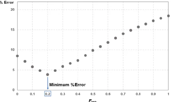
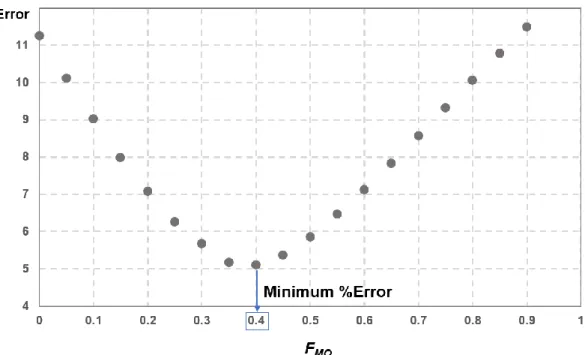
The second application of the experimental database and error indicators is to obtain the best-fit value for the parameter that models convective mixing of internal heat gains into the occupied zone (FMO). For this purpose, model runs with FMO varying between zero
and one were performed. The results of these simulations show that the best-fit value is 0.4 (figure 8). This value is identical to the value found by the same authors when comparing the model predictions with CFD simulations of the large concert hall [46].
Figure 8. Convective mixing of internal heat gains into the occupied zone (FMO) determination.
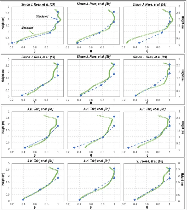
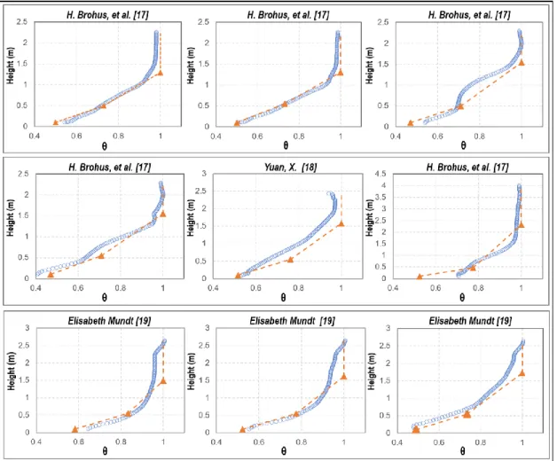
Figure 9 shows the results of the model simulation of the nine cases in the database. In light of the model simplicity the results are encouraging: general agreement is good in all nodes. The discrepancies found in some cases were expectable given the large amount of model simplifications used and uncertainties in the experimental boundary conditions (in most experimental studies the boundaries can be best described as “nearly adiabatic” [26]). Figure 10 shows a comparison between the existing and improved model. The improvements are clear, particularly in the floor level and occupied zone temperature predictions.
Figure 9. Results of the model simulation for the cases in the database and comparison with measured data.
Figure 10. Comparison betweenproposed model, Graça and Linden [33] DV model and measured data.
Table 5 shows the values of the average error indicators for the nine temperature profiles. The overall average simulation error of 5%. The node with the largest average
error is Taf (6%) with a bias towards under prediction. The average temperature error is 0.3K in a dataset that has an average temperature difference between inlet and outlet of 5K. Table 5 also includes the error indicators for the existing model: the improvement is clearly visible in the overall reduction of 17% in model error.
Table 6 - Validation of proposed model and comparison with Graça & Linden [33] model results.
Node
Dif. (K) Bias (K) Error (%)
Proposed model Graça& Linden model Proposed model Graça& Linden model Proposed model Graça& Linden model Taf 0.3 1.5 -0.2 -1.5 6.2 31.4 TOC 0.2 1.7 0.1 -1.7 3.7 28.6 TMX 0.3 0.4 0.1 -0.4 5.3 5.6 Average 0.3 1.2 0.0 -1.2 5.1 21.9 Model limitations
In light of the approximations used in the model, it is expectable that the modeling precision will be greatly reduced in the following cases:
Internal gains split into several highly asymmetric plumes: these cases generate a stratification profile with several neutral levels that is not captured by the current model.
Internal heat gains that are predominantly radiative: in these cases convective heat transfer in the room surfaces heated by the radiative gains can compete with the convective heat gains in the occupied zone, creating a more linear temperature gradient with no identifiable neutral level.
Spaces that are dominated by facade heat gains: ideally the total heat exchange with the building envelope must be one order of magnitude lower than the total occupied zone internal gains (as in the test chamber studies that were used to validate the model). This topic will be analyzed in Chapter 4.
When high-level lighting loads, currently not explicitly included in the model, are comparable to the occupied zone heat gains.
Rooms with chilled ceilings or chilled floors.
This last limitation is not due to the physics of the model since heat transfer from a chilled ceiling or floor is considered in the model equations. Still, additional research on this
topic to investigate the chilled ceiling capability to disrupt the stratification and the effects of a chilled floor on ankle level temperature will be addressed in Chapter 3.
2.4. Conclusions
A simplified three-node model for prediction of temperature gradient and neutral level location in DV rooms was successfully developed and validated using three independent experimental studies. In addition, a methodology for locating the neutral height in temperature profiles was developed and a verification of the applicability of Taylor’s plume flow equation to predict the neutral level in DV rooms was performed. The proposed model provides significantly improved precision when compared to existing DV nodal models, in particular in the floor level and occupied zone temperatures.
Tests of the Taylor point plume flow equation using a database composed of eleven cases from three independent studies showed that, when applying the total plume flow to inflow matching approach, using Taylor’s expression to model plumes generated by real heat sources, the average error in neutral level prediction is 14%. The same database was used to validate the temperature predictions of the model, revealing an average error in the three room node temperatures of 0.3K (5%).
The proposed model is easy to use when implemented in a whole year building thermal simulation tool. Model inputs are limited to the height, number and magnitude of the heat sources in the occupied region. The capability of the model to predict the effect of inflow rate on the location of the neutral height allows for straightforward fine-tuning of DV designs.
3. Simplified modeling of Displacement Ventilation
systems with Chilled Ceilings
In the HVAC design community DV systems are known to be an effective air distribution strategy for office buildings due to its potential to reduce room air velocities, ventilation induced noise and HVAC energy consumption [47]. In spite of these well-established qualities these systems do not have widespread use due to poor heating performance and limited space cooling capability (25-35W/m2 [48,49,50]). Continuous improvement in building envelope insulation has greatly decreased the need for space heating. Still, in many office buildings conventional DV cannot remove the maximum cooling load that often exceeds 50W/m2. To overcome this cooling limitation the HVAC design and research community has developed two DV system variants: under floor air distribution (UFAD [51]) and the combination of DV with chilled ceiling systems (CC/DV [52,53]). In UFAD systems air is inserted into the room from an under floor plenum using swirl diffusers that induce more mixing than standard DV diffusers, allowing for a higher differential between inflow and room air temperature difference (10ºC) and, consequently, higher cooling capacity. In the CC/DV approach, shown in Figure 11, DV inflow air removes the latent loads and a portion of the sensible load, while the CC system removes the remaining sensible load (mostly by radiative heat transfer). With this combined approach the cooling capacity can reach 100 W/m2 [54,55] while maintaining the use of standard low velocity DV diffusers. In a successful CC/DV system, the CC is able to add cooling power without compromising the stratified DV flow.
Design of stratified ventilation systems is more complex than conventional overhead mixing systems since the perfectly mixed room air approximation cannot be used to predict internal conditions. In fact, the main goal in DV modeling is to predict the vertical temperature gradient in the room and also manage the position of the lower boundary of the upper layer of room air where indoor pollutants are concentrated. These seemingly simple tasks are difficult as many flow and room geometry features contribute to the stratification: room height, airflow rate and temperature, type, location and strength of the buoyancy sources. Accurate prediction of the vertical temperature gradient is key for fine tuning of system design and sizing as well as accurate predictions of energy consumption and thermal comfort. The inclusion of a CC system increases the complexity of the design by adding the need to use its cooling power without compromising the stratified environment of the DV system. An excessively low CC surface temperature can destroy the stratification and even create condensation in the
![Table 6 - Validation of proposed model and comparison with Graça & Linden [33] model results](https://thumb-eu.123doks.com/thumbv2/123dok_br/15497584.1044013/44.892.152.747.252.480/table-validation-proposed-model-comparison-graça-linden-results.webp)
![Figure 12. Experimental average temperature profile of CC/DV and DV [71] systems.](https://thumb-eu.123doks.com/thumbv2/123dok_br/15497584.1044013/51.892.140.754.105.483/figure-experimental-average-temperature-profile-cc-dv-systems.webp)
![Figure 15. Neutral height position of temperature profiles presented by Rees, et al [63]](https://thumb-eu.123doks.com/thumbv2/123dok_br/15497584.1044013/54.892.176.718.363.658/figure-neutral-height-position-temperature-profiles-presented-rees.webp)