Numerical analysis of cross-ventilation in generic isolated building configurations

(1)

UNIVERSIDADE DE LISBOA

FACULDADE DE CIÊNCIAS

DEPARTAMENTO DE ENGENHARIA GEOGRÁFICA, GEOFÍSICA E ENERGIA

Numerical analysis of cross-ventilation in generic isolated

building configurations

João Maria Bravo Vieira Dias

Dissertação de Mestrado Integrado em Engenharia da Energia e do Ambiente

(2)

(3)

UNIVERSIDADE DE LISBOA

FACULDADE DE CIÊNCIAS

DEPARTAMENTO DE ENGENHARIA GEOGRÁFICA, GEOFÍSICA E ENERGIA

Numerical analysis of cross-ventilation in generic

isolated building configurations

João Maria Bravo Vieira Dias

Dissertação de Mestrado Integrado em Engenharia da Energia e do Ambiente

Trabalho realizado sob a supervisão de

Prof. Dr. Ir. Bert Blocken (TU/e)

Prof. Dr. Ir. Guilherme Carrilho da Graça (FCUL)

(4)

(5)

Abstract

This thesis presents a numerical analysis of cross-ventilation in generic isolated building configurations. This study focuses on understanding how cross-ventilation is affected by changing the length of the building, the number of partitions and the position of the partition opening for a generic building configuration. Firstly the depth of the building was changed (2.5, 5 and 10 times the building height) and it was found that the volume flow rate through the inlet opening was constant, the air exchange rate decreased proportionally with the building depth, the CO2

concentration and the mean age of air increased with the building depth. The air exchange efficiency was higher in the deepest building and, for this particular case, cross-ventilation was efficient for a building depth ten times the building height. Secondly three different buildings with a partition wall and a door opening were tested for two different building depths. It was concluded that the geometries where the door opening was located close to the side wall (not in front of the inlet/outlet openings) outperformed the other different geometries (including the cases without partition) in terms of mean age of air, CO2 concentration, volume flow rate, air

exchange rate and air exchange efficiency.

(6)

Resumo

Esta dissertação apresenta uma análise numérica de ventilação cruzada em diferentes configurações de um edifício genérico e isolado. Este estudo foca-se em perceber como é que a ventilação cruzada é afectada pela alteração do comprimento do edifício, pelo número de partições e pela posição da abertura entre diferentes partições. Primeiramente, a profundidade do edifício foi alterada (para 2.5, 5 e 10 vezes a altura do edifício) e descobriu-se que o caudal de entrada na abertura a montante do edifício é constante, a renovação de ar decresceu proporcionalmente com o aumento do comprimento do edifício, enquanto a concentração de CO2 e a idade média do ar aumentaram com o aumento do comprimento do edifício. A eficiência

de renovação do ar foi mais elevada nos edifícios mais compridos e, para este caso em particular, a ventilação cruzada foi eficaz num edifício com o comprimento igual a dez vezes a sua altura. Em segundo lugar acrescentou-se à geometria anterior uma parede com uma abertura equiavalente a uma porta, em que ambas mudam de posição, e que divide o espaço interior em dois. Três geometrias foram testadas para dois comprimentos do edifício (padrão e 2.5 vezes a altura do edifício). Foi possível concluir que nos edifícios em que a abertura entre as duas divisões está colocada perto da parede lateral do edifício (não estando na direcção da abertura de entrada/saída do ar exterior) melhores resultados foram obtidos quando comparados com as outras geometrias (incluindo os casos sem partição) em relação à idade média do ar, concentração de CO2, caudal de entrada de ar, renovação de ar e eficiência de renovação de ar.

(7)

Acknowledgments

I would like to thank my home institution coordinator, Professor Guilherme Carrilho da Graça, who gave me the opportunity to study abroad. I would not have had the privilege to work with a great team of professionals in Computational Fluid Dynamics, headed by Professor Bert Blocken, in the Eindhoven University of Technology (TU/e) if it had not been for him.

I would like to express my deepest appreciation to the Building Physics and Services (BPS) department for receiving and helping me during my stay in Eindhoven. I express my genuine gratitude to Professor Bert Blocken for receiving me in his research group and guiding me throughout this thesis. I also want to show my gratefulness to Twan van Hooff and Katarina Kosutova for their availability, for all the sapient advices and critics received along the concretization process.

I would like to thank Pedro who helped during the realization of this work and shared the whole Eindhoven experience with me. I also would like to thank my friends and colleagues that were part of this journey.

At last I want to thank my family for all the support and motivation during my stay in Eindhoven and my girlfriend, Sara, for all the patience, advices and encouragement.

(8)

List of figures

Figure 1 Single-sided ventilation (Awbi 2003). ... 4

Figure 2 Cross-ventilation (Awbi 2003). ... 5

Figure 3 Changes in the minimum ventilation rates in the USA (Awbi 2003). ... 7

Figure 4 Different types of control volumes or cells (Ansys 2009). ... 15

Figure 5 Opening configurations considered for studying the effect of wall porosity and opening location on ventilation flow rate (Karava et al. 2011). ... 19

Figure 6 Velocity and Turbulence intensity profiles considered for the PIV measurements (Karava 2008). ... 20

Figure 7 Profile of x velocity component on the center-line directly between the inlet and outlet openings (PIV measurements on a horizontal and vertical plane and single-point hot-film data) (Karava et al. 2011). ... 21

Figure 8 Cross-sectional view of mean velocity vector field on a vertical mid-plane with 10% wall porosity (Karava et al. 2011). ... 22

Figure 9 Schematic diagram of experimental setup (left). Geometry of internal partition wall (right). ... 23

Figure 10 Building model and measurement plane used for PIV measurements by Karava et al. (2011). ... 25

Figure 11 Schematic view of the four different building configurations (Bangalee et al. 2013). ... 26

Figure 12 Schematic diagram of the full-scale building with a vertical partition inside (Chu & Chiang 2013). ... 26

Figure 13 Computational grid (443,580): (a) Perspective of the inlet, bottom, side and building of the computational domain; (a) Perspective view of the building and ground surface grid... 28

Figure 14 Inlet profiles of mean wind speed (U), turbulent kinetic energy (k) and turbulence dissipation rate (ε). ... 29

Figure 15 Scaled residuals monitored during 10,000 iterations. ... 30

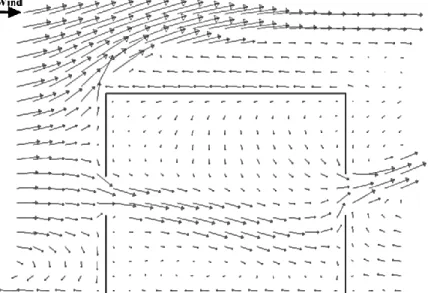
Figure 16 Comparison of the velocity vector fields on the vertical mid-plane between: (a) the PIV measurements and (b) the CFD simulation on the vertical mid-plane scaled by a factor of 8. ... 31

Figure 17 Comparison of the velocity vector fields on the horizontal mid-plane (h = 0.04 m) between (a) the PIV measurements and (b) the CFD simulation scaled by a factor of 8. ... 32

Figure 18 Close up view of the velocity vector field after the outlet opening in the PIV measurements. ... 32

Figure 19 Comparison between the PIV measurements and the CFD simulations for the streamwise wind speed normalized by the reference velocity, on a center-line passing between the two openings (h = 0.04 m). ... 33

Figure 20 Comparison between the PIV measurements and the different CFD simulations for the streamwise wind speed normalized by the reference velocity, on a center-line passing between the two openings (h = 0.04 m)... 34

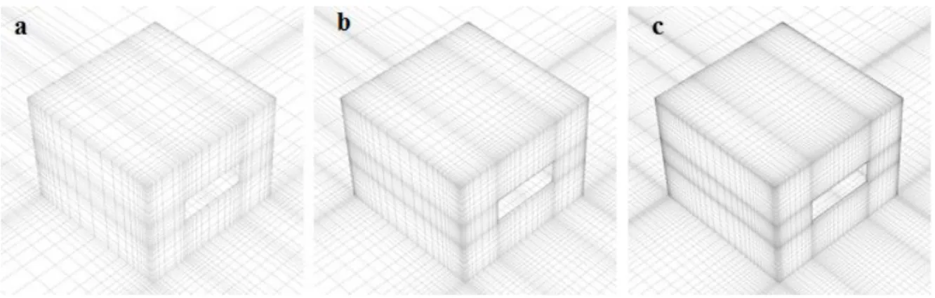
Figure 21 Perspective view of the building and ground surface grid: (a) Coarser grid with 153,303 cells; (b) Standard grid with 443,580 cells; (c) Finer grid with 1,216,068 cells ... 34

Figure 22 Comparison of the streamwise wind speed normalized by the reference velocity, on a center-line passing between the two openings (h = 0.04 m) for the three different grids. ... 35

(11)

Figure 23 Perspective of the inlet, bottom, side and building of the computational domain: (a) Upstream length of the domain equal to 5H; (b) Standard grid with upstream length of the domain equal to 3H. ... 35 Figure 24 Comparison of the streamwise wind speed normalized by the reference velocity, on a center-line passing between the two openings (h = 0.04 m) for the standard grid (3H) and the 5H grid. ... 36 Figure 25 Scaled inlet profiles of mean wind speed (U), turbulent kinetic energy (k) and turbulence dissipation rate (ε). ... 41 Figure 26 Velocity vector field on the vertical mid-plane of the standard building depth. ... 43 Figure 27 Velocity vector field on the horizontal mid-plane (h = 1.2 m) of the standard building depth. ... 43 Figure 28 CO2 concentration on the standard building depth: (a) Vertical center mid-plane; (b)

Vertical left-plane (0.75 m to the left of the mid-plane); (c) Vertical right-plane (0.75 m to the right of the mid-plane). ... 44 Figure 29 CO2 concentration on the standard building depth: (a) Horizontal 0.1 m plane; (b)

Horizontal 1.1 m plane; (c) Horizontal mid-plane (1.2 m); (d) Horizontal 1.7 m plane. ... 45 Figure 30 Velocity vector field on the vertical mid-plane of the 2.5 H building depth. ... 46 Figure 31 Velocity vector field on the horizontal mid-plane (h = 1.2 m) of the 2.5 H building depth. ... 47 Figure 32 CO2 concentration on the 2.5 H building depth: (a) Vertical center mid-plane; (b) Vertical

left-plane (0.75 m to the left of the mid-plane); (c) Vertical right-plane (0.75 m to the right of the mid-plane); (d) Horizontal 0.1 m plane; (e) Horizontal 1.1 m plane; (f) Horizontal mid-plane (1.2 m); (g) Horizontal 1.7 m plane. ... 48 Figure 33 Velocity vector field on the vertical mid-plane of the 5 H building depth. ... 49 Figure 34 Velocity vector field on the horizontal mid-plane (h = 1.2 m) of the 5 H building depth. 49 Figure 35 CO2 concentration on the 5 H building depth: (a) Vertical center mid-plane; (b) Vertical

left-plane (0.75 m to the left of the mid-plane); (c) Vertical right-plane (0.75 m to the right of the mid-plane); (d) Horizontal 0.1 m plane; (e) Horizontal 1.1 m plane; (f) Horizontal mid-plane (1.2 m); (g) Horizontal 1.7 m plane. ... 51 Figure 36 Velocity vector field on the vertical mid-plane of the 10 H building depth. ... 52 Figure 37 Velocity vector field on the horizontal mid-plane (h = 1.2 m) of the 10 H building depth. ... 52 Figure 38 CO2 concentration on the 10 H building depth: (a) Vertical center mid-plane; (b) Vertical

left-plane (0.75 m to the left of the mid-plane); (c) Vertical right-plane (0.75 m to the right of the mid-plane); (d) Horizontal 0.1 m plane; (e) Horizontal 1.1 m plane; (f) Horizontal mid-plane (1.2 m); (g) Horizontal 1.7 m plane. ... 54 Figure 39 Air exchange rate and average CO2 concentration for the four different depths... 56

Figure 40 Local maximum and volume average CO2 concentration for the four different depths. 56 Figure 41 Blueprint at mid-height for the three different configurations. ... 57 Figure 42 Velocity vector field on the vertical mid-plane of the standard building depth with a door in the center of the building. ... 58

(12)

Figure 43 Velocity vector field on the horizontal mid-plane (h = 1.2 m) of the standard building depth with a door in the center of the building. ... 59 Figure 44 CO2 concentration on the standard building depth with a door in the center of the

building: (a) Vertical center mid-plane; (b) Vertical left-plane (0.75 m to the left of the mid-plane); (c) Vertical right-plane (0.75 m to the right of the mid-plane)... 60 Figure 45 CO2 concentration on the standard building depth with a door in the center of the

building: (a) Horizontal 0.1 m plane; (b) Horizontal 1.1 m plane; (c) Horizontal mid-plane (1.2 m); (d) Horizontal 1.7 m plane. ... 61 Figure 46 Velocity vector field on the vertical mid-plane of the standard building depth with a door near the inlet of the building. ... 62 Figure 47 Velocity vector field on the horizontal mid-plane (h = 1.2 m) of the standard building depth with a door near the inlet of the building. ... 63 Figure 48 CO2 concentration on the standard building depth with a door near the inlet of the

building: (a) Vertical center mid-plane; (b) Vertical left-plane (0.75 m to the left of the mid-plane); (c) Vertical right-plane (0.75 m to the right of the mid-plane)... 64 Figure 49 CO2 concentration on the standard building depth with a door near the inlet of the

building: (a) Horizontal 0.1 m plane; (b) Horizontal 1.1 m plane; (c) Horizontal mid-plane (1.2 m); (d) Horizontal 1.7 m plane. ... 65 Figure 50 Velocity vector field on the vertical mid-plane of the standard building depth with a door near the left side wall... 66 Figure 51 Velocity vector field on the horizontal mid-plane (h = 1.2 m) of the standard building depth with a door near the inlet of the building. ... 67 Figure 52 CO2 concentration on the standard building depth with a door near the left side wall: (a)

Vertical center mid-plane; (b) Vertical left-plane (0.75 m to the left of the mid-plane); (c) Vertical right-plane (0.75 m to the right of the mid-plane). ... 68 Figure 53 CO2 concentration on the standard building depth with a door near the left side wall: (a)

Horizontal 0.1 m plane; (b) Horizontal 1.1 m plane; (c) Horizontal mid-plane (1.2 m); (d) Horizontal 1.7 m plane. ... 69 Figure 54 Velocity vector field on the vertical mid-plane of the 2.5 H building depth with a door in the center of the building. ... 70 Figure 55 Velocity vector field on the horizontal mid-plane (h = 1.2 m) of the 2.5 H building depth with a door in the center of the building. ... 71 Figure 56 CO2 concentration on the 2.5 H building depth with a door in the center of the building:

(a) Vertical center mid-plane; (b) Vertical left-plane (0.75 m to the left of the mid-plane); (c) Vertical right-plane (0.75 m to the right of the mid-plane); (d) Horizontal 0.1 m plane; (e)

Horizontal 1.1 m plane; (f) Horizontal mid-plane (1.2 m); (g) Horizontal 1.7 m plane. ... 72 Figure 57 Velocity vector field on the vertical mid-plane of the 2.5 H building depth with a door near the inlet of the building. ... 73 Figure 58 Velocity vector field on the horizontal mid-plane (h = 1.2 m) of the 2.5 H building depth with a door near the inlet of the building. ... 74 Figure 59 CO2 concentration on the 2.5 H building depth with a door near the inlet of the building:

(13)

Vertical right-plane (0.75 m to the right of the mid-plane); (d) Horizontal 0.1 m plane; (e)

Horizontal 1.1 m plane; (f) Horizontal mid-plane (1.2 m); (g) Horizontal 1.7 m plane. ... 75 Figure 60 Velocity vector field on the vertical mid-plane of the 2.5 H building depth with a door near the left side wall... 76 Figure 61 Velocity vector field on the horizontal mid-plane (h = 1.2 m) of the 2.5 H building depth with a door near the inlet of the building. ... 77 Figure 62 CO2 concentration on the 2.5 H building depth with a door near the left side wall: (a)

Vertical center mid-plane; (b) Vertical left-plane (0.75 m to the left of the mid-plane); (c) Vertical right-plane (0.75 m to the right of the mid-plane); (d) Horizontal 0.1 m plane; (e) Horizontal 1.1 m plane; (f) Horizontal mid-plane (1.2 m); (g) Horizontal 1.7 m plane... 78 Figure 63 Air exchange rate and average CO2 concentration of the different building

configurations. ... 80 Figure 64 Local maximum and volume average CO2 concentration for of the different building

configurations. ... 81

List of tables

Table 1 Outdoor air supply rates recommended by ASHRAE Standard 62-1999 (1999). ... 7 Table 2 Air exchange efficiency for characteristic room ventilation flow types (Novoselac & Srebric 2003). ... 8 Table 3 Outdoor air requirements for respiration (BS 5925 1991)... 9 Table 4 Study considerations and range of variables (Karava et al. 2011). ... 20 Table 5 Overview of computational parameters for sensitivity analysis with indication of the reference case (Ramponi & Blocken 2012b). ... 25 Table 6 Total number of cells for the different building geometries simulated. ... 40 Table 7 Mean age of air, air exchange efficiency, CO2 concentration, volume flow rate and air

exchange rate for the four building depths. ... 55 Table 8 Mean age of air, air exchange efficiency, CO2 concentration, volume flow rate and air

(14)

(15)

1. Introduction

Since the mid-1970s, due to the energy crisis, international communities have made large promises to reduce the use of energy for heating and cooling in buildings. According to the Buildings Performance Institute Europe (BPIE 2011), buildings in Europe represent 40% of total energy consumption and are responsible for 36% of greenhouse gas emissions (GGE). An example of these efforts is the European Commission’s target to reduce the GGE by 20% compared to the 1990 levels, achieve 20% of renewable energy sources in the total energy production and level up the energy efficiency by 20%, all three by 2020 (BPIE 2011). To accomplish these targets, buildings have to improve their environmental performance exploiting renewable sources, emphasizing the use of passive and active solar energy solutions, day lighting and natural cooling (Balaras et al. 2007).

Since people spend more than 90% of their time in an indoor environment (a dwelling, a workplace, a transport vehicle) (Awbi 2003), it is also important to ensure that the occupants have

the proper indoor condition (e.g. thermal comfort, air quality, etc.) besides the energy problem.

Over the last decades, indoor environments have changed due to the increase of energy-saving measures: the thermal comfort has increased due to better insulation and better air-conditioning or heating systems. However, as a consequence, in air-conditioned buildings, a deterioration of the indoor air quality has been registered (Robertson et al. 1985). An example is the appearance of the term “sick building syndrome” (SBS) that has appeared during this energy-saving era (Awbi 2003). The SBS is basically a complaint about the indoor air quality and can be expressed by the sensations of stuffy, stale and unacceptable indoor air, irritation of mucous membranes, headache and/or lethargy. These problems have been associated with poor plant maintenance, high concentrations of internally generated pollutants and low outdoor air supply rates (Awbi 2003).

Therefore new buildings are evolving to accommodate three interrelated requirements (Karava

2008):

 Promote sustainable development through the use of environmentally friendly materials and utilization of renewable energy sources.

 Minimize energy cost for processes such as heating, cooling, ventilating and electrical lighting.

 Enhance indoor environmental quality and comfort which will increase productivity. Hence, one of the key elements in building performance is the ventilation because it can influence the air quality, the thermal comfort and the energy consumption.

Ventilation can be done by three different methods: mechanical (which consumes energy), natural

(which uses wind-induced pressure differences, thermally-induced pressure differences or both)

and hybrid ventilation (a combination of mechanical and natural ventilation). Natural ventilation

(16)

assessed throughout this thesis. Cross-ventilation in particular was studied in this report (different openings in different façades of the building).

To understand the effects of ventilation inside a building, different methods can be used. One of these methods is numerical simulation using Computational Fluid Dynamics (CFD). However, the accurate modeling of cross-ventilation flows in large openings using CFD software is still a topic of

concern. There are difficulties in modeling the interaction at the openings of an enclosure;

between the outdoor wind flow around the building and the indoor airflow inside the building (Ramponi & Blocken 2012a). CFD simulations are also very sensitive to the different input parameters that have to be set by the user.

The aim of the present research is to better understand how cross-ventilation is affected by changing the length of the building, the number of partitions and the position of the partition opening for a generic building configuration. This results in the following research question:

How do different building geometries affect cross-ventilation?

The following sub-questions should be answered:

- What is the mean age of air and the CO2 concentration in different cross-ventilated

building geometries?

- What is the air exchange efficiency in different cross-ventilated building geometries? - What are the limits for cross-ventilation regarding building dimensions for different

building geometries?

- How is the flow field affected by the presence of a partition wall in different building geometries?

To answer these questions this thesis was divided in three different sections: the literature study, the validation study and the simulation of different geometries. Firstly different types of ventilation, the methods to evaluate the ventilation performance and the principles of computational fluid dynamics are explained (chapter 2,3), followed by an overview of the previous studies (chapter 4). The second part is the validation study (chapter 5), where a standard building configuration with two opposite openings is simulated and compared with the experimental

results by Karava (2008) and Karava et al. (2011). These results are the basis of the numerical

simulations. A sensitivity analysis is also performed in this section. In the third part (chapter 6), different building configurations are simulated and the ventilation performance of the building is assessed by different methods (velocity vector fields, volume flow rate, mean age of air, CO2

concentration, air exchange efficiency and air exchange rate). The conclusions and recommendations for future work are presented in the final chapter of the master thesis (chapter 7).

(17)

2. Ventilation

The terms of air-conditioning and ventilation are often used as if they are synonymous. However they have different meanings. Air-conditioning means the heating, cooling and control of moisture in buildings, involving the calculation of the heating and cooling load besides the design of the control systems, ductwork and plant components. On the other hand, ventilation is the provision and distribution of outside air into a building or a room. The purpose of ventilation is to provide acceptable thermal and air quality conditions in the space that is being ventilated, by the correct removing/diluting of the concentration of pollutants generated inside the building. Therefore, ventilation is necessary for both air-conditioned and non-air-conditioned buildings. For the correct operation of a ventilation system it is necessary to ensure that the correct quantity and quality of the outside air is entering the building and the air is being correctly distributed inside the building (air-conditioned system can have an important role at this level). Ventilation can be done by three different methods: natural, mechanical and hybrid (a combination of both) ventilation.

2.1. Mechanical ventilation

Mechanical ventilation refers to providing outside air into a building or room by mechanical fans or blowers (consuming energy). These can be installed directly on windows, walls or doors, or installed in air ducts for supplying/exhausting air into/from a room. Mechanical ventilation is considered to be reliable in delivering the design flow rate, regardless of the impact of the outside environment (temperature, wind) and the airflow path can be controlled. Filtration systems can be coupled to mechanical ventilation, to prevent harmful organisms, particulates, gases, odors and vapors to enter the interior space. On the other hand, the installation, operation and maintenance can have a high cost. Besides, the electrical system risks failure or unexpected working conditions which can lead to the spread of infectious diseases, for example.

2.2. Natural ventilation

Natural ventilation is an important factor to obtain an energy-efficient built environment (Ramponi & Blocken 2012a) and in the development of sustainable healthy indoor environments. Natural ventilation is the air exchange between the outdoor environment and an enclosed or semi-enclosed indoor environment. It can be driven by wind-induced pressure differences, by thermally-induced pressure differences (buoyancy) or by a combination of both. According to Alexander et al. (1997), the natural ventilation systems are usually designed to use the buoyancy force alone because of its straightforward design. However, the wind forces cannot always be neglected because they can have an important impact on the ventilation system. As a consequence, the performance of the system can be affected (Alexander et al. 1997).

Natural ventilation can be used to draw cold outside air into the building to provide free cooling, reducing the cooling energy consumption (i.e. ventilative cooling) (Tzempelikos et al. 2007). Natural ventilation can be used in a hybrid ventilation system (uses passive and active features).

(18)

This kind of system uses natural ventilation, for example, in night cooling or pre-cooling of a building which is used to reduce the indoor air temperature and the temperature of the building mass. This will then reduce the cooling load during the day (Spindler & Norford 2009). To maximize the efficiency of the cooling process, the correct understanding of airflows in a room is required. The natural ventilation system should be designed together with the components with exposed thermal mass (floor or ceiling concrete slabs), to place them near the main jet region to increase the heat transfer (Karava et al. 2011).

In natural ventilation systems there are two different design types: single-sided ventilation and cross-ventilation. In single-sided ventilation the wind-driven ventilation flow is dominated by convection and turbulence of the wind. It is caused by the temporal changes in wind speed and direction, and by the building itself and its neighbours. According to Awbi (2003), the maximum distance from the opening(s) in which single-sided ventilation is effective is 2.5 times the ceiling height. Figure 1 shows examples of single sided ventilation.

Figure 1 Single-sided ventilation (Awbi 2003).

In cross-ventilation, different openings exist in different façades of the building. The action of wind will generate pressure differences between the various openings and create airflow through an internal space (Jiang et al. 2003). In cross-ventilation, generally a significant conservation of inflow momentum exists with the inlet airflow traveling freely across the room (Carrilho da Graça & Linden 2003). According to Awbi (2003), cross-ventilation should be used with a building depth (distance between the wall with the opening and its opposite wall) superior to 2.5 times the ceiling height, and it is effective till 5 times the ceiling height. Figure 2 shows an example of cross-ventilation. This design is the most efficient but not always applicable. That can occur due to the existence of only one external façade such as in a large office building. Single-sided ventilation is then used instead. Though, this option has a lower airflow rate, so the size and the placement of the opening has to be carefully planned (Jiang et al. 2003).

(19)

Figure 2 Cross-ventilation (Awbi 2003).

According to Karava et al. (2011), in cross-ventilation higher airflow rates are found in configurations with:

(i) Symmetric openings.

(ii) Inlets located at the mid-height of the building or above.

(iii) Inlet-to-outlet area ratio lower than one (inlet opening smaller than the outlet opening).

These configurations can be used for space or building fabric cooling. However, if natural ventilation is used for thermal comfort, these configurations should be avoided because it may lead to high indoor air velocities. According to the ANSI/ASHRAE (2007) thermal comfort standard, air velocities should be lower than about 0.5 m s-1 in the occupied zone. For this reason, when thermal comfort is to be achieved, configurations with the inlet opening larger than the outlet opening should be used (Karava et al. 2011).

2.3. Hybrid ventilation

Hybrid ventilation is a combination between the natural and mechanical ventilation. It uses natural ventilation to provide the desired flow rate. When it is impossible, it relies on the mechanical ventilation to achieve the desired flow. The hybrid ventilation can be a valuable solution in cases when the natural ventilation has problems of lack of air flow control or when there is no temperature control, as it in the case of extreme weather. These systems should be designed to maximize the use of natural conditions and to incorporate the mechanical systems efficiently. Consequently the energy consumption can be minimized and the air quality and comfort could be maximized. There are several methods to apply hybrid ventilation such as the

(20)

mechanical air extraction with natural supply inlets, the mechanical air inlet with natural extraction, or mechanical cooling or heating combined with natural ventilation (Awbi 2003).

2.4. Ventilation requirements

An efficient distribution of the fresh air is of major importance to achieve thermal comfort and a good indoor air quality for the well-being of the inhabitants, (Gan 2000). Establishing the correct ventilation airflow is essential to avoid certain illness related to indoor environments such as human transmitted diseases, hypersensitivity reactions to bacteria and fungus, exposure to contaminants and toxic products. Building ventilation implies the management of the incoming fresh air by distributing and circulating it and extracting the air through the envelope, preventing the contamination of the indoor environment (Meiss et al. 2013). The ventilation is less controllable in naturally ventilated buildings when compared to the mechanically ventilated ones. Hence, it is necessary to make a correct design of the natural ventilation system to keep a good air quality inside the building. To ensure this, some parameters can be calculated:

i. The age of air;

ii. The air exchange efficiency or; iii. The CO2 concentration

As an example, special attention should be given to the maximum room depth over which fresh air distribution is effective during the design phase (Gan 2000).

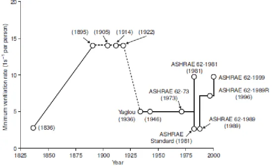
During the last 160 years, in the USA, there has been a constant review of the recommended ventilation flow rates for an occupied building. Figure 3 shows these reviews which reflect the lack of knowledge of the optimum flow rates necessary to keep a building with good health and comfort criteria. The constant adjustment of policies can also have origin in constant changes in the building design, lifestyle, technological development or due to the change in the relative cost of energy (Awbi 2003).

(21)

Figure 3 Changes in the minimum ventilation rates in the USA (Awbi 2003).

Nowadays there are recommendations and standards that should be followed during the design of ventilation systems. ASHRAE Standard 62-1999 (1999) gives air flow rate as function of the number of occupants for different type of building uses (Table 1). For different building uses, different occupation criterion exists in the regulations. As example, in The Netherlands the minimum area per person for an office building is 7 m2 (NEN 1824:2010 2010).

(22)

2.5. Age of air and air exchange efficiency

To characterize the ventilation effectiveness of fresh air distribution, the local mean age of air (τ) can be used. This is a statistical measure of the time it takes for a parcel of air to reach an arbitrary point after it has entered an enclosure (Sandberg 1981).

Another air quality indicator used in this field is the air exchange efficiency which is defined as the efficiency of airflow flushing a volume with external air (Hang et al. 2009). It represents the ratio between the minimum time for replacing the air in the room (τn) and the average time for air

exchange (τexe). The minimum time for replacing the air in the room is the time needed to replace

the whole volume using a certain ventilation flow rate and the average time for air exchange is the actual time the air is in the enclosed space. It is known that τexe is twice the local mean age of air

(τ) (Etheridge & Sandberg 1996). It can be represented by Equation (1):

The air exchange efficiency is related to the flow type as Table 2 shows. In an ideal piston flow, the air enters a space at one end, moves through it with the same velocity on parallel paths and the air exchange efficiency is 100%. In a perfect mixed system, where the conditions are uniform throughout the enclosure at a given moment, the air exchange efficiency is 50%. In a short-circuiting situation, where the major part of the flow flushes quickly through a small portion of the volume and only a small part flushes through the entire enclosure, the air exchange efficiency is less than 50% (Hang et al. 2009; Hang and Li 2011).

Table 2 Air exchange efficiency for characteristic room ventilation flow types (Novoselac & Srebric 2003).

2.6. Carbon dioxide (CO

2

) concentration

There are many types of contaminants and for each one, there exists a different exposure limit depending on the duration a person is exposed to the pollutant (Awbi 2003). When designing a ventilation system, it is necessary to identify the contaminants, the sources and the acceptable concentrations in indoor air, so the proper flow rate can be specified to dilute or extract these contaminants.

One of these contaminants is carbon dioxide (CO2) and in a building it is mainly produced by

human respiration. CO2 is a way to measure the staleness of indoor air due to the fact that it

𝜀_𝑎 = 𝜏𝑛 𝜏_𝑒𝑥𝑒=

𝜏_𝑛

(23)

cannot be filtered, adsorbed or absorbed, contrasting with other contaminants. According to Fanger et al. (1988), CO2 is not a good predictor of air quality perceived by people entering a

space, and for this reason special attention should be given to the proper design of the ventilation systems.

CO2 is present in the outdoor air in a volume average of 0.04% and the expired air contains 4.4%

by volume of CO2. According to Awbi (2003), the rate of production of CO2 by respiration is related

to the metabolic rate of a person (Equation (2)), where G is the CO2 production in l h-1, M the

metabolic rate (W m-2) and A is the body surface area (m2). As an example, an average sedentary adult (M = 70 W m-2 and A = 1.8 m2) produces 18 l h-1 of CO2.

The maximum recommended concentration of CO2, for 8h occupation is 0.5%. Although it is known

that concentrations over 0.1% can cause discomfort and headache (Sundell 1982).

After analysing these numbers it is possible to understand that the CO2 concentration has an

impact in the air quality of a room. For this reason it is important to take into account the population density, the outdoor flow rate and the efficiency of the ventilation system during the design phase. In Table 3, it is possible to observe the outdoor flow rates necessary to maintain 0.5% and 0.25% CO2 concentration for different metabolic rates, assuming a perfect mixing of the

CO2 with the room air. When this perfect mixing does not occur, higher values of ventilation rate

should be used.

Table 3 Outdoor air requirements for respiration (BS 5925 1991).

𝐺 =4 × 10

−5_𝑀𝐴

(24)

(25)

3. Methods for predicting ventilation performance for buildings

The ventilation performance usually can be predicted or evaluated by analytical and empirical solutions, experimental measurements (small and full scale) and computer simulations (multizone models, zonal models and computational fluid dynamics).

Analytical models are the oldest method to predict ventilation performance. In the present days, the contributions for research literature are minimal due to the fact that it has been developed for decades. Although, it is still very useful nowadays due to its simplicity, rich in physical meaning and little computer requirements. Analytical models are derived from fundamental equations of fluid dynamics, heat transfer and chemical-species conservation equations, and use simplifications in the geometry and thermo-fluid boundary conditions to calculate the solutions. Empirical models, as the analytical models, are derived from conservation equations. Often, these models were developed using data from experimental measurements or advanced computer simulations to obtain coefficients that make empirical models successfully work. Empirical models are effective, cost-cutting tools to predict ventilation performance. As the analytical models, empirical models are very case dependent and their contribution to the research literature in the last few years has been scarce after a few decades of development. However, these methods are less suitable for practical applications in specific environments (van Hooff et al. 2011) and its capabilities to determine the room airflow in different types of openings, in complex geometries or with different heat sources are doubtful (van Hooff 2012).

Small-scale experimental models use measuring techniques to predict or evaluate ventilation performance of a reduced-scale building or room. These models are effective and economical to use when comparing to the full-scale experimental models. Nevertheless, attention has to be given to guarantee that important dimensionless flow parameters are equal to the ones existing in the real buildings or rooms. It can also be challenging to scale down complex flow geometry. According to Chen (2009), these models were mainly used to validate analytical, empirical or numerical models, which were then scaled up to real buildings to study the ventilation performance. The full-scale experimental models, as the small-scale ones, are usually used to validate numerical models (mainly CFD models) and then to predict ventilation performance or design ventilation systems. The full-scale experimental models can be divided in laboratory experiment or in-situ measurements. These models give the most realistic prediction of ventilation performance for buildings (Chen 2009). On the other hand, these experiments are very expensive, time consuming and are not free from errors.

The multizone network models are mostly used to predict air exchange rates and airflow distributions between zones of a building and between the building and the outdoors, with or without mechanical ventilation systems. These models assume that the momentum effect can be neglected. Uniform air temperature and uniform chemical-species concentration in a zone are also assumed. The multizone models seem to be the only tool to obtain meaningful results for predicting ventilation performance in an entire building (Chen 2009). Zonal models divide a room into a limited number of cells to calculate the temperature in each cell, in opposite to the well-mixing assumption of the multizone network models. Also, these models predict temperatures in

(26)

large indoor spaces or in rooms with stratified ventilation system. These models do not solve the momentum equation therefore they are mainly used for flows with weak momentum forces in the room air.

3.1. Computational Fluid Dynamics (CFD)

Computational Fluid Dynamics (CFD) refers to solving and analyzing fluid flow problems numerically. CFD solves a set of partial differential equations for the conservation of mass (continuity equation), momentum (Navier-Stokes equations), energy, chemical-species concentrations and turbulence quantities. CFD models have become increasingly used in predicting ventilation performance despite of still having some uncertainties in the models. It requires appropriate knowledge on fluid mechanics and demands high computer resources because of i) the awareness of the power of these models is increasing; ii) the increase in the computational resources and; iii) the increasing availability of user-friendly software interfaces. The importance of CFD in all domains of engineering has been increasing and its use for studying the indoor air quality or thermal comfort are examples of its significance. The study of indoor air quality with CFD models is generally divided in three categories (Chen 2009):

 indoor air quality studies in spaces with non-uniform distributions of contaminant concentrations;

 natural ventilation designs;

 investigations on stratified indoor environments.

The use of CFD models in ventilation performance of indoor environments have been largely studied due to difficulty in predicting it with other models (Chen 2009). Example of this is the design of natural ventilation which is very challenging because of the constant change of wind speed and direction resulting from the impact of adjacent buildings (Chen 2009). Additionally there are difficulties in modeling the interaction at the openings of an enclosure; between the outdoor wind flow around the building and the indoor airflow inside the building (Ramponi & Blocken 2012b).

As stated before, CFD is a powerful tool but only if used correctly. Otherwise it can be a dangerous tool giving incorrect results and for this reason many professionals mistrust CFD results. It is necessary to always question the accuracy and reliability of the CFD results because CFD results are wrong until proven otherwise (Blocken 2014).

3.1.1. Fundamental equations

There is a set of fundamental equations that are the basis of CFD: the continuity equation (Equation (3)) and the momentum equations known as the Navier-Stokes equations (in modern CFD literature, the Navier-Stokes equations may refer to the entire system of equations for the solution of the viscous flow: continuity, momentum and energy). The Navier-Stokes equations are three coupled, non-linear second order partial differential equations describing the fluid flow. For

(27)

an incompressible, viscous, isothermal flow of a Newtonian fluid, the equations are given by Equation (4)-(6). z: ∂w_∂t + {u∂w_∂x + v∂w_∂y + w∂w_∂z} = −1_ρ∂p_∂x+ 𝑣 {∂ 2_w ∂x2 + ∂2_w ∂y2 + ∂2_w ∂z2} + g (6) x, y, z: Cartesian co-ordinates

u, v, w: velocities along the Cartesian axes x, y, z [m s-1]

p: pressure [Pa]

v: kinematic molecular viscosity [m2 s-1] ρ: density [kg m-3

]

g: gravitational acceleration [m s-2]

There are three main methods to predict the turbulent flow: Direct Numerical Simulation (DNS), Large Eddy Simulation (LES) and Reynolds-Averaged Navier-Stokes equations (RANS). In the first method - DNS - the Navier-Stokes equations are solved for all the motions in the turbulent flow. This method is only used with low Reynolds numbers and simple geometries, due to its high demand of computer resources. In LES, the Navier-Stokes equations are filtered, separating the large-eddies from the small turbulent eddies, removing these ones. The largest scale motions of the flow are solved and the small-scale motions are modeled by a subgrid-scale model. This method is less accurate than DNS but more accurate than the RANS. In RANS method, the equations are derived by averaging the Navier-Stokes equations. In this method, only the mean flow is solved while all scales of turbulence have to be modeled using the so-called turbulence models. The RANS method has been the most widely used in the field of numerical computation of air flow inside buildings.

3.1.2. Reynolds-Averaged Navier-Stokes equations – turbulence models

As aforementioned, the RANS methods require the modeling of all scales of turbulence. As a consequence of the averaging process, Reynolds stresses are created and the RANS equations do

∂ρ ∂t+ ∂ ∂x(ρu) + ∂ ∂y(ρv) + ∂ ∂z(ρw) = 0 (3)

x: ∂u_∂t+ {u∂u_∂x+ v∂u_∂y+ w∂u_∂z} = −1_ρ∂p_∂x+ 𝑣 {∂ 2_u ∂x2+ ∂2_u ∂y2+ ∂2_u ∂z2} (4) y: ∂v ∂t+ {u ∂v ∂x+ v ∂v ∂y+ w ∂v ∂z} = − 1 ρ ∂p ∂x+ 𝑣 { ∂2_v ∂x2+ ∂2_v ∂y2+ ∂2_v ∂z2} (5)

(28)

not form a closet set. Hence, approximations have to be made using turbulence models. A given turbulence model is unable to fully represent all turbulent flows therefore different turbulent models have been developed and they should be carefully chosen for each different case. There are two main eddy-viscosity turbulence models: the k-ε model and the k-ω model and each one has different revised versions (i.e. RNG k-ε or SST k-ω).

In the k-ε models (in the standard and in the revised ones) there are two transport equations to represent the turbulent properties of the flow. In these equations there are two transported variables: the turbulent kinetic energy, k, and the turbulent dissipation rate, ε. In general, the revised models of the standard k-ε model are more reliable and accurate for a wider range of flows than the standard k-ε model. For example, the renormalization group (RNG) k-ε model includes additional terms and functions in the transport equations of k and ε, and it was developed to account for the effect of smaller scales of motion. This model has a good performance in indoor air simulations (Ramponi & Blocken 2012b).

In the k-ω models (standard and in the revised ones) there are two transport equations to represent the turbulent properties of the flow. In these equations there are two transported variables: the turbulent kinetic energy, k, and the specific dissipation rate, ω. The k-ω model is well suited for simulating flow in the viscous sub-layer. The shear stress transport (SST) k-ω model is an example of a revised version of the standard k-ω model. The SST k-ω model is a combination of the k-ω and the k-ε model, with the first one modeling flows near the walls and the second one in the free steam.

In indoor air flow modeling, the RNG k-ε model has a better performance than the standard k-ε model (Ramponi & Blocken 2012b; Evola & Popov 2006; Mistriotis et al. 1997; Bartzanas et al. 2007; Kobayashi, T. et al. 2009) and the SST k-ω model has been found to perform even better than the RNG k-ε (Ramponi & Blocken 2012b).

3.1.3. Computational domain and grid

In the preprocessing of a CFD study a geometrical model of the building is made and it is placed in a computational domain, which is then meshed and on which boundary conditions are applied. The computational domain in the CFD simulation for building engineering represents the built area that is investigated. Meshing the computational domain consists on the division of the domain in a large number of control volumes or cells. There are two main types of mesh structures: structured meshes and unstructured meshes (Figure 4). The first ones are quadrilateral cells in 2D and hexahedral cells in 3D (the domain is divided in rectangular areas) and are usually used for simple geometries. The unstructured meshes are composed by triangular and/or hexahedral cells in 2D and tetrahedral, prism, pyramid and/or hexahedral cells in 3D and, in general are used in complex geometries. They can be automatically generated with grid generation software but this often provides poor grid quality. When meshing a domain it is recommended that a maximum expansion rate of 1.2-1.3 is used between cells.

(29)

Figure 4 Different types of control volumes or cells (Ansys 2009).

The computational domain in the CFD simulation for building engineering represents the built area under investigation. The most used discretization technique, due to its versatility, is the control volume method. In this method, each cell of the computational domain is a finite volume, and in its centers the governing equations and the equations of the turbulence model are solved. It is necessary to accurately model the areas where the flow has a bigger impact and in the areas of interest, on which the higher level of detail (higher number of cells) should be present. In buildings, where the areas of interest are usually situated, at least 10 cells should be used per building side, as a starting grid resolution (Franke et al. 2007). Therefore, it is important to perform a grid-sensitivity analysis to understand the impact of the mesh resolution on the results (Franke et al. 2007).

It is necessary to guarantee that the computational domain is large enough to avoid the influence of the boundaries (inlet, outlet, bottom, top and sides of the domain) on the flow around the buildings. According to the best practice guidelines (Franke et al. 2007; Tominaga et al. 2008), the size of the computational domain should be 5 times the building height (5H) or more away from the building to the sides and to the top of the building. The outflow boundary condition should be set at least 15H behind the building to allow the flow re-development. The distance between the inlet boundary and the building should be 5H (Franke et al. 2007; Tominaga et al. 2008). Blocken et al. (2007a,b) recommended a reduction of this inlet distance from 5H to 3H of the building height to limit the development of unintended streamwise gradients.

(30)

3.1.4. Boundary conditions

In simulating of the lower parts of the atmospheric boundary layer (ABL) (0-200m) an accurate description of the flow near the ground surface is required. To describe this flow it is required to have the inlet profiles of the mean wind velocity, turbulent kinetic energy, turbulence dissipation rate (k-ε models) and specific dissipation rate (k-ω models), which are generally fully developed, neutrally stratified and should represent the roughness characteristics of the terrain upstream of the inlet plane. To define these profiles it is necessary to have the vertical profiles of mean wind speed (U) and streamwise turbulence intensity (Iu), which can be obtained from the measured

data when available.

The inlet profile of the mean wind velocity (U) is described by the logarithmic law (Equation (7)), where u* is the friction velocity (represents the magnitude of de fluctuations in the velocity, in the turbulent boundary layer), k is the von Karman constant (0.42), z the height coordinate and z0 is

the aerodynamic roughness length.

The vertical distribution of the turbulent kinetic energy (k), measure of the energy associated with the turbulent fluctuations in the flow, can be calculated using Equation (8), where the standard deviations of the turbulent fluctuations (σ) in the three directions are needed (u, v, w).

The standard deviations of the turbulent fluctuations are related to the turbulence intensity: 𝐼 = 𝜎

𝑈. However, only the streamwise turbulence intensity component (Iu) is usually measured and

assumptions for the other two components have to be made:

 Assumption 1. 𝜎𝑢2≫ 𝜎𝑣2≈ 𝜎𝑤2, which results in:

 Assumption 2. 𝜎𝑢2≈ 𝜎𝑣2+ 𝜎𝑤2, which results in:

 Assumption 3. 𝜎𝑢2≈ 𝜎𝑣2≈ 𝜎𝑤2, which results in:

In conclusion, the relationship between the turbulent kinetic energy (k), the streamwise intensity component (Iu) and the wind speed (U) is given by Equation (12), where a is equal to 0.5, 1 or 1.5.

The best practice guidelines by Tominaga et al. (2008) recommend the use of a = 1. 𝑈(𝑧) = 𝑢∗ 𝑘 ln ( 𝑧 + 𝑧0 𝑧 ) (7) 𝑘(𝑧) =1 2(𝜎𝑢2(𝑧) + 𝜎𝑣2(𝑧) + 𝜎𝑤2(𝑧)) (8) 𝑘(𝑧) =1 2(𝐼𝑢(𝑧) 𝑈(𝑧))2 (9) 𝑘(𝑧) = (𝐼_𝑢(𝑧) 𝑈(𝑧))2 ₍₁₀₎ 𝑘(𝑧) =3 2(𝐼𝑢(𝑧) 𝑈(𝑧))2 (11) 𝑘(𝑧) = 𝑎 (𝐼_𝑢(𝑧) 𝑈(𝑧))2 ₍₁₂₎

(31)

The vertical profile of the turbulence dissipation rate (ε) is defined by Equation (13), where z0 is

the aerodynamic roughness length. The specific dissipation rate (ω), which is derived from the turbulence dissipation rate (ε) and from the turbulent kinetic energy (k), is given by Equation (14), where Cµ is an empirical constant considered equal to 0.09.

It is also necessary to do an accurate description of the flow near the ground surface. Blocken et al. (2007b) described four requirements that should be satisfied, when the wall roughness is expressed by an equivalent sand-grain roughness height (ks):

1. A high mesh resolution should exist in the vertical direction adjacent to the bottom of the computational domain;

2. The ABL flow should be horizontally homogenous on the upstream and downstream regions of the computational domain;

3. The distance from the bottom of the domain to the centre point of the wall adjacent cell (yp) should be larger than the roughness height (ks), yp > ks;

4. The relationship between the sand-grain roughness height (ks) and the corresponding

aerodynamic roughness length (z0) should be known.

Blocken et al. (2007b) derived this relation and for Fluent (a commercial CFD software) is expressed by Equation (15), where Cs is the roughness constant.

The selection of the correct ks and Cs values should be carefully taken into account, because of

their importance to reduce unintended streamwise gradients in the flow profiles in the simulation. 𝜀(𝑧) = (𝑢 ∗₎3 𝑘(𝑧 + 𝑧0) (13) 𝜔(𝑧) = 𝜀(𝑧) 𝐶𝜇𝑘(𝑧) (14) 𝑘_𝑠 = 9.793 𝑧0 𝐶_𝑠 (15)

(32)

(33)

4. Overview of previous studies

4.1. Wind tunnel studies

Wind tunnel studies to examine cross-ventilation flow characteristics in a single-zone building were conducted by Karava (2008) and Karava et al. (2011). The wind tunnel experiments were done with a method based on particle image velocimetry (PIV). This method is based on non-intrusive measurements and it allows to obtain whole field functions unlike other wind tunnel techniques which are limited to single-point intrusive measurements (Karava et al. 2011).

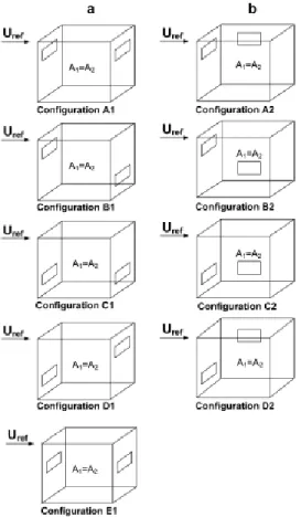
Within this study, the wind tunnel experiments were performed in the Boundary Layer Wind Tunnel of the Building Aerodynamics Lab at Concordia University (Stathopoulos 1984), which dimensions are 12 meter long and a cross section of 1.8 x 1.8 m2. Building models with a scale 1:200 with the dimensions W x D x H = 100 x 100 x 80 mm3 (full scale dimensions of 20 m x 20 m x 16 m) were built with sheets of 2 mm cast transparent polymethylmethacrylate (PMMA). Different configurations were tested, changing the position of the windows (in opposite or adjacent walls and near the bottom, in the middle and near the top of the walls) and different opening areas (wall porosity, w.p. = Aopening/Awall, between 2.5% and 25%). In all these configurations the window

height was fixed (18 mm) changing only the length. The different configurations are shown in Figure 5 and in Table 4.

Figure 5 Opening configurations considered for studying the effect of wall porosity and opening location on ventilation flow rate (Karava et al. 2011).

(34)

Table 4 Study considerations and range of variables (Karava et al. 2011).

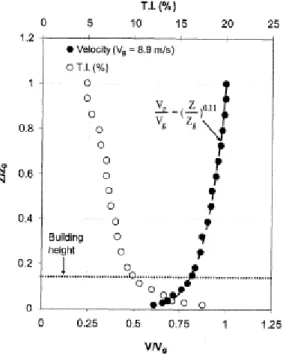
The experiments were performed with a maximum wind-tunnel speed of 8.9 m s-1 and an open terrain was simulated with a roughness length (z0) of 0.005 m. The incident velocity and

turbulence intensity were measured with a hot-film probe at the building position and are shown in Figure 6. At the building height (H = 80 mm) a reference mean wind speed and a streamwise turbulence intensity were measured, being Uref = 6.97 m s-1 and TI = 10%.

(35)

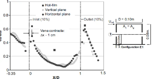
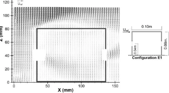
In the referred works, basic airflow features were examined in the building space, which can be helpful in the development of models for natural ventilation analysis and design. Figure 7 shows an example, where the x-component of the velocity (normalized by the velocity at the building height) on the center-line directly between the openings. A comparison between the values of PIV data for measurements in the horizontal and vertical plane and single-point hot-film data is shown and it can be noticed that there is a good agreement between both PIV measurements (horizontal and vertical plane). Instead, the hot-film measurements tend to overestimate the velocity near the inlet opening and in the center of the building, which can be justified by high turbulence intensities (hot-film measurements cannot distinguish between the mean velocity and the fluctuating components of the velocity, which exists in highly turbulent flows) in this flow region (over 30%). Figure 8 shows the cross sectional view of the mean velocity vector field on a vertical mid-plane. It can be seen that the main jet passes through the center of the opening, while there are slower moving zones above and below this flow region. After the inlet region, the main jet is accelerated and has a downwards direction caused by the location of the opening (in the mid-height of the building) and by the existence of an upstream recirculating flow (standing vortex) near the ground outside the building model. There is also a recirculation zone below the inlet jet. In the central region the flow decelerates and it accelerates again at the outlet opening. At this opening, the jet is directed upwards, due to the existence of a recirculation flow in the wake region of the building. Although, not all the jet exits the building. Some of the faster moving flow goes up to the ceiling where it travels in the opposite direction of the flow until it reaches the windward façade, being directly downwards.

Figure 7 Profile of x velocity component on the center-line directly between the inlet and outlet openings (PIV measurements on a horizontal and vertical plane and single-point hot-film data) (Karava et al. 2011).

(36)

Figure 8 Cross-sectional view of mean velocity vector field on a vertical mid-plane with 10% wall porosity (Karava et al. 2011).

The flow was also studied for the other building configurations. Karava (2008) and Karava et al. (2011), when studying the different building configurations, concluded that configurations with higher airflow rates in cross-ventilation are found in cases of:

(i) Symmetric openings.

(ii) Inlets located at the mid-height of the building or above.

(iii) Inlet-to-outlet area ratio lower than one (inlet opening smaller than the outlet opening).

These configurations can be used for space or building fabric cooling. On the other hand, if thermal comfort is the objective of the cross-ventilation, configurations with the inlet opening larger than the outlet opening should be used (Karava et al. 2011). In all the different configurations, two different zones are found: the main jet and the recirculation zone. These two zones are essential when designing systems which take into account the local heat transfer inside the room.

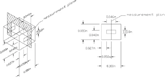
Chu et al. (2010) made an experimental study of wind-driven cross-ventilation in partitioned buildings. This study was conducted in an open-circuit, blowing wind tunnel. It consisted in testing a cubic shape building with square-shaped openings with different diameters, with a partitioned plate on the middle of the room with different opening positions and diameters (Figure 9). In this study, it was found that the inlet velocity increases as the porosity of the internal wall increases. Although when the internal porosity is over 10% the inlet velocity stabilizes at a constant value of

(37)

It was concluded that the maximum ventilation rates were obtained when the inlet and outlet openings had the same size, regardless of the internal partition. It was also concluded that the ventilation rate of the partitioned buildings was always smaller compared to a building without internal partitions, due to the fact that the partitions reduced the pressure difference between the interior and the exterior of the building. This paper concludes, then, that the openings (inlet, outlet and interior) can control the ventilation rate in the building.

Figure 9 Schematic diagram of experimental setup (left). Geometry of internal partition wall (right).

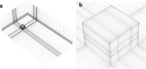
Bangalee et al. (2013) and Chu and Chiang (2013) performed wind tunnel studies to compare with CFD simulations. The first used flow visualization (to observe the three-dimensional and turbulent flow), PIV measurements (to measure the velocity flow fields, similar to the work of Karava (2008) and Karava et al. (2011)). While the second performed a wind tunnel experiment using the flow condition and building dimensions used by Karava (2008) and Karava et al. (2011). Further information on their works can be found in the next section.

4.2. CFD studies

Based on the work by Karava (2008) and Karava et al. (2011) several CFD studies have been performed. Ramponi and Blocken (2012a), studied the impact of different building opening configurations: two different wall porosity ratios (5% and 10%) and different facing opening positions (in the center and near the ground of the building). The results showed the importance of choosing the appropriate grid resolution and the necessity to use at least second-order accurate discretization schemes to reduce the effect of numerical diffusion. The study concluded the importance of choosing the correct amount of physical diffusion due to its impact on the results. Ramponi and Blocken (2012b) performed a set of simulations to analyze and evaluate the impact of different computational parameters on coupled CFD simulations of wind-induced cross-ventilation. In this study the openings (both with 10% wall porosity) were situated on the center of the two opposite walls (Figure 10). The dimensions of the computational domain were based on the best practice guidelines by Franke et al. (2007) and Tominaga et al. (2008) apart from the upstream length that was reduced to 3 times the building height to avoid the development of unintended streamwise gradients (Blocken et al. 2007a,b). Thus the width of the computational domain had a cross section defined as WD = W + 10H and the height defined as HD = H + 5H, where

(38)

W is the width of the building and H the building height. The computational grid was created

based on the surface-grid extrusion technique developed by van Hooff & Blocken (2010), using a maximum stretching ratio of 1.2 controls the cells surrounding the building model. The roughness length was equal to 0.025 mm, the sand-grain roughness height and the roughness constant were calculated using the Equation (15), and were equal to ks = 0.28 mm and Cs = 0.874. The simulations

were performed with Fluent 6.3.26, and the reference case solved the 3D steady RANS equations with the SST k-ω model. In the reference case, a SIMPLE algorithm was used for pressure-velocity coupling, and second order discretization schemes were used. The value of a in the turbulent kinetic energy equation was assumed to be 1, and the simulation was stopped when convergence was reached.

Six parameters were tested in this work by Ramponi and Blocken (2012b), and are resumed in Table 5:

 the size of the computer domain, changing the width (WD = W + 2d, where d is the

distance from the side walls and the roof to the side and top of the computational domain) and the height (HD = H + d) of the computational domain. The best practice

guidelines used in the reference case outperformed the other cases when comparing with the experiments by Karava (2008) and Karava et al. (2011), showing that the results are independent of the cross-sectional dimensions;

 the computational grid resolution analysis showed a good grid convergence between the two higher grid resolutions and also accurate results compared to the experimental ones;

 the inlet turbulent kinetic energy of the atmospheric boundary layer analysis revealed a significant impact of this parameter on the results, being the simulations which used a = 1 that had the best performance, comparing to the results of a = 0.5 (underestimated) and a = 1.5 (overestimated);

 different turbulence model were tested and the SST k-ω model was the one with the best results followed by the RNG k-ε model;

 the importance of using the appropriate discretization scheme (second-order) was proven;

 the convergence criteria analysis showed that a sufficiently stringent convergence criteria should be used (the ones suggested by the CFD codes are often insufficient).

(39)

Figure 10 Building model and measurement plane used for PIV measurements by Karava et al. (2011).

Table 5 Overview of computational parameters for sensitivity analysis with indication of the reference case (Ramponi & Blocken 2012b).

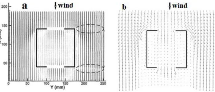
Bangalee et al. (2013) performed a study using flow visualization (to observe the three-dimensional and turbulent flow), PIV measurements (to measure the velocity flow fields, similar to the work of Karava (2008) and Karava et al. (2011)) and CFD techniques (to predict the internal flow patterns and the ventilation flow rates). A good agreement between the different data was achieved. The flow fields of four different building configurations (Figure 11) were also compared. The numerical simulations were performed assuming that the system is steady, incompressible, viscous, turbulent, non-buoyant and three dimensional. Water was considered as the working fluid (25ºC and 1 atm), using the RNG k-ε turbulence model with a fully structured grid. This study concluded that using multiple openings on both sides of the room increases the ventilation flow rate and ensures a better interior air replacement. Moreover, for fixed wall porosities higher flow rates are obtained when the openings are located in the middle of the walls (the ventilation rate for Case 2 is 34% smaller than for Case 1). Although it is important to notice that the interior air replacement is higher for Case 2 (with oblique opening positions) comparing to Case 1 (facing opening positions) due to the higher interaction of the entering flow and the interior air.