Residence Time Distribution Studies in Continuous Thermal
Processing of Liquid Foods: a Review
A. Pinheiro Torres” & F. A. R. Oliveirah*
“Escola Superior de Biotecnologia. R. Dr Ant6nio Bernardino de Almeida, P-3200 Porte.
Portugal
“lnstituto Inter-Universitkio de Macau, Pakkio da Penha, Macau
(Received 15 January 1997; accepted 17 February 199X)
ABSTRACT
This paper presents a review on residence time distribution (RTD) studies in continuous thermal processing of liquid foods. The theoretical basis of the Danckwerts analysis is summarized, as well as the most important flow models,
with special emphasis on tubular systems. Methods for experimental determination, modelling and estimation of RTD are critically described. While main design objectives in continuous thermal processes may be guaranteed by a proper minimum residence or holding time, process optimization requires the knowledge of the residence time distribution. Both concepts are reviewed and discussed. A significant scatter was noticed among published results and the need ,for a systematic work is clear It was concluded that future research should focus on studies at pasteurizationlsterilization temperatures, as well as on studies conducted with real food products or model food systems with FIO~I-
Newtoniun flow bchaviour: Furthermore. information relating RTD to processing conditions would be a useful tool for process optimization. 0 1998 Elsevier Science Limited. All rights reserved.
NOMENCLATURE c Concentration, in the time domain (g I ‘) c Concentration, in the Laplace domain (g s- ‘)
n Tube diameter (mm or m)
D Axial dispersion coefficient (m’ s ~~ ’ )
*To whom correspondcncc should be addressed. Fax: +X53-725 5 17; e-mail: fernanda@
2 A. Pinheiro Ton-es, E A. R. Oliveira Da
E(O)
E(t)
fF
G k L & m t?Z’; c Pe Pe,Q
Re s SC t T V V fDamkohler number (dimensionless)
Residence time distribution function (dimensionless) Residence time distribution function (s ~ ‘)
Friction factor (dimensionless)
Cumulative residence time distribution function (dimensionless) System transfer function (dimensionless)
Reaction rate constant (s-l, min-‘) Tube length (m)
Laplace transform
Exponent for the velocity distribution (dimensionless) ith order ordinary moment (s’)
Flow behaviour index (dimensionless) Natural number
Peclet Number Pe = vL/D (dimensionless) Axial Peclet number Pe, = vd/D (dimensionless) Flow rate (m” s-‘, 1 hh’)
Reynolds number Re = pvd/,u (dimensionless) Independent variable in the Laplace domain (s-l) Schmidt number SC = ,u/pD (dimensionless) Time (s, min)
Temperature (“C, K) Velocity (m s- ‘) Volume (1, m”)
Mean residence time (s, min)
Greek symbols
cs2
Subscripts
Parameters
Relative measure of skewness Relative measure of kurtosis Dirac function Efficiency Variance (s2$ Skewness (s- ) Kurtosis (s4) Dimensionless time
Dimensionless mean residence time Mean holding time (s)
amb ave e i min pred Ambient Average Output, exit Input, initial Minimum Predicted
Residence time distrihutiorz studies 3 INTRODUCTION
Fluid flow can be described by two different approaches: fluid mechanics theory (Taylor, 1954; Brodkey, 1967) or residence time distribution (RTD) theory (Danck- werts, 1953; Zwietering, 1959). Books and chapters have been written on residence time distribution (Levenspiel, 1972; Wen & Fan, 1975; Hill, 1977; Fromment & Bischoff, 1979; Fogler, 1986). This concept has been widely applied to chemical processes and more recently has gained a significant interest in the pollution and environmental field, as well as in several biotechnology applications. In general, one can say that RTD analysis is an empirical yet simple approach to describe any process that involves fluid/particulate fluid flow. In the food field, RTD analysis has been applied for assessing the effects of processing parameters on the flow charac- teristics in different processes, such as extrusion cooking (Yeh et al., 1992; Zulichem ef al., 1973) or fermentation processes (Hubbard & Williams, 1977; Kulozik et al.,
1992). In food engineering however, RTD has its widest application in aseptic processing (Bailey & Ollis, 1986; Burton, 195Sa; Rao & Loncin, 1974a, 1974b; Lin,
1979). Between 1969 and 1994, 165 references were found in the Food Science and Technology Abstracts (FSTA), corresponding to an average of five papers per year. a relatively low number if one considers the impact these studies may have on process assessment and optimization and on diagnosing malfunctions when operat- ing processing equipment (Levenspiel, 1972).
Aseptic processing is commonly applied to a wide range of liquid foods (milk, fruit juices and concentrates, cream, yoghurt, wine, salad dressing, egg and ice cream), foods containing small particles (cottage cheese, baby foods, tomato products, soups and rice desserts) and its application to large particulate foods is currently a major topic of research (Lee et ul., 1995; Singh & Lee, 1992). Systems for the aseptic processing and packaging of fluid foods have been extensively reviewed by Hersom (1985). Continuous aseptic processing involves three major steps: heating, holding and cooling. The food is aseptically processed and then also aseptically packed. Holding temperatures may vary from 65 to 150°C. Holding times may vary from a few seconds to several minutes and may be attained by choosing an appropriate holding tube length, that is dependent on flow rate.
RTD studies in aseptic processing of foods were first applied to estimate the level of microbial contamination after processing (Bateson, 1971; Burton, 1958b; Burton
et al., 1958; Milton & Zahradnik, 1973; Veerkamp et al.. 1974; Wennerberg, 1986).
RTD can also be applied to assess mixing between two miscible liquids pumped in succession through a pipe (Sjenitzer, 1958), which is a common procedure in the start-up of aseptic processing units. However, the full potential of RTD studies relies on its applicability to optimization studies. The main advantage of continuous thermal processes when compared to in-container pasteurization or sterilization arises from the quality improvement of the product due to shorter heating and cooling rates (Hersom, 1985). Full potential of continuous thermal processes is yet to be attained and depends on the ability of controlling flow characteristics in processing equipment (Lin, 1979). In continuous thermal processing, time/tempera- ture conditions are constrained by product safety requirements (microorganism or enzymes which may cause degradation or health hazards to be reduced to a target level), while product quality (e.g. texture, colour) should be kept as high as possible. Product safety is related to the minimum residence time (mRT), while product quality relates to the RTD of the product in the system. Optimization of aseptic
4 A. Pinheiro Torres, E A. R. Oliveira
processes may therefore be achieved not only by choosing adequate time/tempera- ture conditions, but also by controlling flow characteristics. RTD theory may also be applied for process optimization in terms of capital and operation costs (Malcata, 1991), though process optimization in terms of product quality is much more important when dealing with food products (Burton, 1958b; Holdsworth & Richard- son, 1986; Kessler, 1989; Lund, 1977; Maesmans et al., 1992; Rao & Loncin, 1974b). This paper reviews RTD in continuous thermal processing of liquid foods focus- ing particularly on the following topics: (i) methods used for experimental measurement of RTD; (ii) methods available for data treatment and analysis; (iii) RTD modelling. One of the most important parameters of RTD in continuous thermal processing is the minimal residence time of the fluid (mRT), as it is directly linked to product safety. Therefore, on this paper mRT and RTD studies will be considered separately, depending whether only mRT or the whole distribution is considered.
RTD BASIC CONCEPTS
Flow patterns in continuous systems are usually too complex to be experimentally measured or theoretically predicted from solutions of the Navier-Stokes equation or statistical mechanical considerations (Wen & Fan, 1975). Real flow systems often deviate from the ideal flow patterns of plug flow (PF), continuous stirred tank (CST) or flow patterns predicted from mechanistic models (Bosworth, 1948, 1949). Real flow systems were first approached by Danckwerts (1953) on the basis of RTD analysis.
The residence time of an element of fluid is defined as the time elapsed from its entry into the system until it reaches the exit. The distribution of these times is called the RTD function of the fluid E, or E-curve, and represents the fraction of fluid leaving the system at each time, having units of time-‘:’
E(t) = c,(t) s
m c,(t) dt 0
c,(t) being the exit concentration (e.g. of a tracer) at a certain time t. The mean residence time f is the first moment of the distribution:
‘i= X s
t x E(t) dt
0
and is equal to the mean holding time z for vessels with ideal flow: V z= - e
(1)
(2)
(3) with Q standing for product flow rate and V for the system (e.g. the holding tube) volume.In general, to completely characterize an arbitrary distribution function, all moments are required, but most commonly only moments about the mean up to the fourth level are considered relevant. The second centred moment, variance (a’), is an indicator of the spread of the distribution, the third centred moment, called skewness (y”), is an indicator of the asymmetry of the distribution, and finally, the
Residence time distribution studies 5
TABLE 1
Centred Moments About the Mean of the RTD Function*
Moment Definition Formula Relative measure
Variance (t-r)2 x E(r) dr
Skewness I = ?- [ ’ (t--TJ3 xE(t) dt ., 0
;s3 = ‘3 -- 3f,7?‘1+2f7 p, =(;‘i)1/(rT2)t
Kurtosis
*Collected from Hahn and Shapiro (1967).
fourth centred moment, kurtosis (ti4), is an indicator of how heavy-tailed the distri- bution is (Hahn & Shapiro, 1967). These centred moments about the mean are defined in Table 1, and can be easily calculated by using ith order ordinary moments, which are defined as:
s I
in’, = t’ x E(t) dt (4)
0
The first ordinary moment of the RTD corresponds to the mean residence time defined in eqn (2).
The F-curve is a cumulative curve which may also be used to characterize the RTD, and corresponds to the fraction of fluid that has spent less than a time t in the system, being therefore defined as:
i f
F(t) = E(t) dt (5)
0
It is often convenient to use a dimensionless time 0 and the corresponding residence time distribution E(t)) (Levenspiel, 1972):
(I= _f_ and E(O)=s x E(t)
T (6)
The moments of the RTD curve may also be normalized in the same way (Wen & Fan, 1975), though the relative measures of the centred moments in Table 1 are more meaningful and are therefore preferred. The centred moments, as well as the F-curve, are independent of the time units.
For first order reactions under isothermal conditions, RTD information is suffi- cient to predict conversion in the system. In this case, the final average concentration, c,,;,,,, in the exit stream of the system is (Levenspiel & Bischoff,
1963): (‘e.>,\,c = 1 I c,(t) x E(t) dt 0
where c,(t) is the exit concentration at a certain time t.
6 A. Pinheiro Torres, I;: A. R. Oliveira
For other type of kinetics, the system performance cannot be predicted from RTD and kinetic rate information alone, and the degree of mixing in the system has to be taken into consideration (Zwietering, 1959; Rao & Loncin, 1974a).
Another concept that can be useful in RTD modelling and data fitting to experi- mental RTD curves is the transformation of RTD into the Laplace domain. The Laplace transform of a RTD or concentration curve is defined as (Hopkins et al., 1969): 2 C(s)-&(c(t)] - s e-“‘c(t) dt (8) 0
The system response in the Laplace domain, more commonly called the system transfer function G(s), is for any input function defined as:
c_(s)
G(s)- -
Ci(S)
The transfer function for several flow models can be analytically derived from this equation (Hopkins et al., 1969; Wen & Fan, 1975). Also, the ordinary moments in eqn (4) can be directly obtained for any transfer function of a reactor flow model from the following equation (Wen & Fan, 1975):
d”‘G
m’i=(-l)’ lim -
.s+o ds”’
(10)
this being often a more practical procedure to calculate the centred moments, using the formulae shown in Table 1. It can also be shown that the transfer function G(s = k), for a first order reaction with rate constant k, corresponds to the remain- ing fraction of reactant in the exit stream.
METHODS FOR EXPERIMENTAL DETERMINATION OF RTD CURVES
Real foods and model fluids
Model food systems rather than real foods are often used for research purposes, so that problems related to product availability and variability may be overcome. In RTD studies in aseptic processing, model foods should be chosen so that they have rheological and thermal properties similar to those of the food system.
The first mRT experiments on food processes were performed using water as model food (Jordan et al., 1949). Many other authors followed the same approach, although the use of water greatly limits the applicability of the results to a small number of food products and processing conditions (Watson et al., 1960) namely milk, wine and some fruit juices. Only Sancho and Rao (1992) tested other model fluids, such as sucrose and guar gum solutions. In terms of real foods, studies on mRT were reported for milk (Dickerson et al., 1968, 1974; Heppell, 1985; Aoust et al., 1987) milk products (Dickerson et al.), egg products (Kaufman et al., 1968b; Scalzo et al., 1969) and crushed tomato (Rodrigo et al., 1990). Model fluids had a much wider application in RTD determinations; besides water, model fluids tested were: starch solutions (Bateson, 1971) sucrose solutions (Sancho and Rao, 1992) polyethylene glycol (Milton & Zahradnik, 1973), diethylene glycol (Pudgiono et al.,
Residence time distribution studies 7 1992), glycerol/water mixtures (Trommelen & Beek, 1971) and guar gum solutions (Sancho & Rao, 1992). These model fluids cover most rheological behaviour of fluid foods, except for that showing yield stress or very high viscosity. RTD determina- tions on real products were only reported for milk (Cerf & Hermier, 1973; Nassauer & Kessler, 1979; Heppell, 198.5; Janssen, 1994) and coffee cream (Kiesner & Reuter, 1988).
Proposed tracers
Wen and Fan (1975) summarized the basic requirements for selecting a tracer for RTD experiments: (i) it should be miscible and have physical properties similar to those of the fluid under investigation, (ii) it should be accurately detectable in small amounts, so that its introduction does not affect the flow pattern of the main fluid stream, (iii) its concentration should be easily monitored and the recorded signal should be proportional to tracer concentration, and (iv) sorption of tracer by the vessel walls should not occur.
In mRT determinations, a very low limit of detection is required, because only the first response signal is determinant, as stressed by Jordan et al. (1949) that showed that response accuracy was highly dependent on tracer type and concentration. On the other hand for RTD determinations, accurate detection methods are important, and the response should be preferably proportional to the tracer concentration, so that the analysis can be made directly on the response signal (Wen & Fan, 1975).
The various tracers proposed for mRT and RTD experiments in food aseptic processing plants are summarized in Table 2. It is interesting to note that most tracers proposed for real foods, such as for milk products (Dickerson et al., 1968, 1974; Heppell, 1985; Pate1 & Wilbey, 1990) egg products (Scalzo et al., 1969; Kaufman et al., 1968b) and ice cream mix (Thiel & Burton, 1952; Botham, 1952), are only suitable for mRT determinations, because of difficulties in tracer detection using real food systems. For the same reason, tracers proposed for whole RTD experiments (soluble dyes, salt, sodium nitrite, labelled microbials and sucrose) were mostly applied to water and model food products, while for real food products only salt was used as tracer in milk (Nassauer & Kessler, 1979; Heppell, 1985; Janssen, 1994) and coffee cream (Kiesner & Reuter, 1988). It is however interesting to note that in fields other than aseptic processing, tracers have been applied for RTD measurements in real food systems (e.g. radioactive isotopes in extrusion (Zulichem et al., 1973)).
Tracer injection and detection
Perfect injections of tracer have the advantage of producing RTD curves that are easy to analyse statistically and mathematically. Common input functions are perfect impulse, step, purge or pulse. Table 3 summarizes these functions in both time and Laplace domain, as well as the corresponding output functions, which are directly related to the E- or F-curves.
A perfect impulse of tracer is an ideal concept. Minimal deviations from ideality may be in practice obtained by making the time of injection as short as possible (Aris, 1959). A perfect step is easier to perform than a perfect pulse, but the second method is preferred for commercial testing since the processing system is disturbed
8 A. Pinheiro Torres, l? A. R. Oliveira TABLE 2
Tracers Proposed for Residence Time Experiments in Food Aseptic Processing Plants
Tracer type Detection method Experiment Application Reference Soluble dye Salt Sodium nitrite Radioactively labeled microbials Radioisotopes (soluble, suspended or entrapped) Thermal (cold shot) Fluorocarbon 12 (CCl,F,) Sucrose Colorimetry and photometry mRT Photography Electrical conductivity RTD mRT RTD Gries-Ilosvay reagent mRT Gamma radiation RTD Gamma radiation mRT Temperature changes mRT ‘Fluor leak detector’ Polarimetry mRT RTD Water Model food Milk products Milk products Milk Water Water Water Model foods Milk Coffee cream Crushed tomato
Ice cream mix
Water Milk products Egg products Water Egg products Egg products Model foods Jordan et al. (1949) Pudgiono et al. (1992) Heppell(1985) Pate1 and Wilbey
(1990) Dickerson et al. (1974) Roig et al. (1976) Jordan et al. (1949); Anonymous (1950)
Jordan and March (1953)
Sancho and Rao (1992) Nassauer and
Kessler (1979) Kiesner and Reuter
(1988)
Rodrigo et al.
(1990) Botham (1952)
Burton et al. (1958)
Aiba and Sonoyama (1965)
Dickerson et al.
(1968)
Scalzo et al. (1969)
Jordan and Holland (1953) Kaufman et al. Kz%~~!‘et al (1968b) ’ Kaufman et al. (1968b) Chen and Zahradnik (1967)
Residence time distribution studies 0 TABLE 3
Ideal Forms of Tracer Injection (represented in Time and Laplace Domain), and Corresponding Output Functions
_ Input function c,(t) C,(s) c,,(t) lmpulsc Step Purge Pulse Ci h(t) ci (‘, E(t) ci u(t) (‘ ilS (‘1 F(t) c, 11
-WI
ci
(1 - l/s) (‘1 [ 1 -F(t)]Ci [I - u(t -U)] c, {(l--c “‘)/.s} c, [F(t) -F(t -u)]
for shorter times (Levenspiel & Bischoff, 1963). Finally, with respect to the response signal, the step produces an integrated curve which has to be derived to obtain the E-curve for data analysis, thus introducing more computational errors or eventually masking some effects, such as tailing. Therefore, the use of step or purge input functions is not as desirable as impulse inputs.
Pulse or step injection of tracer should always be tested to be sufficiently ideal, but this fact is often overlooked in reported works. If the tracer injection is not ideal, special techniques are required for tracer response analysis, and therefore measurement of the injection response is required for performing a non-ideal injec- tion analysis (Aris, 1959).
Various experimental methods for tracer injection and detection have been developed and optimized and are well described in literature (Anonymous, 1950; Burton, 1958a; Edgerton & Jones, 1970; Jordan & Holland, 1953; Jordan et al., 1949; O’Callaghan & McKenna, 1974). Some studies were made specifically on tracers for real foods, as can be seen in Table 2. Except for Burton (1958a, 1958b) and Burton et al. (1977) who analysed respectively the importance of satisfactory injection and detection conditions on the RTD response, all tracer injection methods were developed for mRT determinations.
Both Aiba and Sonoyama (1965) and Roig et al. (1976) used step injections and obtained RTD curves corresponding to the F-curve. Other researchers used impulse injections, but none reported having checked the ideality of injection, except for Sancho and Rao (1992). Only Kiesner and Reuter (1988, 1990) reported non-ideal injections, and analysed their data accordingly.
MODELS FOR FLOW IN TUBULAR SYSTEMS
mRT models
Although some authors advise experimental determination of mRT (Jordan et al., 1949; Anonymous, 1950), others propose conservative models for estimating mRT from mean holding times z (eqn (3)) in holding tubes (Table 4). The efficiency of a hold tube, I:, can be defined by the following equation (Rao & Loncin, 1974a):
mRT mRT
I:(%) = - xlOO%ora=--- (11)
TABLE4 Models Proposed in Literature for Selection of Minimum Holding Times in Calculating Holding Tube Sizes
Product/ rheological behaviour
mRT Restrictions i:( 701 Reference Newtonian, laminar fiow Newtonian, turbulent flow Pseudoplastic, laminar flow Pseudoplastic, turbulent flow 0% None 50 (a) (0.0336 IgRe + 0.662)~ (b) 0.8~ (c) 2m2/(m + 1)(2m + l)r* (d) 2/(1 +m)l(2+m)s* (n + 1)/(3n + l)z** x 2n0 7s/5.657\1~x ’ w2 n’2p4f’pr*‘2Re)+ 1.204+0.501n-0.1n-“‘4’ t Re > 4000 and 1 <d(cm) < 10 None 4000tRe<2 x lo6 2100 <Re < 12000 0.14 > m > 0.02 12000<Re<20000 m = 0.02 1 > n > 0.2 1 <n < 1.6 1 > n > 0.2 78-96 Palmer and l<n<2.0 71-89 Jones (1976) 78-87 80 82-97 97 50-75 45-50 Dickerson et al. (1968); Rao and Loncin (1974a) Edgerton et al. (1970) Rao and Loncin (1974a) Sancho and Rao (1992) Nassauer and Kessler (1979) Rao (1973) *m = exponent for the velocity distribution (Schlichting, 1960). **n = flow behaviour index. tf= friction factor.
Residence time distribution studies II
and is never below 50% for Newtonian fluids in laminar flow (Table 4). Efficiency below 50% can only occur for dilatant fluids (with flow behaviour index n < 1) in laminar flow (Rao, 1973). In turbulent flow, the theoretical efficiency is always above 70% for any model fluid, as shown in Table 4. There is a lack of models for predicting efficiencies in the transition flow regime zone (2100<Re <4000), as can be concluded from the analysis of Table 4.
The prediction of velocity profiles for fluids in turbulent flow is not as straightfor- ward as for laminar flow. For Newtonian fluids, relationships are reliable, but the available equations for power law fluids have not received adequate experimental verification for food materials (Steffe, 1992). Therefore, models proposed for mRT and efficiency calculations for fluids other than Newtonian are less reliable, as they are mostly derived from the above-mentioned relationships. However, these predict- ive models tend to be conservative, as they are mostly based on ideal flow conditions. Non-ideal flow, due mostly to bends in tubes, entrance and end effects which do not allow fully developed flow conditions, leads to more turbulence and an
mRT consequently higher than that expected from theoretical considerations and corresponding tube efficiency.
Influence of boundary conditions on flow modelling
The procedure used in RTD experiments may determine the resultant tracer output curve. Levenspiel and Turner (1970) illustrated experimentally the effect of injection and measurement of tracer on the shape, mean and spread of the resultant tracer curve. Two possible tracer inputs were considered, namely proportional to the velocity of flow (referred as open boundary condition) or evenly across the Aowing stream (referred as closed boundary condition); tracer was measured by either the mixing-cup technique or by a through the wall measurement. Levenspiel et al. (1970) related the tracer curves obtained by these various techniques, for situations where interaction between neighbouring streamlines is negligible. The features of the main boundary conditions are discussed by Wen and Fan (1975).
RTD models commonly applied for tube flow
Theoretical models for fluid flow in tubular systems (as holding tubes) at isothermal conditions are summarized in Table 5. These models were divided in mechanistic (derived from fluid mechanics theory) or stochastic (based on probability theory) models.
Ideal RTD models like the plug flow (PF) and ideal continuous stirred tank (CST) rarely reflect a real situation with enough accuracy. Non-ideal models are usually built from ideal models, accounting for deviations from real systems, and can be divided into single and multiparameter models. These models vary in complexity and one parameter model is often adequate to represent tubular systems (Levens- pie1 & Bischoff, 1963). The most common models describing tube flow are summarized in Table 6, where the corresponding RTD, transfer functions and relative moments are presented.
The axial dispersed plug flow model, or simply the dispersion model, is probably the most widely applied to describe flow in tubes, and thus often applied to simulate product flow in holding tubes. This model considers that axial diffusion is super-
12 A. Pinheiro Torres, E A. R. Oliveira
imposed to plug flow, and the resulting axial dispersion, D, is expressed in a dimensionless Peclet number, Pe:
pe=
c
(12)
where L is the length of the tube and v is the average velocity in the tube. This dimensionless parameter may also be called Bodenstein number (Holdsworth, 1970). Expressions for the axial dispersion model and for estimating the corresponding characteristic parameter (Pe) for the various combinations of boundary conditions and input functions were first derived by Aris (19.59), Bischoff (1960), Bischoff and Levenspiel (1962a) and Laan (1958). Results were compared by Bischoff and Lev- enspiel (1962a, 1962b) for various conditions.
For small extents of dispersion, or large Pe numbers (Pe 2 500), this model does not depend on the boundary conditions, whereas for small values of Pe it depends on the type of boundary conditions imposed. The analytical solution for open vessels
TABLE 5
Theoretical Models in Literature for Fluid Flow in Pipes
- Model Mechanistic Rheological behaviour Laminar flow, Newtonian fluid
Laminar flow, power- law fluid
Laminar flow, Bingham-plastic fluid
Laminar flow, Prandtl- Eyring fluid Turbulent flow, Newtonian fluid Stochastic, single parameter Stochastic, multiparameter - Mixing conditions Without diffusion With radial or longitudinal diffusion in helical tube Reference Bosworth (1948) Bosworth (1948) Ruthven (1971) Lin (1980) Guariguata et al. (1979)
Sawinsky and Simandi (1982)
Without diffusion Bosworth (1949)
With radial or Bosworth (1949)
longitudinal diffusion
Axial dispersion model Danckwerts (1953)
Tanks-in-series model Buffham and Gibilaro
(1968)
Dispersion models Wen and Fan (1975)
Combined models Levenspiel and
T,4BLE 6 Most Common Models Describing RTD in Pipes (and Their Equivalent Probabilistic Models) with the Corresponding Statistical Parameter>* ‘MO&/ Ideal RTD model\: PF CST Mechanistic ideal Row models: Newtonian fluid. i laminar flow Newtonian fltud in i helical tube. laminar flow Power-law flUId. ,1. - laminar Row Non-ideal RTD models: DPF (Pr z 5(M)) Pf,. 1 DPF (open BC) Pt. I DPF (clowd BC) PC,. T Probabilistic models: Exponential Normal / ,l. rJ e “’ ,,‘GCYP{ - q$-} I (1 I I I I I 045 I 2 /PC I - 1 I’? *Data partially collected from: Hopkins rt al. (1969); Levenspiel (1972); Trommelen and Beek (1971): Levenspiel and Bischoff (1963); Ruthven (1971): Wen and Fan (1975); Law and Kelton (1991): Hahn and Shapiro (1967). **q = (1+4rs/Pe)O.
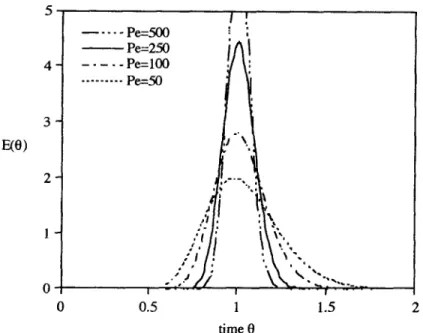
14 A. Pinheiro Torres, F: A. R. Oliveira 5 --____&-500 - Pe=2.50 4- ---.-pe=lOf) 0 0.5 1 1.5 2 time 8
Fig. 1. E-curves for different Peclet numbers, using the dispersion model.
is shown in Table 6 and the corresponding RTD curves are represented in Fig. 1, for different Pe numbers.
Wehner and Wilhelm (1956) solved analytically the differential equation resulting from a mass balance to a reactant in an axially dispersed plug flow reactor, which follows a first order kinetics, and obtained an expression for the final concentration as function of the kinetic rate parameter for the reaction and the Pe number (Levenspiel, 1972). This equation is valid for any kind of boundary conditions and can be rewritten as function of dimensionless numbers Pe and Da:
ce
i i
4ccepef2 - = f (Pe,Da) =
Ci (1 +a)2e%Pa’2 _ (1 _ x)*e _ xPe’2 (13)
with:
a = b: 1+4DalPe (14)
where the Damkohler number, Da, is a dimensionless form of expressing the reac- tion rate constant, k:
Da=kxs (15)
The N-CST model has also been applied to describe flow in tubes (Levenspiel & Bischoff, 1963; Wen & Fan, 1975) and in aseptic processes (Veerkamp et al., 1974; Roig et al., 1976; Wennerberg, 1986; Malcata, 1991; Sancho & Rao, 1992).
Residence time distribution studies IS
It is interesting to note that some stochastic non-ideal RTD models (single CST, DPF for large Pe and the N-CST) are equivalent to classical probabilistic models (exponential, normal and Poison distribution, respectively). These are also repre- sented in Table 6 for comparison.
Relating RTD parameters with product properties and processing conditions
Several correlations relating Pe to the Reynolds number (Re) were found in litera- ture for Newtonian fluids in tube flow (Table 7). One should note that those correlations are usually based on the axial Peclet number, Pe,,, which is related to the diameter and not the length of the tubular system:
(16)
No correlations were found for the transient regime. In laminar flow, the relation between Pe and Re is also dependent on the Schmidt (SC) number that relates hydrodynamic with diffusional mass transfer.
TABLE 7
Empirical Correlations Between RTD and Processing Parameters
Reference
Lcvenspiel (1958)
Wen and Fan (1975)
Correlation
Laminar flow: l/Pe,, = f(Re, SC)
I Rr x Sc --~ Pr,, - 192 I I Rex& -==+-t Pe;, Rr x Sc 192 Restrictions ___ He < 2 100 Re < 2000
Turbulent flow: l/Pet, = f(R,, Lid)
Taylor (1954)
Nassauer and Kessler (1979)
I 2.010 - - _* Pr, - Re” ‘15 I 0.766 -=- Pe;, Re” ’ Sjenitzer (195X) * Re > 3000 Re > 3000 Re > 3000
Wen and Fan ( 1975) I 3.0 x IO’ I.35 Re > 3000
p=
PC,, Re2.1 + Re” 125
*Altered using the Blasius equation, which relates the friction factor to the Re number (Bird
16 A. Pinheiro Torres, E A. R. Oliveira
Estimation of parameters from experimental data
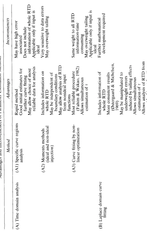
A full analysis of RTD curves requires an appropriate raw data treatment and the subsequent fitting of models to experimental data. Various methods can be applied to obtain the characteristic parameters of the RTD models and the techniques available for parameter estimation can be divided in time or Laplace domain analy- sis. The first is the most commonly adopted, either by using analysis of given characteristics of the RTD curve, moments analysis or curve fitting by non-linear optimization. Frequency domain curve fitting has also been described, although rarely used in aseptic processing. Advantages and inconveniences of these methods are summarized in Table 8. Some of the above mentioned methods allow the analysis of RTD curves obtained from non-ideal input functions.
‘Ikeatment of raw data of RTD curves
RTD curves may be obtained simply from normalization of output concentration curves to a Dirac input, according to eqn (1). The mean residence time (eqn (2)) can be directly calculated, as well as the variance, skewness and kurtosis (Table 1). To evaluate the integrals for moments calculation, the integration has to be done up to some finite time, and Aris (1959) reported that in order to guarantee an error lower that 1% in the estimates, integration should be conducted up to a time period equivalent to three times the mean residence time. If the first moment equals the mean holding time r, the RTD curves can be readily normalized with respect to time (eqn (6)); otherwise this parameter is preferably estimated together with the model curve parameters (Fahim & Wakao, 1982). As evaluation of moments is very influenced by data errors (noise, premature truncation of response or tailing of RTD curves), normalization of the RTD curves should be cautiously applied.
Tailing of RTD curves is commonly observed and several models have been put forward to explain this anomaly (Levenspiel, 1972). These models may be rather complex and with regard to application of RTD in the estimation of reactants’ conversion, the tail correction usually does not justify the extra modelling work (Levenspiel, 1972). On the other hand, the tailing assumes an important role in the accurate estimation of the model parameters, even in terms of the computation of the moments of RTD curve. Several solutions have been proposed in literature for overcoming this problem: (i) truncation of the output curve and approximation of the tail after the truncation point to an exponential decay (Wen & Fan, 1975); (ii) estimation of parameters from other sections of the RTD curve (Levenspiel, 1972); (iii) empirical corrections of RTD curves (Wen & Fan, 1975); and (iv) use of Laplace transform techniques which allow for linearization of the RTD curve (0stergaard & Michelsen, 1969; Hopkins et al., 1969).
Time domain curve analysis
The most simple and rapid method for parameter estimation in the time domain consists in analysing specific characteristics of the RTD curve (Al in Table 8) such as the peak time and height, inflection points or defined areas under the RTD curve. For example, Pe in the dispersion model can be estimated from the peak height of the E-curve, or N in the N-CST model can be estimated from the peak time (Levenspiel, 1972). Model parameters estimated in this way may not be very
TABLE 8 Advantages and Inconveniences of Parameter Estimation Methods Method Advantages Inconveniences (A) Time domain analysis (Al) Specific curve regions analysis (A2) Moments methods (ideal and non-ideal injection) (A3) Curve fitting by non- linear optimization (B) Laplace domain curve fitting Rapid method Good initial estimates for further curve fitting May allow choice of most reliable data for analysis May have high error associated Does not include information of whole RTD Applicable only if input is ideal Includes information on whole RTD May be independent of boundary conditions May allow analysis of RTD from nonideal input functions Most reliable procedure (Fahim & Wakao, 1982) Allows simultaneous estimation of T Very sensitive to data errors May overweight tailing Same weight to all RTD information-time consuming May overweight tailing Applicable only if input is ideal Includes information of whole RTD More consistent results \f.s;rgaard & Michelsen. May be manipulated to underweight errors induced by tailing effects Allows simultaneous estimation of T Allows analysis of RTD from non-ideal input functions Further mathematical development required
18 A. Pinheiro Torres, E A. R. Oliveira
accurate, but provide good initial estimates for further time domain curve fitting (Fahim & Wakao, 1982).
The moments of tracer curves (A2 in Table 8) may also be used to estimate directly the parameters of some simple models, such as the dispersion model for different boundary conditions (Levenspiel & Smith, 1957; Petho, 1968), in case of ideal tracer injection. For cases where the input tracer function is not ideal, Aris (1959) proposed a method for estimating dispersion numbers from moments analy- sis for both injection and response curves for open vessels. This method, corrected by Bischoff (1960) was extended to other experimental schemes with different boundary conditions applied to the dispersion model by Bischoff and Levenspiel (1962a), and is also described by Wen and Fan (1975). It consists in calculating Pe from the difference of variances of both input and output RTD responses, where
Ao2 = a: - a? = 21 Pe (17)
Levenspiel and Bischoff (1963) summarized the main advantages of this method for nonideal input functions: (i) it does not require any specific distribution of the input; (ii) it does not depend on the boundary conditions; (iii) it uses the information contained in the whole RTD curve, not only specific characteristics. The main drawback is that the estimated moments are greatly dependent on the tail end of the recorded curve, and therefore slight errors at higher times may be strongly magni- fied.
Time-domain curve fitting by non-linear optimization (A3 in Table 8) is con- sidered the most reliable procedure (Fahim & Wakao, 1982). The model parameters may be estimated by non-linear optimization techniques, although problems may arise when estimating simultaneously more than one parameter, particularly if they are highly correlated. Furthermore, mean residence time can be estimated along with the model parameters (Rangaiah & Krishnaswamy, 1990).
Laplace domain curve fitting
Other methods applicable to data processing of non-ideal pulse responses have been proposed (Wen & Fan, 1975). These methods (B in Table 8) use the system transfer function G(s) in eqn (9) calculated from the experimental RTD curve. Results are obtained directly from curve fit in the s-domain using the models’ transfer functions (Hopkins et al., 1969; Ostergaard & Michelsen, 1969) or from a modified moments analysis in the Laplace domain (Ostergaard & Michelsen, 1969).
The range of s values which gives least error in the predicted model parameters has to be evaluated case by case and may eliminate tailing effects in results (Hop- kins et al., 1969). 0stergaard * Michelsen (1969) estimated Pe numbers for the dispersed plug flow model from both the moments method in the time domain and by the transfer function (performing a linearization in the Laplace domain for parameters estimation), and found the latter to give more consistent results and to be rather insensitive to the duration of the recording period, in contrast to the moments analysis. They also introduced a modified moments analysis in the Laplace domain, which was the only method of nonideal input function analysis applied to RTD in an aseptic processing system (Kiesner and Reuter, 1988, 1990).
Residence time distribution studies IY
EXPERIMENTAL AND MODELLING STUDIES
Minimum holding times
Earlier studies were conducted to check the correct sizing of hold tubes in industrial equipment. The theory of residence times was first adopted for determining ster- ilization efficiency (eqn (11)) in holding tubes. This was incipiently done by Jordan et al. (1949) Jordan and March (1953) and Jordan and Holland (1953) in holding tubes, although their work was largely ignored by other researchers at that time (Lin, 1979). This kind of studies was later applied in the late 1960s on commercial equipment, as can be seen in Table 9. The main application of these studies was to check the correct sizing of hold tubes in industrial equipment.
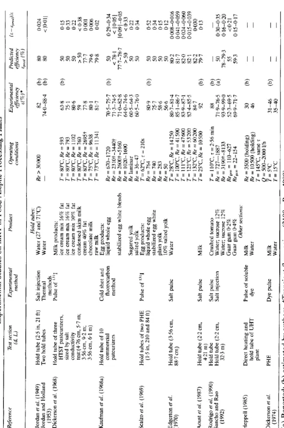
Table 9 summarizes the experimental methods and operating conditions for each case studied, including experimental efficiency values. When these values were not reported, we have estimated them from reported values of minimum and average holding time. Table 9 also includes efficiency values predicted using the adequate models presented in Table 4. In the cases where reported data was insufficient to describe the fluid rheological behaviour, we considered the conservative case of Newtonian fluids, as proposed by Dickerson et al. (1968) and Scalzo et al. (1969). It was found that experimental efficiencies are in general greater than those predicted. which may be due to three main reasons: (i) nonideality of the flow - this may be significant in situations where laminar flow is not fully developed, or when the fluid is flowing through bent pipes, so that streamlines are broken, inducing a higher mixing of fluid, less spread of residence times and higher mRT; (ii) sensitivity of the tracer detection method - the higher the tracer quantity required for detection, the lower the efficiency value experimentally determined (Jordan et al., 1949; Jordan & Holland, 1953); and (iii) errors in the calculation of the mean residence time. The only exception, where predicted efficiencies were greater than those measured experimentally, was found for some egg products in the transition flow regime (Kaufman et uf., 1968a), but in this study Re numbers were calculated assuming Newtonian flow behaviour, not taking into consideration that many egg products may show a pseudoplastic flow behaviour and/or yield stress (Holdsworth, 1971; Rao, 1977; Steffe, 1992). This comment is also valid for the work of Dickerson et ul. (1968) who studied some milk products (condensed skim milk, cream with 40% fat) and for the work of Rodrigo et al. (1990) on crushed tomato. Relative deviations between experimental and predicted efficiencies for most Newtonian fluids (water and some milk products), were found to be positive and relatively low, while dependant on flow regime ( < 2.4% for turbulent, < 5% for transient and < 22% for laminar flow). On the other hand, relative deviations for egg products showing Newtonian flow behaviour (up to 52%) reported by Kaufman et al. (1968a) and Scalzo et al. (1969), were much larger, suggesting that the tracers used in egg products may have a quite different detection level.
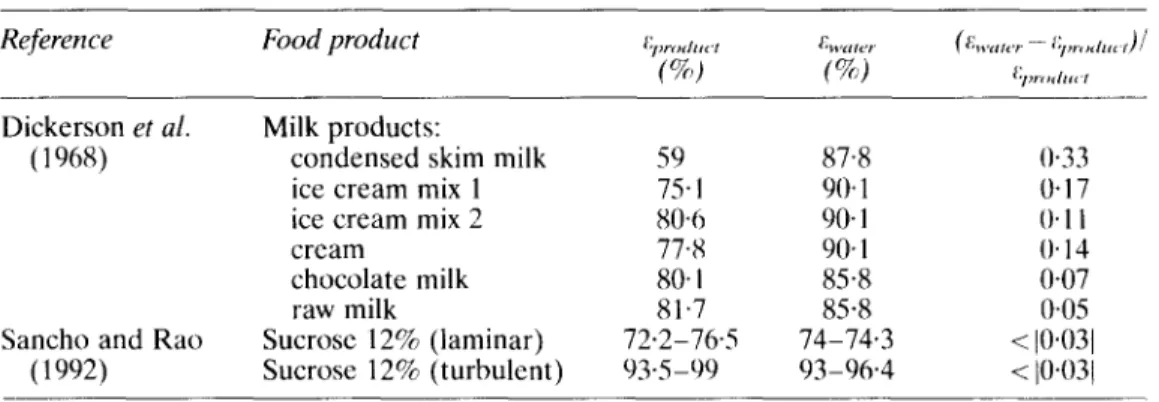
In many situations, efficiencies are experimentally assessed by the standard salt conductivity test performed on water, at processing conditions (holding time and temperature) identical to those the real food product will be subjected to. It is therefore most important to assess the validity of such procedure. We have cal- culated relative deviations between experimental efficiencies of water and other food products from published data (Table 10). Deviations up to 3% (Sancho & Rao, 1992) and 7% (Dickerson et al., 1968) were found for Newtonian fluids, indepen-
TABLE 9 Experimental Studies on mRT in Food Aseptic Processing Plants (8 - $,,,)lC Reference Test section Experimental (d, L) method Producr Operating conditions Experimental Predicted ejjkiency eficiency s(s)* &Ll f%%) Jordan er al. (1949) Jordan and Holland (1953) Dickerson et al. (1968) Hold tubes: Water (27 and 71°C) Water 80 80 T = 8O”C, Re = 593 63.8 T = 80°C. Re = 793 75.1 T= SO”C, Re = 1102 80.6 T = 80°C. Re = 760 T = SOT, Re = 2695t 59 77.8 T = 75”C, Re = 9638 80.1 T=73”C,Re=11341 81.7 (b)
2:
50 z 50 77.7 796 79.8 70.5-75.7 (b) 50 71.3-745 < 78. I 7 1 .o-82.8 77~7-78.7 64.0-74.6 >50 605-64.3 50 60,5-76.0 50 80.9 (b) 75.7 58.6 56.6 80.7-81.4 85.1-86-7 83.9-87.1 83.4-855 84.7 92 (b) $8;;:; ii] 52.3-69.5 69.9-71.7 50 :: 50 80.2 81.7 82.0 82,l 82.2 79.1 30 (h) 46 31-46 35-40 (b) 50 78-79.3 55 59-3 - - - 0,024 < IO.011 Hold tube (2.5 in, Two hold tubes 21 ft) Salt injection Thermal methods Pulse of “‘I Re > 30000 Hold tube of three HTST pasteurizers, sized bv salt conduciivity test:(4.76 cm, 5.7 m; 3,S6 cm, 9.2 m; 3.56 cm, 6-l m) Milk products: ice cream mix 16% fat ice cream mix 16% fat ice cream mix 10% fat condensed skim milk cream 40% fat chocolate milk raw milk Egg products: liquid whole egg stabilized egg white blends 0.15 0.33 0.22 Hold tube of 10 Cold shot and commercial fluorocarbon pateurizers method -=z 0.38 O+Ol 0.006 0.02 0.29-0.34 ( IO.051 ) “‘“,“A;? 0.22 0.34 0.52 0.34 o-15 0.12 O+NX-0.016 0.04 l-0-059 0.024-0.060 0.0 15 -0.039 Kaufman et al. (1968a) Re = 670-1720 Re = 2310t-3440t Re = 26OOt-5 160 Re = 1020-1600 Re laminar Re = 36-47 T=62”C,r=ZlOs Re = 764 Re = 740 Re = 283 Re = 50 T = 28”C, Re = 14250 T = lOO”C, Re = 41500 T=lll”C,Re=47600 T = 121”C, Re = 53 200 T = 132”C, Re = 60200 T = 25”C, Re = 10.500 Sugared yolk salted yolk Egg products: liquid whole egg stabilized egg white plain yoIk 10% salted volk Scalzo ef al. (1969) Hold tubes of two PHE (I.5 in, 210 and 84 ft) Pulse of 13’1 Edgerton et al. Hold tube (3.56 cm, (1970) 88.7 cm) Salt pulse Water 0.030 0.13 Aoust et al. (1987) Hold tube (2.2 cm, 421 m) Hold tube Hold tube (2.2 cm, 32.3 m) Salt pulse Milk Salt pulse Salt injection Crushed tomato Water; sucrose 12% Water; sucrose 12% Guar gum 0.2% Guar gum 0.4% Other sections. Milk Water Rodrigo et al. (1990) Sancho and Rao (1992) T = I lO”C, T = 256 min Re = 727-1887 0.30-0.35 0.16-0.20 to.21 0.15-O-17 ;; = 319ot-8133 - 110-627 Rez:l= 22-154 Heppell (1985) Direct heating and hold tube of UHT plant Pulse of soluble dye PHE Dye pulse Re = 3500 (holding) Re = 10500 (holding) T = 145°C. same z Dickerson et al. (1974) Milk Water - (a) Reported; Cb) estimated bv authors. tTransient flow regime 12100 < Re <41)1)O\.Residence time distribution studies 21
TABLE 10
Comparison Between Experimental Efficiencies for Water and Food Products
Dickerson et al. ( 1968)
Sancho and Rao ( 1992) _
Milk products:
condensed skim milk
ice cream mix 1
ice cream mix 2
cream chocolate milk raw milk Sucrose 12% (laminar) Sucrose 12% (turbulent) 59 87.8 0.33 75.1 90.1 @I7 80.0 90.1 0.1 I 77.8 90.1 0.14 80. I 85.8 0.07 81.7 85.8 0.05 72.2-76.5 74-74.3 < 10.031 93.5-49 93-96.4 < 1O.U
dently of the flow regime. Non-Newtonian fluids show much higher deviations, as would be expected, reaching values as high as 33%. Dickerson et al. (1968) found that the standard salt conductivity test was satisfactory for milk and chocolate milk, whereas errors up to 33% were found for more viscous milk products. Heppell
(1985) also compared mRT values obtained for water and for milk processed in a heat and a holding section of a UHT plant, for three different holding temperatures. To maintain the same temperature and mean residence time, for water and milk, different flow rates and thus different Re numbers were however used for each fluid, thus preventing a true comparison from being made. Similarly, Dickerson et al. (1974) compared efficiencies for milk and water in a PHE, but using different processing temperatures for each product.
In general terms, it should be stressed that there are various sources of errors that should be carefully taken into consideration when determining both mRT and efficiency values in continuous processing systems. The models proposed in Table 4 appear to be conservative when applied for hold tube sizing, thus guaranteeing the product safety, except for products flowing in the transition zone (2100 < Re < 4000). The classical test of salt conductivity in water yields good results for Newtonian fluids, but is quite conservative when applied for non-Newtonian fluids.
Residence time distributions
Table 11 summarizes reported experimental studies on RTD in holding tubes of food aseptic processing plants. Similar information for heat transfer sections (heat- ing and cooling) can be found in Table 12. Most studies were conducted with water and salt was preferred as tracer. Model food products tested include sucrose and guar gum solutions (Sancho & Rao, 1992) diethylene glycol (Pudgiono et al., 1992) polyethylene glycol (Milton & Zahradnik, 1973), glycerol-water mixtures (Tromme- len & Beek, 1971) and starch (Bateson, 1971). RTD studies on real products were performed with milk (Cerf & Hermier, 1973; Nassauer & Kessler, 1979; Heppell, 1985; Janssen, 1994) and coffee cream (Kiesner & Reuter, 1988).
The first RTD studies in holding tubes (Table 11) were performed by Jordan and March (1953) and Dickerson et al. (1968), to assess overholding times (holding
22 A. Pinheiro Ton-es, l! A. R. Oliveira
times expressed in a shifted time scale where mRT is taken as time zero) and their dependence on processing conditions. One can find studies on a large diversity of holding tubes sizes although a limited number of processing conditions was tested for each. Jordan and March (1953), Burton (1958a), Chen and Zahradnik (1967), Milton and Zahradnik (1973), Burton et al. (1977) and Janssen (1994) were the only authors that tested RTD in holding tubes at temperatures above ambient. Studies
TABLE 11
Experimental Studies on RTD in Food Aseptic Processing Plants - Hold or Straight Tubes
Reference Test section
cd, L)
Method Product No. of
runs Operating conditions Jordan and March (1953) Burton (1958a) Aiba and Sonoyama (1965) Chen and Zahradnik (1967) Milton and Zahradnik (1973) Veerkamp et al. (1974) Roig et al. (1976) Burton et al. (1977) Nassauer and Kessler (1979) Wennerberg (1986) Kiesner and Reuter (1990) Sancho and Rao (1992) Janssen (1994) Hold tubes (l-2.5 in; 9-53 ft) Hold tube of PHE
Salt pulse
Straight tubes
(3.9 mm, 2.37+ 11 m) Hold tube of SSHE
Sodium nitrite Step of ‘*P marked microbial suspension Sucrose pulse
Hold tube of SSHE Sucrose pulse
Two hold tubes, same T (8 cm, 1.5 m) (1.35 cm, 52.5 m) Two hold tubes
Hold tube (<25mm, <52m) (35.6 mm, 43.3 m) (65 mm, 15.3 m) (5.0 cm; 1.05 m) (2.22 cm, 32.3 m) Hold tube (7 = 70s) Salt pulse
Dye step and purge Salt pulse Salt step Salt pulse Salt pulse Salt pulse Salt Water Water Water Water PEG* 25% Water Water Water Water Milk Water Water Water Sucrose 12% Guar 0.2 and 0.4% Milk 9 1 2+1 3 2 2 2 1+5 1 1 2 12 10 10 7+5 1 Re = 7500-50000, T = 71°C Re = 25000; T = 135°C Re = 420 and 2260 Talllh Three flowrates, T=87”C Two flowrates, T = 124°C T&, 5 = 140 s, Re = 860, Re=5100 Two flowrates, T = 26.7”C; T = 9-13.3 s Re > 5000; T = 130-150°C Re = 5000 Re = 5820; Tamh Re = 21400,35 300; Tnmh Re = 20 000-100000 Re = BOO-8133 Re = 727-6071 Regen = 22-627 T = 25°C T=90”C *Polyethylene glycol.
Residence time distribution studies TABLE 12
23
Experimental Studies on RTD in Food Aseptic Processing Plants-Heating and/or Cooling
Sections PHEs Watson rt al. (1960) Wennerherg (1986) Kiesner and Reuter (198X) Burton (lYS8a.b) Direct HEs Serf and Hermier (1973) Heppell (1985) SSHES Batcson ( 1 Y7 I ) C‘hcn and Zahradnik (1067) Trommclen and Beek (1071) Milton and Zahradnik ( lY73) c‘ucws r’l al. (10X2) Ahichandani and Sarma ( 10x8)
3 PHE Salt and dye step
PHE (two arrangements) PHE (four arrangements) Salt pulse Salt pulse, nonideal PHE. heat Steam injection Direct heating and hold tuhe of UHT plant 3 SSHE 2 SSHE (one heating and one cooling section) SSHE 2 SSHE (one heating and one cooling section) Vertical SSHE Horizontal thin film SSHE Vertical SSHE Sodium nitrite pllW Dye pulse Pulse of soluhlt dye Salt pulse hOci sucrcjse pulse Dye pulse Dye \tep Salt pulse Dye pulse Water Water Water (‘offee cream Water Milk Water Water Starch S!i Water Glicerob water mixtures PEG 25? Water Water water DEG s+2 60 I - I 1 I I I7 5 s 36 T constant Rr = 25 000, T = 135°C T= 102-l I%:, Q = I.9 limin Kc = 3500 and 10 500 (only in holding tube) T = 13X- 147°C. same (3+ l+ I) fowrates (3+ I + 1) rotor speeds T constant
each: three tlowrates. four rotor speeds
AT = 70-X7”<‘ Same Howrate, two
How regimes. four rotor speeds each: two Howrates.
four rotor speed\
AT = 4% 121°C
T = 130°C
I I #(32 trials) Three Howrates. three
rotor speeds. four blades. T .,,,,,,
2 L\.,lCl = 0~7-0~34, tw1,
rotor speeds
7 r,>,.<;_ = 544x2s;
T = 20°C‘ 2Q. five rotor speeds
24 A. Pinheiro Torres, I? A. R. Oliveira
on heating and cooling sections of aseptic processing plants (Table 12) were per- formed on PHEs, SSHEs and direct heating systems.
Eventual tailing effects in RTD curves should be carefully assessed. Tailing effects are masked in RTD curves obtained from a step injection of tracer. In most of the reported RTD curves obtained from a pulse injection of tracer in a holding tube, a significant tailing in RTD could be observed. Tailing effects may arise from improper injection (Milton & Zahradnik, 1973) or indicate laminar or low turbulent flow regimes. Except for the work of Burton (1958a), negligible tailing was found for
Re numbers above 20000. These effects are in general overlooked in the modelling of RTD curves.
Modelling of RTD curves in holding tubes is quite common, while only four works were found reporting modelling of RTD curves obtained in heating systems (Table 13). Models presented include (i) the velocity distribution model; (ii) the N- CST model, with or without PF in series; and (iii) the dispersed plug flow model. These models were based on the assumption of ideal injection of tracer, with the
TABLE 13
Models Proposed for Experimental RTD Curves
Reference Relproduct Model (parameters)
Straight or hold tubes Aiba and Sonoyama (1965)
Veerkamp et al. (1974)
Roig et al. (1976)
Burton et al. (1977)
Nassauer and Kessler (1979)
Wennerberg (1986)
Sancho and Rao (1992)
PHE’s
Wennerberg (1986)
Kiesner and Reuter (1990)
SSHEs Bateson (1971) Pudgiono et al. (1992) 420lwater 22601water 860lwater 5 1 OO/water -/water -/water 5000/water 5820/milk 21400iwater 35 300/water
BOO-8133/water and sucrose 12%
11 O-627lguar 0.2%
22-154/guar 0.4%
(21400 and 35300 in hold)/ water
500-8000lwater and coffee
cream
(3+ 1+ 1) flowrates, (3 + 1 + 1)rotor speeds/ water
Several fiowrates, and rotors peeds/water and DEG
Velocity distribution DPF (Pe = 320) PF+2.3 CST PF+7 CST N-CST (N = 5) and F = 11 exp( Lath) PF Velocity distribution DPF+velocity distribution N-CST (N = 340) DPF (Pe = 4100) N-CST and DPF (N = 14-103, Pe, = 0.02- 0.17) (N = 18-34, Pe, = 0.01-0.05) (N = 7-12, Pe, = 0.01-0.05) 5-CST and 2 DPF DPF ‘between PF and CST’ DPF
Residerzce time distribution studies 2s exception of the work of Kiesner and Reuter (1988). Model parameters were some- times estimated by fitting the whole RTD curve to the model; alternatively, parameter estimation was based on statistical analysis, namely from the variance of RTD curves. As earlier referred, the latter procedure may lead to inaccurate esti- mates if tailing effects occur. In many cases curve fitting and data treatment is not very clear; the goodness of fit between experimental and predicted RTD was never quantified. Results reported by different authors for similar processing systems and conditions (Re number) are often quite different, thus making difficult to find general conclusions.
Application of RTD curves for process optimization is uncommon (Pinheiro- Torres & Oliveira, 1994). RTD curves were applied to estimate final concentrations of surviving microorganisms only in a few cases (Bateson, 1971; Burton, 1958b; Burton ct al., 1958, 1977; Milton & Zahradnik, 1973; Veerkamp et al., 1974; Wen- nerberg, 1986).
Relating mRT and RTD to processing conditions
Some authors studied the effects of processing conditions on holding tube effi- ciencies: Scalzo et al. (1969) found a decrease of mRT (and thus hold tube efficiency) with product viscosity, for a number of egg products. Dickerson et 171.
(1968) concluded that mRT is related to tube diameter, tube length and number of bends and to the viscosity of the different milk products. Edgerton et al. (1970) studied the effect of pressure and temperature on the product maximum velocity in a hold tube. Experimental mRT values were higher than predicted values and this deviation increased with the Reynolds number. Jordan and March (1953) studied the effects of tube length, tube diameter and fluid velocity (water) on overholding time, concluding that overholding time decreases with velocity (for constant tube diameter) and increases with diameter (for constant velocity).
Analysis of the effect of processing conditions on RTD in SSHEs, was qualita- tively reviewed by Singh and Lee (1992). Chen and Zahradnik (1967) and Milton and Zahradnik (1973) studied the effect of flow rate, as well as rotor speed in the latter work, on the shape of RTD curves, concluding that an increase in these parameters has a narrowing effect on RTD curves. Abichandani and Sarma (1988) confirmed these results and found that an increased number of blades would narrow the RTD.
Analysis of the effect of processing conditions in the RTD of holding tubes is scarce. Sancho and Rao (1992) found that the Pe number was lower for laminar than for turbulent flow, independently of the type of the liquid tested, but no clear correlation between Pe and Re numbers could be found.
CONCLUSIONS
The knowledge of mRT is essential for sizing holding tubes. This processing time may he measured experimentally or calculated from theoretical models, that were found to yield in general conservative estimates. Experimental methods for measur- ing mRT are well described in literature and several types of tracers were proposed for different types of liquid foods. These methods should be carefully applied to provide good results.
A. Pinheiro Torres, E A. R. Oliveira
There is a reasonable number of published RTD studies, but there is a clear need for a systematic approach and modelling studies. RTD determinations have been mostly conducted in test rigs, at ambient temperatures and the potential of RTD for optimization studies has not been fully explored.
Several model fluids have been used for RTD studies, covering a wide range of Newtonian and pseudoplastic flow behaviour. Water has been the preferred model fluid but its applicability is quite limited when simulating real fluid foods. Fluids showing very high viscosity or yield stress have not been tested yet in spite of their evident importance in aseptic processing, e.g. for simulating some milk or egg products, sauces or purees. Furthermore, model fluids able to withstand higher temperatures (typical in aseptic processes) have not been considered yet. Studies on real food products are very limited. If RTD experiments are to be extended to these products, tracers should be carefully selected. The tracers commonly applied in real food products are in general only suitable for mRT determinations, but can be used as a start point to new developments, provided their detection methods can be improved.
Relating RTD to processing conditions in aseptic processes is quite incipient and should be developed. These studies would provide an invaluable insight in the flow behaviour as has been widely recognized in the chemical engineering field.
ACKNOWLEDGEMENTS
The first author acknowledges Junta National de Investigaccao Cientifica e Tecnolo- gica (JNICT) for financial support under the scope of ‘Programa Ciencia’ and ‘Programa Praxis XXI’.
REFERENCES
Abichandani, H. & Sarma, S. C. (1988). Residence time distribution in a horizontal thin film
scraped surface heat exchanger (SSHE). Journal of Food Process Engineering, 10, 17-80.
Aiba, S. & Sonoyama, T. (1965). Residence-time distribution of a microbial suspension in a
straight pipe. Journal of Fermentation Technology, 43, 534-540.
Anonymous, (1950). Standard method for determining the holding time of HTST pasteur-
izers by means of the salt conductivity test. Journal of Milk and Food Technology, 13,
261-265.
Aoust, J.-Y. d’, Emmons, D. B., McKellar, R., Timbers, G. E., Todd, E. C. D., Sewell, A. M.
& Warburton, D. W. (1987). Thermal innactivation of salmonella species in fluid milk.
Journal of Food Protection, 50(6), 464-501.
Aris, R. (1959). Notes on the diffusion-type model for longitudinal mixing in flow. Chemical
Engineering Science, 9, 266-267.
Bailey, J. E. & Ollis, D. F. (1986). Biochemical Engineering Fundamentals, 2nd edn, McGraw
Hill, New York, Chap. 9.
Bateson, R. N. (1971). The effect of age distribution on aseptic processing. Chemical
Engineering Progress Symposium Series, 108(67), 44-52.
Bird, R. B., Stewart, W. E. & Lightfoot, E. N. (1960). Transport Phenomena, Wiley, New