Customized Hardware for Long-Short Term Memory Networks in Embedded Systems

F

E

U

P

Customized Hardware for Long-Short

Term Memory Networks in Embedded

Systems

Pedro Manuel Afonso Costa

Mestrado Integrado em Engenharia Eletrotécnica e de Computadores Supervisor: João Canas Ferreira

Resumo

Redes neurais do tipo Long Short-Term Memory (LSTM) têm sido aplamente usadas nos últimos anos, cuja implementação se tem dado em diversos campos, tais como reconhecimento de fala ou descodificação de gestos em teclado. Adicionalmente, tem-se verificado uma necessidade cres-cente de implementar LSTMs em ambientes de baixa potência, nos quais ASICs e FPGAs revelam ser as melhores soluções.

Paralelamente, tem-se assistido a notáveis desenvolvimentos no que toca às plataformas de de-senvolvimento em Síntese de Alto Nível (HLS), conduzindo a melhores resultados no que toca às descrições de Register Transfer Level (RTL). Por este motivo, as plataformas de HLS são cada vez mais consideradas uma alternativa viável a descrições em Linguagens de Descrição de Hardware (HDL), visto ter-se tornado possível a obtenção de circuitos de qualidade, ao mesmo tempo que são aproveitadas as vantagens resultantes da utilização de linguagens de alto nível, nomeadamente o menor esforço de implementação.

Considerando os aspectos acima, este trabalho propõe o desenvolvimento de uma rede LSTM para uma plataforma FPGA, com recurso a ferramentas HLS. Devido à dimensão elevada das redes LSTM comparativamente com a memória interna de uma FPGA, é proposto o armazenamento dos pares de entrada e dos pesos da rede em memória externa. Para evitar as elevadas latências associadas à utilização exclusiva de memória externa, é proposta uma técnica do tipo “block-batching”, a qual permite efectuar operações sobre um conjunto de pares de entrada e um bloco de matrizes de pesos, os quais são transferidos de memória externa para memória interna através de “double-buffering”. Por forma a obter um maior nível de paralelismo, bem como a reutilização dos elementos instanciados na FPGA, a implementação dos blocos com maiores necessidades computacionais recorre à utilização de pipelines. É também possível variar a topologia da rede instanciada através de um conjunto de parâmetros. A dimensão em bits de cada word pode ser ajustada de acordo com as necessidades do sistema.

Aquando da utilização do dataset MNIST, a arquitectura proposta utiliza uma menor dimensão de word para as suas variáveis, a qual resulta numa redução dos requisitos de memória interna até 1.14x comparativamente a trabalhos anteriores, incorrendo num aumento do erro de até 2.2%. Após implementação do acelerador proposto numa placa física, melhorias de 1.99x e 10.53x na velocidade de execução são registadas comparativamente a processadores desktop e embedded, respectivamente.

Palavras-chave: FPGA, HLS, LSTM, Redes Neuronais

Abstract

Long Short-Term Memory (LSTM) neural networks have been widely used in recent years, being deployed in a range of scenarios such as speech recognition or keyboard gesture decoding. In addition to this, there is an increasing necessity of implementing LSTMs in environments with low power budgets, for which ASICs and FPGAs are the most sensible solutions.

Parallel to this, High-Level Synthesis (HLS) development platforms have markedly improved in recent years, resulting in better Register Transfer Level (RTL) descriptions. HLS is then increas-ingly seen as a feasible alternative to Hardware Description Language (HDL) descriptions, as it is now possible to obtain quality circuits with the advantages that derive from using higher-level programming languages, namely its lower implementation effort.

Considering this, the present work proposes the development of an LSTM network for an FPGA platform using HLS tools. Because of the large size of LSTM networks in comparison with the on-chip memory available in an FPGA, off-chip memory storage of the input pairs and the weight matrices is proposed. To avoid dealing with large latencies derived from exclusively using off-chip memory, a block-batching technique is presented, which performs computations over a batch of input pairs, and a block of weight matrices, which are buffered from off-chip into the on-chip memory using double-buffers. For obtaining a higher level of parallelism and the reuse of the elements instantiated on fabric, the implementation of the most computationally-intensive blocks is performed using pipelines. Furthermore, it is possible to vary the topology of the network by using a number of parameters for that purpose. The word bit-widths can also be adjusted according to the needs of the system.

When using the MNIST dataset, the proposed architecture uses a smaller word bit-width, re-sulting in a reduction of up to 1.14x of on-chip memory requirements in comparison with previous works, while incurring a maximum error of up to 2.2%. After implementing the proposed acceler-ator on a board model, speed-ups of 1.99x and 10.53x are registered, respectively, in comparison with a desktop and an embedded CPU.

Keywords: FPGA, HLS, LSTM, Neural Networks

Agradecimentos

Gostaria de agradecer a todos os professores com quem me cruzei durante o meu percurso académico, sem os quais não seria possível a minha formação, nomeadamente os desta Facul-dade de Engenharia. Agradeço também ao Prof. João Canas Ferreira pela proposta que realizou, e por ter colocado, através da sua orientação, a sua experiência ao meu serviço.

Agradeço também o apoio dos meus amigos durante as várias fases da minha vida, e das inúmeras pessoas com que me cruzei e que me ajudaram durante o curso. Agradeço também aos meus colegas de quarto durante o meu intercâmbio em Delft, Holanda, pelo que me ensinaram sobre tolerância e sobre manter a vida em perspectiva.

Os meus agradecimentos não estariam completos sem mencionar a minha família mais próx-ima. Aos meus pais, e à minha avó, agradeço-lhes o seu amor incondicional e o apoio incansável, com o qual pude contar quando mais necessitei. Ao meu irmão, agradeço-lhe a sua boa-vontade em ajudar-me durante o meu percurso, e a sua orientação inestimável.

Pedro Manuel Afonso Costa

“Stay hungry, stay foolish.”

Steve Jobs

Contents

2.2 Artificial Neural Networks . . . 4

2.2.1 Perceptron . . . 4

2.2.2 Activation Functions . . . 5

2.2.3 Forming ANNs . . . 6

2.2.4 Training . . . 7

2.3 Recurrent Neural Networks . . . 8

2.3.1 Overview . . . 8

2.3.2 Long Short-Term Memory Networks . . . 10

2.4 High Level Synthesis . . . 11

2.4.1 Overview . . . 11

2.4.2 Pragmas . . . 12

2.4.3 Data Types . . . 15

2.5 Summary . . . 16

3 State of the Art 17 3.1 LSTM Applications: Overview . . . 17 3.2 LSTM Implementations on FPGA . . . 18 3.3 Summary . . . 21 4 Proposed Architecture 23 4.1 Overview . . . 23 4.1.1 Description . . . 23 4.1.2 Matrix computations . . . 25 4.1.3 Fixed-Point Design . . . 27 4.1.4 Coding Structure . . . 27 4.2 Constituent Modules . . . 28 4.2.1 Initialisation . . . 28 4.2.2 Buffering Blocks . . . 28 4.2.3 Computation Blocks . . . 29 4.2.4 Auxiliary Blocks . . . 32 ix

x CONTENTS 4.3 Summary . . . 34 5 Results 35 5.1 Simulation Validation . . . 35 5.2 Synthesis Results . . . 36 5.3 Accuracy Measurements . . . 38 5.3.1 Overview . . . 38 5.3.2 Training . . . 38 5.3.3 Results . . . 38 5.4 Board Implementation . . . 40 5.4.1 Overview . . . 40 5.4.2 Results . . . 42 5.4.3 Comparison . . . 43 6 Conclusions 47

A Network Training in PyTorch 49

B Resource Utilisation Results 55

List of Figures

2.1 A perceptron . . . 5

2.2 Examples of activation functions . . . 6

2.3 An ANN with three connected layers . . . 7

2.4 An RNN and its unrolled equivalent . . . 8

2.5 An LSTM cell . . . 10

2.6 Array transformations . . . 13

2.7 Loop pipelining . . . 15

4.1 High-level architecture of the LSTM accelerator . . . 24

4.2 Matrix traversal used in the block-batching technique . . . 26

4.3 Architecture of the 4-LFSR GPRNG . . . 33

4.4 Architecture of the PLAN algorithm . . . 33

4.5 Comparison of the original functions with PLAN . . . 34

5.1 Impact of Sbatchand Sblockfor the simulated accelerator . . . 37

5.2 Network accuracy for the MNIST training set with respect to the number of train-ing epochs and the <W,I> pairs . . . 39

5.3 Network accuracy for the MNIST training set with respect to the word bit-width <W> of the input pairs . . . 40

5.4 Block design for implementing the proposed accelerator on the VC707 board . . 41

5.5 Impact of Sbatchand Sblockon the board implementation . . . 43

C.1 C/RTL Cosimulation output waveforms . . . 57

List of Tables

3.1 Summary of the described LSTM implementations on FPGA . . . 21

5.1 Network parameters used for studying the effects of block-batching . . . 36

5.2 Resource utilisation results for the simulated accelerator . . . 37

5.3 Network accuracy for the MNIST training set . . . 39

5.4 Resource utilisation results for the board implementation . . . 43

5.5 Performance comparison against CPU implementations . . . 44

5.6 Comparison against previous works . . . 44

B.1 Latency and resource utilisation results for the simulated accelerator . . . 55

B.2 Latency and resource utilisation results for the board implementation . . . 56

Abbreviations

ASIC Application-Specific Integrated Circuit AXI Advanced eXtensible Interface

BRAM Block RAM

CORDIC COordinate Rotation DIgital Computer CPU Central Processing Unit

CUDA Compute Unified Device Architecture DSP Digital Signal Processor

FF Flip-Flop

FPGA Field-Programmable Gate Array GOP/S Giga Operations per Second GPRNG Gaussian PRNG

GPU Graphics Processing Unit HDL Hardware Description Language HLS High Level Synthesis

IC Integrated Circuit II Initiation Interval I/O Input/Output IP Intellectual Property JTAG Joint Test Action Group LFSR Linear Feedback Shift Register LSTM Long-Short Term Memory LUT Look-Up Table

ML Machine Learning

PLAN Piecewise Linear Approximation PRNG Pseudo-Random Number Generator RAM Random Access Memory

RNN Recurrent Neural Network RTL Register Transfer Level

SIMD Single Instruction, Multiple Data SoC System-on-a-Chip

VHDL Very High Speed Integrated Circuit HDL

Chapter 1

Introduction

In this work, a hardware implementation of an LSTM network is presented. This accelerator is implemented on an FPGA and designed for manipulating large networks. For the purpose, a block-batching technique and off-chip memory storage are used. This accelerator also allows the manipulation of the internal bit-widths which, for the MNIST dataset, results in a reduction in memory requirements of up to 1.14x in comparison with previous works. After implementation on a board model, speed-ups of 1.99x and 10.53x are registered upon comparison with a desktop and an embedded CPU, respectively.

1.1

Background

Long Short-Term Networks are a popular type of Recurrent Neural Networks. Introduced by Hochreiter and Schmidhüber in 1997, LSTMs are a state-of-the-art algorithm for capturing se-quences and time-series, using for that purpose a memory controller that retains long-term depen-dencies. As a result, LSTMs are now used in a wide range of applications on different types of hardware, from speech recognition algorithms to keyboard gesture decoders.

LSTM networks have been implemented in various computation environments. Notably, sev-eral CPU and GPU implementations are available, which are suitable for computing huge amounts of data with good performance. However, other approaches are needed when facing power con-straints. In this regard, solutions using ASICs or FPGAs can be helpful for implementing LSTMs due to their good power-performance balance. Specifically, FPGAs can be reprogrammed, thus opening up the possibility of altering the system on-the-fly.

Parallel to this, HLS software has registered notable improvements in recent years, to the extent that it is now a feasible platform to produce fast, efficient circuits. With it, the use of C/C++, along many of its useful features, is supported for describing hardware. One example is the ability of using templates, that enable rapid generation of different functions on hardware by altering some parameters. Additionally, using the included pragmas, the programmer can perform

2 Introduction

fine-tuning over some characteristics of the hardware, which would not be possible using high-level programming languages alone.

1.2

Motivation

Presently, a number of LSTM implementations on FPGA exist. Usually, the proposals focus on inference, and perform either data compression techniques or architectural improvements. Com-pression techniques have the advantage of reducing the size of the network (which translates to lower memory and computational requirements), and usually consist of some sort of pruning tech-nique performed to the weight matrices of the LSTM, while in other cases quantisation techtech-niques are mentioned. Architectural improvements may consist of buffering or batching techniques, and in some cases of alternative algorithms to compute the outputs of the LSTM.

However, most implementations do not enable rapid, effortless synthesis of different LSTM networks depending on the needs of the system. To enable this, the architecture needs to be able to accept a number of inputs that can be used to vary the topology of the network. Furthermore, and to the best of our knowledge, the only existing parametrisable implementation makes exclusive use of on-chip memory for storing all variables, which severely limits the dimension of the networks that can be processed.

1.3

Objective

In this work, the implementation of an LSTM network on an FPGA is proposed. For this purpose, a parametrisable accelerator is presented, which is implemented in Vivado HLS. The proposed accelerator uses a block-batching technique that buffers values from off-chip memory, and enables both effortless network topology changes and tuning of the word bit-widths of the variables. The proposed accelerator is implemented and tested on a board model.

1.4

Overview

The document is organised as follows.Chapter 2introduces the concept of Machine Learning and the theoretical considerations behind ANNs, with special focus on LSTMs, and the topic of High Level Synthesis.Chapter 3provides an overview of previous LSTM implementations in different research fields, and presents the state of the art in regard to implementations on FPGA.Chapter 4 presents the architecture of the accelerator proposed in this work, and describes its constituent blocks.Chapter 5presents the obtained results.

Chapter 2

Problem Characterisation

This section introduces and characterises the main topics to be covered in this work. Section 2.1 provides a general overview of Machine Learning and its concepts. Section 2.2briefly describes Artificial Neural Networks, from their basic building blocks to the necessary training procedures. Section 2.3delves into Recurrent Neural Networks, a specific type of ANN, and introduces the Long Short-Term Networks that are used in this work. Section 2.4 finishes by providing an overview of High Level Synthesis hardware description, which will be used to specify the RTL implementation to be synthesised on FPGA.

2.1

Machine Learning: Overview

Machine Learning (ML) is a research field of Computer Science that uses statistics and artificial intelligence to enable computer systems to learn and improve from experience without being ex-plicitly programmed [1]. This allows ML to extract latent features from the data, and enabling its classification into a particular class by using an adaptive model that adjusts its parameters accord-ing to the input data received.

Adopting ML solutions is useful in situations where hard-coded, rule-based algorithms may fail or be too cumbersome, such as in situations where small changes in a task require significant modifications to the code, or where defining rules would require a deep understanding of the subject. As a result, several ML algorithms have been developed, and most can be split into the categories below.

Supervised Learning

Supervised learning algorithms are able to automate decision-making processes by generalising from known samples. To achieve this, the algorithm is trained with pairs of inputs, or targets, and desired outputs, or labels, which constitute the training set and are used by the algorithm so that it finds a way to reproduce the input and output pairs. After the aforementioned training,

4 Problem Characterisation

the algorithm is able to produce an output, given a new input, without human intervention. These algorithms are usually the easiest to understand and evaluate.

A typical supervised learning task is classification, which provides an output corresponding to a discrete number of solutions, of which spam e-mail classification (i.e. spam or not spam) is an example [2]. Another typical task is regression, where a target value in a continuous range is inferred by using predictors, of which house pricing prediction (i.e. the value of a house according to a set of features) is an example.

Unsupervised Learning

Unsupervised learning algorithms are characterised by receiving unlabelled data (i.e. only the input pairs are given, thus the outputs are unknown). Such algorithms are usually harder to un-derstand and evaluate. An example of this is customer segmentation according to similar product preferences [1].

Other categories

Besides supervised and unsupervised learning, there are a number of other noteworthy ML algo-rithm categories.

Semi-supervised learning algorithms use a mixture of a small amount of labelled data and a large amount of unlabelled data in order to improve learning accuracy.

Reinforcement learning uses a learning system to observe the environment, select and perform tasks, so that it gets positive or negative rewards that make the algorithm learn by itself the best strategy to get the most rewards over time. This strategy, or policy, defines what action to choose in a given situation [2].

Recommender systems seek to predict the preferences of users, and can be built using a number of approaches, such as content-based recommendations or collaborative filtering. Such systems are often used in commercial applications, such as Amazon’s product recommendations based on previous purchases, or Spotify’s music suggestions based on prior listening.

2.2

Artificial Neural Networks

Artificial Neural Networks are mathematical structures that loosely resemble the neural networks found in the brain. They make up a collection of simple computational units interlinked by a system with a variable number of connections [3].

2.2.1 Perceptron

Following this line of thought, the basic element of an ANN is represented by a logistic unit, the perceptron [2]. It is fed with inputs [x1, x2, ..., xn] and produces an output, or activation value,

2.2 Artificial Neural Networks 5

hW accordingly. This is achieved by using [w1, w2, ..., wn] as multiplication weights, and a bias value b, as inEquation 2.1. hW = b + n

∑

The computations above, comprising the weighted sum of inputs, correspond to the inference, which is illustrated inFigure 2.1, with the circle representing a computational unit. Before it can occur, however, the perceptron needs to adjust the appropriate weight and bias values that will lead to a correct solution. Such procedure is called training.

h_W w₁ w_n w₂ x₂ x_n x_{1 b}

...

Besides this, the computational unit may apply an activation function to the right-hand side ofEquation 2.1before producing hW. This serves as a decision threshold.

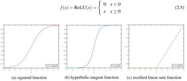
2.2.2 Activation Functions

It is desirable for an activation function, in the context of LSTMs, to produce an output that is both bounded and limited for all cases. This means that the function must have a predictable behaviour, and will not output values with large magnitudes independently of the input. Furthermore, it is desirable that the chosen function is fully differentiable. Some possibilities for activation functions follow below.

The Heaviside step function performs as a simple, binary-valued function with a threshold, and a discontinuity at x = 0 (Equation 2.2).

f(x) =H (x) (

0 x< 0

1 x≥ 0 (2.2)

The sigmoid function,Figure 2.2a, allows for a more complex behaviour, as it is a real-valued function, with its output moving slowly in the interval [0, 1] (Equation 2.3).

f(x) = σ (x) = 1

6 Problem Characterisation

The hyperbolic tangent function,Figure 2.2b, is very similar to the sigmoid, with its output moving slowly in the interval [−1, 1] (Equation 2.4).

f(x) = tanh(x) =e x_{− e}−x

ex_{+ e}−x (2.4)

The rectified linear unit function,Figure 2.2c, introduces a non-linearity at x = 0, which can be used for decision making (Equation 2.5).

f(x) = ReLU(x) = ( 0 x< 0 x x≥ 0 (2.5) -5 -4 -3 -2 -1 0 1 2 3 4 5 x 0 0.1 0.2 0.3 0.4 0.5 0.6 0.7 0.8 0.9 1 y sigmoid

(a) sigmoid function

-5 -4 -3 -2 -1 0 1 2 3 4 5 x -1 -0.8 -0.6 -0.4 -0.2 0 0.2 0.4 0.6 0.8 1 y tanh

(b) hyperbolic tangent function

-5 -4 -3 -2 -1 0 1 2 3 4 5 x 0 0.5 1 1.5 2 2.5 3 3.5 4 4.5 5 y ReLU

(c) rectified linear unit function

Figure 2.2: Examples of activation functions

Concerning the criteria introduced for choosing an activation function, it is concluded that both the sigmoid and the hyperbolic tangent are good candidates for activation functions. This is supported by current work in the literature on LSTMs, which often uses both the sigmoid and the hyperbolic tangent functions. As for the Heaviside function, it is not differentiable, thus it was not chosen. The rectified linear unit function, despite being widely used in other ANNs, has little used in LSTMs, as its output is neither bounded nor differentiable [4].

2.2.3 Forming ANNs

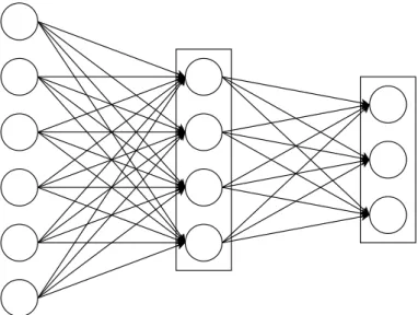
As mentioned earlier, the perceptron can be used as a basic building block to form increasingly complex models, resulting in an ANN, as depicted inFigure 2.3. The main advantage of doing this is the ability of mixing results from different inputs, thus obtaining a model that performs complex computations while using simple linear operations.

Specifically, this is performed by chaining perceptrons to one another, usually in a directed acyclic graph. The perceptrons are organised in groups of nodes occupying identical hierarchical positions called layers, in which the output from each neuron is used as an input to all the neurons in the following layer.

Neurons in ANN implementations are usually organised into the following layers: • Input layer: accepts all the inputs and performs the first round of computations;

2.2 Artificial Neural Networks 7

Figure 2.3: An ANN with three connected layers. Its input layer accepts 6 inputs, its hidden layer contains 4 perceptrons, and its output layer generates 3 different values.

• Hidden layers: perform intermediate computations; there is no restriction to the number of hidden layers, nor to the number of perceptrons in each layer;

• Output layer: performs final computations and outputs an intelligible value.

Each layer, similarly to a perceptron, contains its set of weights, which are used during infer-ence mode to predict an output based in the input pairs given to it.

2.2.4 Training

As mentioned insubsection 2.2.1, the ANN needs to be trained before being able to accurately perform inference. In line with the scope of this work, the training procedure explained below focuses on a supervised learning algorithm using labelled samples.

During training, all the elements of the training set are traversed, and each of these passes is called a training epoch. The duration of each epoch varies depending on the input length of the training set and on the type of network.

Before any training epoch occurs, the network weights are initialised, preferably to a set of small random values. Afterwards, each training epoch is composed by a two-step process. First, forward propagation is performed, and then backward propagation occurs.

Forward propagation begins by computing all the activation values of the network. The activa-tion values for the output layer are then compared against the existing labels using a cost funcactiva-tion for measuring the accuracy of the network. A common choice is the mean-squares error function inEquation 2.6, which averages the error for all m training samples and for each K output class, with (hW(x(i)))krepresenting the predicted value for each sample.

J(W ) = −1 m m

∑

∑

y(i)_k log((hW(x(i)))k) + (1 − y (i)

k ) log(1 − (hW(x(i)))k) i

8 Problem Characterisation

Backward propagation then uses these values to minimise the cost function by optimising the weight parameters. At this stage, the gradients, which give the direction of maximum change of the cost function for each weight, are computed for each node, and determine the influence of each weight in the total error. The weights are then adjusted from outputs to inputs, and the magnitude of this adjustment tuned by changing the learning rate. The learning rate consists of a tuning parameter that determines the step size in each iteration, with the goal of moving towards a minimum of the cost function. The choice of this parameter is relevant since, if it is too large, the function may never converge, whereas if it is too small, convergence might take many iterations and needlessly increase computation times.

A commonly used algorithm for backward propagation is the gradient descent. This algorithm, which is exemplified inAlgorithm 1, updates the weights iteratively after starting from a random position. Backward propagation can be performed over each sample separately, or in a batch of samples (that is, a number of samples bundled together), which can simplify computations.

2.3

Recurrent Neural Networks

2.3.1 Overview

A Recurrent Neural Network (RNN) can be seen as a directed cyclic graph, meaning that the output from one RNN cell is given as an input to another cell (that is essentially a copy of itself), as depicted in Figure 2.4, This structure, which is suitable to manipulate sequences and lists, enables RNNs to deal with information that contains a sequence (i.e. that depends of previous inputs), such as speech recognition or natural language processing.

x y x1 y₁ x2 y₂ x3 y₃ xt y_t

=

...

Figure 2.4: An RNN and its unrolled equivalent [5]

RNNs can be trained using a number of algorithms, backward propagation through time being a common solution. This is similar to backward propagation insubsection 2.2.4, but now taking into account the unrolling of the network through time.

The output data obtained at time t, yt, is mainly influenced by data obtained immediately prior to it, as earlier values cannot exert much influence. This happens because of the difficulty, during training, for the error at yt to backpropagate to the initial values of the sequence. This represents the vanishing gradients problem, which also occurs with ANNs. Specifically, in the context of

2.3 Recurrent Neural Networks 9

RNNs, this problem results in an increasing difficulty of an RNN to relate long dependencies between present and past information.

Algorithm 1 Backward propagation using gradient descent for the network inFigure 2.3 Training set: {x(i)_{, y}(i)_}

Activation value: a(l)_j Output value: z(l)_j Weight matrix value: W_j(l)

Gradient: δ_i(l)

Gradient accumulator: ∆(l)_{i j}

Learning rate: λ

for all pair i, node j, layer l do ∆(l)_{i j} ← 0

end for

for all i of m in training set do

function FORWARDPROPAGATION

for all j nodes in layer do . Computed from input to output a(1)_j ← x(i)_j z(2)_j ← W_j(1)a(1)_j a(2)_j ← hW(z(2)_j ) (add a(2)₀ ) z(3)_j ← W_j(2)a(2)_j a(3)_j ← hW(z(3)j ) end for end function

function BACKWARDPROPAGATION

for all j nodes in layer do . Computed from output to input δ_i(3)← a(3)_j − y(i)_j ∆(2)_{i j} ← ∆(2)_{i j} + δ_i(3)(a(2)_j )T δ_i(2)← (W_j(2))Tδ_j(3)◦ (a(2)_j ◦ (1 − a(2)_j )) ∆(1)_{i j} ← ∆(1)_{i j} + δ_i(2)(a(1)_j )T end for end function end for

for all l layers do

D(l)_{i j} ←_m1(∆(l)_{i j} + λW_{i j}(l)), j 6= 0 D(l)_{i j} ← 1 m(∆ (l) i j ), j = 0 end for

10 Problem Characterisation

2.3.2 Long Short-Term Memory Networks

Long Short-Term Memory Networks (LSTMs) are a variation of RNNs that use a memory con-troller to be able to retain long-term dependencies [6].

The architecture of an LSTM cell is depicted inFigure 2.5. The core idea behind these net-works is the cell state Ct, which serves as a memory element [5]. This state is controlled by four network gates that have the ability to let information through:

• Forget gate, ft: decides whether to keep or discard information in the cell state Ct−1, thereby controlling the cell state;

• Input gate, it: decides which values to be updated;

• Update gate, zt: decides the candidate values (i.e. the flow of information) to be added to the cell state Ct;

• Output gate, ot: decides which values (i.e. the flow of information) to output to ht.

C_t-1 × ＋ ft σ ot σ it σ zt tanh × h_t × h_t Ct h_t-1 x_t tanh

Figure 2.5: An LSTM cell [5]. Rectangles show neural network layers and their corresponding activation functions, and circles denote a pointwise () operation. Arrays are represented by lines, with array concatenation and copying shown by line merging and forking, respectively.

The hidden state ht serves as the output of the cell. It can be passed through a softmax fil-ter, which returns the output probabilities. By retrieving the index of the maximum probability value out of the softmax layer (or by simply returning the maximum value of ht), it is possible to determine the predicted value.

The update gate zt also shields the LSTM from the vanishing gradients problem. Because the cell state Ct can acquire values very close to 0 or 1, the existing information in it is able to persist in the system for many iterations.

2.4 High Level Synthesis 11

There is a number of possibilities to formulate the equations for inference with an LSTM. In Equation 2.7, a solution that maximises parallel computations at time t is shown.

ft = σ ([Wi fxt+ bi f] + [Wh fht−1+ bh f]) it = σ ([Wiixt+ bii] + [Whiht−1+ bhi]) zt = tanh([Wizxt+ biz] + [Whzht−1+ bhz]) ot = σ ([Wioxt+ bio] + [Whoht−1+ bho]) ct = ft ct−1+ it zt ht = ot tanh(ct) (2.7)

All weights and biases are highlighted in bold. Defining N as the input dimension, M as the output dimension, and H as the dimension of the hidden layer, its description follows:

• Wimatrices represent weights associated to the input pairs xt, and contain H × N elements

• Whmatrices represent weights associated to the hidden state ht−1, and contain H × H ele-ments

• bivectors represent bias values associated to the input pairs xt, and contain H elements

• bhvectors represent bias values associated to the hidden state ht−1, and contain H elements

The usage of the hidden state can vary depending on the requirements of the network. It is possible to randomly generate a hidden and cell state vector for every input pair prediction, which constitutes a stateless network. Another option consists of using the hidden and cell state vectors to compute the new predicted values, which constitutes a stateful network.

A number of modifications have been suggested throughout the years. Namely, the introduc-tion of a forget gate [7] and peepholes have been suggested. Upon considering their usefulness, the former will be used in this work, whereas the latter will be discarded, as it has been proved to have a minimal impact on performance [8] while requiring greater resources.

2.4

High Level Synthesis

2.4.1 Overview

Traditionally, programming on FPGAs requires the use of a Hardware Description Language (HDL) such as Verilog or VHDL, which is then translated to Register Transfer Level (RTL) that specifies the design using parallel processes that operate on vectors of binary or simple data type signals. With the rapid increase of complexity in System-on-a-Chip (SoC) designs, the need arose for using design abstractions that were faster and more effective to implement than RTL.

This motivated the development of High Level Synthesis (HLS) tools that could use a higher-level programming language (such as C/C++) to specify a synthesisable RTL implementation [9]

12 Problem Characterisation

for ASICs and FPGAs while hiding several implementation details. A HLS tool thus provides a programming development environment more similar to that of standard processors.

In recent years, Xilinx developed a tool for this purpose, named Vivado HLS. This tool accepts C, C++ or SystemC (which is a subset of C++), however C++ code interpretation is optimised. The code is then translated to HDL and described at RTL level. The source code can be compiled and verified using tools written for C/C++ for interpreting, analysing, and optimising the code.

When it comes to writing C/C++ code, Vivado HLS tools are similar to those of processor compilers for interpretation, analysis and optimisation of programmes, while targeting FPGA sys-tems. Because of this, application code for Vivado HLS is similar to standard C/C++ code (with the exception of dynamic memory allocation, which is not supported because of the memory ar-chitecture of the FPGAs), so it can normally analyse operations, conditional statements, loops, and functions [10]. Variables, classes and structs can be assigned to registers, whereas arrays are mapped to BRAM structures. Besides this, code in C/C++ can be synthesised without explicitly declaring any clock signal. These characteristics abstract the programmer from several low-level details and make HLS easier to use in comparison with HDL tools.

Despite this, programming in Vivado HLS is a more challenging task than C/C++ program-ming for software, while providing less control over the generated hardware than traditional HDL implementations. Although a large subset of C/C++ code that is not optimised for hardware is often synthesisable and functional, it usually results in slow, cumbersome RTL code, due to the in-herent differences between general-processing and parallel programming. Thus, in order to obtain efficient, synthesisable code, the programmer needs to take into account the hardware structure of the FPGA and programme accordingly. In some instances, optimisations are highly dependent on the coding style, as the HDL output can only be optimised (or at all used) by Vivado HLS if it obeys to some canonical form described by Xilinx. Besides this, there are a number of code op-timisations that can only be performed by programmer-defined pragmas. Pragmas are directives used by Vivado HLS to perform local code optimisations. These are instantiated in the code or by a directives script. This means that, in order to obtain good results under HLS, the programmer needs to have a grasp not only of the underlying hardware, but also of the specific structures and optimisations that can be performed by the HLS software that is being used.

2.4.2 Pragmas

With the goal of directing further performance and area optimisations, Vivado included a set of optimisation directives, called pragmas [9]. The relevant options to be used or related with this work are explained below.

Array Partitioning

#pragma HLS ARRAY_PARTITION variable=<name> type <factor=N> dim=<N>1and

1_{factorspecifies in how many blocks the array is split into; dim specifies the dimension in which the transformation} is performed, thereby allowing the programmer to optimise the access of the array for a specific dimension.

2.4 High Level Synthesis 13

#pragma HLS ARRAY_RESHAPE variable=<name> type <factor=N> dim=<N>

These directives can modify the arrangement of arrays mapped into memory. Vivado HLS defaults array implementation to BRAM, which has a maximum of two data ports. This often constitutes a bottleneck by limiting the number of read and write instructions possible per clock cycle. With these directives, Vivado provides three types of array partitioning, as depicted in Figure 2.6:

• Block: division into equally sized blocks of consecutive elements of the original array • Cyclic: division into equally sized blocks by interleaving the elements of the original array • Complete: fully splits the array into its individual elements by placing them in individual

registers 0 1 2 … N-3 N-2 N-1 cyclic block complete 0 1 … (N/2-1) N/2 … N-2 N-1 0 2 … N-2 1 … N-3 N-1 0 1 … N-2 N-1 2

(a) array partitioning

0 1 2 … N-3 N-2 N-1 cyclic block complete N/2 … N-2 N-1 0 1 … (N/2-1) … 1 N-1 0 LSB MSB 1 … N-3 N-1 0 2 … N-2 LSB MSB array[N] array[N/2] array[N/2] array[1] MSB LSB (b) array reshaping

Figure 2.6: Array transformations provided by Vivado HLS [9]

ARRAY_PARTITION and ARRAY_RESHAPE differ solely on the method used for this parti-tioning. Whereas the former opts for physically splitting the arrays into multiple physical arrays in order to obtain more read/write ports, the latter allows parallel access of data via vertical map-pingof the words, which bundles several elements of the array into a single element with a larger bit-width.

Interfaces

#pragma HLS INTERFACE mode port=<name> <bundle=string> register <register_mode> <depth=N> <offset>

It provides the ability to specify how the RTL ports from the function description are created. By default, Vivado HLS defaults mode to ap_ctrl_hs, which is used for block-level I/O and implements a handshake protocol (i.e. it indicates when to start design operation, and when the design is idle, done, and ready for new input data). On the top-level, it also supports AXI interface modes [11]:

• AXI4-Stream (axis): defines a single channel for transmission of streaming data that can be used to burst an unlimited amount of data, and is ideal for transferring streams of data (e.g. audio, video file);

14 Problem Characterisation

• AXI4-Lite (s_axilite): similar to AXI4-Master (but without burst support), it can be used to transfer small amounts of data (e.g. a parameter in a variable);

• AXI4-Master (m_axi): used for transferring small amounts of data, and preferred for trans-ferring bursts of data with high transfer speeds (e.g. a parcel of a wide array of data). The usage ofm_axirequires specifying the depth of the FIFO used in simulation, which corre-sponds to the amount of data accesses to the array, otherwise RTL Co-Simulation will not work properly.

Using the AXI4 protocol can simplify the connection of an IP block with other elements in the architecture due to its wide support. Moreover, Vivado HLS automatically generates device drivers for managing IP blocks with AXI4-Lite ports. By using the offset option, this can be used to specify the starting pointer of an array, which can then be used by the accelerator to access DDR memory according to its needs.

Data and Control Flow

#pragma HLS LOOP_FLATTEN <off>

It enables nested loops to be collapsed into a single loop with improved latency, thereby saving clock cycles (entering and exiting a loop in RTL requires 1 clock cycle). It can only be used with loops where only the innermost loop has body content, and where all loop bounds are constants (however, the outermost loop can be a variable).

#pragma HLS UNROLL <factor=N> <region> <skip_exit_check>

It enables loop unrolling, either completely or partially by a factor of N. This enables all loops to execute in parallel, however this is only possible if no data dependencies exist between different iterations.

#pragma HLS PIPELINE <II=N> <enable_flush> <rewind>

It enables function and loop pipelining, however, only loop pipelining will be described due to the scope of this work. It tries to implement a design with an Initiation Interval (II), which consists of the number of clock cycles between the start times of consecutive loop iterations, specified by the programmer. It defaults to 1, and if the value cannot be achieved, Vivado HLS tries to imple-ment a design with the minimum II possible. Loop pipelining allows the operations in the loop to overlap, thus leading to significant reductions in the number of clock cycles during sequential operation. The scenario depicted in Figure 2.7 illustrates the results achieved with pipelining: whereas the sequential version has an II of 3, and requires 8 cycles until the last output is written, the pipelined version has an II of 1, and requires only 4 cycles to write the last output. One caveat of this directive is that, despite only pipelining the specified region, it forces loop unrolling over all nested loops below the pipeline. Furthermore, using pipelines in Vivado HLS requires the use of constants for all loop bounds.

2.4 High Level Synthesis 15 void func(m, n, o) { for (i = 2; i >= 0; i--) { op_Read; op_Compute; op_Write; } } 3 cycles 1 cycle RD CMP WR RD CMP WR RD CMP WR RD CMP WR RD CMP WR RD CMP WR 8 cycles

Without Loop Pipelining With Loop Pipelining

4 cycles

Figure 2.7: Loop pipelining with Vivado HLS [9]

#pragma HLS INLINE <option>

It removes a function as a separate entity in the hierarchy and inserts (i.e. inlines) it in whatever code block it is called, which in some cases enables operations within the function to be shared and optimised more effectively (e.g. by reducing function call overhead). This is often performed automatically for small functions by Vivado HLS. An off option is provided, which is convenient for large functions. With it, block interfaces are clearly defined, which allows for an easier tracking of data dependencies, thereby enabling greater block-level parallelism.

2.4.3 Data Types

Vivado HLS provides a number of libraries to help during design implementation. Namely, it provides a set of libraries that enable the creation of customised datatypes.

The most important of these isap_fixed.h. It enables the definition of fixed-point data types according to the needs of the design, using the form ap_[u]fixed<W,I,Q,O,N>. The explanation for each parameter, as per [9], follows below.

• W: number of bits for the word length • I: number of bits for the integer part

• Q: quantisation mode for when greater precision is generated than can be defined by the decimal component of the variable

• O: overflow mode for when a value that exceeds the possible representation is achieved • N: number of saturation bits in overflow wrap modes

A library for integers,ap_int.h, is also defined. It allows the definition of signed and un-signed integers with variable bit length, using the form ap_[u]int<W>, with W defining the num-ber of bits of the word length.

16 Problem Characterisation

2.5

Summary

In this chapter, a number of key concepts concerning the present work have been discussed. The brief introduction to Machine Learning inSection 2.1allowed to understand the motivation behind its widespread usage, not least its ability to learn and solve problems without explicit program-ming. Afterwards, the explanation on ANNs inSection 2.2, and afterwards of RNNs and LSTMs inSection 2.3, enabled the comprehension of their utility in different scenarios (namely, the ade-quacy of ANNs for a number of problems, and the capability of RNNs, and concretely LSTMs, to overcome the issues of ANNs when dealing with time dependencies). InSection 2.4, the concept of High Level Synthesis, which has the potential of significantly simplifying hardware synthesis by using a high-level language for creating RTL descriptions, was introduced.

Chapter 3

State of the Art

This section provides an overview of the state of the art for LSTM networks.Section 3.1provides an overview of the potential of LSTMs, and shows some examples of work performed with this type of networks. Section 3.2describes some notable, state-of-the-art LSTM implementations on FPGA.Section 3.3provides a summary on the topic.

3.1

LSTM Applications: Overview

LSTM networks are currently, due to their superior performance, a state-of-the-art algorithm for a wide range of applications, namely for prediction and time-series classification of data. Therefore, significant work has been performed with this type of RNN.

To illustrate, some examples in the academia include a prize-winner handwriting algorithm specialised in unsegmented cursive writing [12], a speech recognition algorithm focused on key-word spotting [13], and a music composition algorithm using a text-based network [14]. The application of LSTM networks is also common in the industry, examples of this being a probabil-ity forecasting algorithm produced by Amazon [15], and a keyboard gesture decoding algorithm developed by Google [16].

The wide adoption of LSTM solutions, and their varying performance and resource require-ments, led to their implementation in several hardware platforms.

A number of frameworks is available for use with CPUs and GPUs, such as Keras1, PyTorch2, and TensorFlow3. These implementations are usually optimised for high performance by using Single Instruction, Multiple Data (SIMD) and multi-threaded instructions on CPUs, and CUDA or OpenCL kernels on GPUs.

1_{https://keras.io} 2_{https://pytorch.org} 3_{https://tensorflow.org}

18 State of the Art

Hardware-level solutions have also been implemented, with ASICs being used for specialised applications with a fixed network topology. Furthermore, a number of solutions on FPGA have been explored.

3.2

LSTM Implementations on FPGA

Over the last few years, a number of LSTM implementations on FPGA have been developed. Some proposals focus on optimising the LSTM network to be used by applying pruning and quan-tisation techniques. Briefly, the former technique consists of setting some weights of the LSTM to zero, so that they can be discarded during computations. Generally, the resulting pruned weight matrices are sparse, which is problematic for hardware as it requires non-optimal, random data accesses. Other proposals put a greater emphasis on optimisations performed at the architectural level, namely by increasing computation parallelism. With this in mind, some relevant FPGA im-plementations are described below.

Fonseca et al. [17] developed one of the first FPGA implementations of an LSTM. It stores the LSTM network and input pairs in on-chip memory for faster access, and uses a 18-bit fixed-point system for data representation, chosen to make full usage of the DSP slices on the FPGA. A network with a maximum hidden dimension of 256, for an input dimension of 2, was achieved on a Xilinx Zynq XC7Z045 SoC. The implementation was tested with an 8-bit adder.

Wang et al. [18] introduced a pruning solution to tackle the uneven memory accesses that arise from unstructured pruning. Moreover, a framework for implementing various LSTM variations on FPGA, C-LSTM, is presented.

The authors propose to compress the LSTM model by using block-circulant matrices, where each row vector is the circulant transformation of the row vectors. By dividing the original matrix into blocks, it is possible to greatly compress the matrix by reducing the number of parameters. However, this comes at the cost of accuracy, specially because there is no prior selection of the weights to be pruned, which might be important for the network to operate appropriately. Using circulant matrices enables the use of a Fast-Fourier Transform, thus reducing the complexity of the computations. It is important to note that this requires pre-processing the data, which will add up to the overall system latency. A double-buffering mechanism is used to improve the parallelism of computation in the system.

The C-LSTM framework presented, in turn, consists of two distinct parts, one concerning system training on TensorFlow, and another focused on implementation in FPGA that uses a scheduling graph and a code generator to produce synthesisable code, constituting a structured-compression technique.

The solution is tested on the TIMIT [19] dataset, where the authors claim to use weight ma-trices up to 14.6x smaller and 3.7x less computationally-intensive in comparison with the original

3.2 LSTM Implementations on FPGA 19

matrices, while incurring in a performance degradation in comparison with an uncompressed ma-trix of up to 1.23%.

Cao et al. [20] proposed a pruning solution with bank-balanced sparsity. In this paper, the method split each matrix row in multiple equally-sized subrows, applying weight pruning inde-pendently and obtaining the same number of non-zero values. With this, the authors use a more structured sparsity pattern, and obtain better results on hardware, and load balancing between BRAMs is achieved. The input pairs are stored in an array buffer, and partitioned in blocks to enable parallel access. This is possible thanks to the bank-balanced architecture used, which guar-antees that every array has the same number of elements, and that at most one element from each block is accessed every clock cycle. Additionally, double-buffers are used to overlap data transfer and computation operations.

The authors claim that this bank-balanced sparsity method obtains higher model accuracy than block sparsity by preserving the unstructured distribution of non-zero weights for each bank, while at the same time achieving similar performance in comparison with unstructured block sparsity.

The bank-balanced sparsity solution, with a 16-bit fixed-point representation, is compared against a 32-bit floating-point representation baseline. For PTB [21] and TIMIT, prediction accu-racy is maintained for up to 80% and 90% sparsity, respectively.

Wang et al. [22] dealt with network compression techniques, which make use of an algorithm previously developed by the authors, HOCA [23], and perform memory access pattern optimisa-tions.

The HOCA algorithm consists of two steps: initialisation and training with clipped gating and quantisation, and top-k pruning. First, a technique called clipped gating is used, which sets the activation function to 0 if its value falls below a pre-determined threshold. For quantisation, a fixed-point quantisation scheme is introduced, which uses a rounding mechanism to the nearest decimal place achievable in fixed-point, and a logarithmic scheme that quantises each weight to the nearest power of two. The algorithm finishes by performing top-k pruning, which generates structured sparse matrices by concatenating all weight matrices, grouping them in sets, and then pruning until at most k non-zero elements remain in each group. The aforementioned procedures are performed on software.

A number of architectural improvements are also performed. Double-buffers are used to over-lap data transfer and computation operations. Computation of the input pair and hidden state com-ponents for each gate is performed sequentially. During computation, weight values are fetched from a row at a time. While this promotes input pair value re-utilisation, as these values only need to be cached once, it results in little weight reuse, as this requires the batch size chosen to be small and dependent on the input dimension. The network is architected so that an arbitrary number of LSTM layers can be loaded.

The solution is tested on the TIMIT dataset, where the authors claim to use weight matrices up to 32x smaller and with a computation complexity up to 22.61x lower in comparison with the

20 State of the Art

original matrices, without incurring any performance degradation.

Rybalkin et al. [24] released an open-source library extension for HLS which implements a parallelisable architecture of LSTM layers on FPGA. With this library, the authors claim to enable parametrised performance scaling that offers different levels of parallelism. It uses on-chip memory with a variable-width fixed-point system. The architecture is based on a previous solution produced by the authors [25].

An LSTM with two layers is used. This approach results in increased computation parallelism, as a forward layer (i.e. reads input pairs from left to right) and a backward layer (i.e. reads input pairs from right to left) perform computations in parallel. The layers are concatenated at their outputs. Memory access patterns are rearranged to make use of this architecture. Afterwards, further processing is performed using a linear layer, whose output is passed to a max layer that determines the maximum (i.e. predicted) value. Its parametrisable architecture allows, on the one hand, to provide concurrent execution of multiple LSTM cells and, on the other hand, to divide the execution of a single LSTM cell over multiple cycles.

The HLS library extension enables usage of a fixed-point, variable-width data type for the weight matrices, input and output activations, and recurrent activations4. The bit-width of the input pairs is not described, although it is set at 5 bits in [25].

The solution is tested on a custom OCR dataset, with a reported test accuracy above 90% for any combination of bit width between 1-8 bits for each data type, and a throughput increase of up to 5.7x when comparing a 1-bit (i.e. binarised) to an 8-bit implementation.

Que et al. [26] presented an implementation in which the operations of the LSTM are reor-ganised to eliminate data dependencies. Additionally, a block-batching solution is used, which fetches partial square blocks for each weight matrix and for a batch of input pairs. A double-buffering mechanism is used to improve the parallelism of computation in the system. The system uses a 16-bit fixed-point system for data representation.

To optimise the operations, a technique is used that first performs partial computations over the input pair values, (with its data re-usage dependent on the chosen block size) without using the corresponding hidden states. The purpose of this is to allow the next inference to occur without stalling the system pipeline. In this solution, the weight matrices are not split into their input pair and hidden state components. The weight matrices are partially cached along the columns, and fully cached along the rows. The values output by the system are obtained directly from the LSTM (i.e. no fully connected layer is used).

The proposed block-batching technique, for computational purposes, combines the input pair and hidden state weight matrices (for each gate) into a single matrix, resulting in the sequential computation of each of these components. To do this, the input pair values and the previous hidden state are concatenated into a single input array. The blocking mechanism consists of splitting the weight matrices in column blocks, and then fully fetch them along the rows. In turn, the

3.3 Summary 21

concatenated input array is likewise partially fetched, and the computations for each component are performed. The batching mechanism consists of fetching several concatenated input arrays in a single memory access. The goal is to have a computation time equal or greater to the transfer time, so that memory caching is transparent (i.e. it does not impact system performance).

The solution is tested with output data from the average pooling layer of the Inception-v3 network, which was pre-trained in the ImageNet dataset. When compared with CPU and GPU solutions making use of TensorFlow5, it is reported to provide speed-ups of up to 23.7x and 1.3x respectively, with a corresponding 208x and 19.2x reduction on power consumption. A compari-son between the accuracy achieved in each of these platforms is not explicitly stated.

3.3

Summary

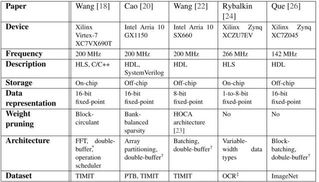
A summary of the characteristics of each solution is presented inTable 3.1. Paper Wang [18] Cao [20] Wang [22] Rybalkin

[24] Que [26] Device Xilinx Virtex-7 XC7VX690T Intel Arria 10 GX1150 Intel Arria 10 SX660 Xilinx Zynq XCZU7EV Xilinx Zynq XC7Z045 Frequency 200 MHz 200 MHz 200 MHz 266 MHz 142 MHz Description HLS, C/C++ HDL, SystemVerilog HDL HLS HDL

Storage On-chip Off-chip Off-chip On-chip Off-chip

Data representation 16-bit fixed-point 16-bit fixed-point 8-bit fixed-point 1-to-8-bit fixed-point 16-bit fixed-point Weight pruning Block-circulant Bank-balanced sparsity HOCA architecture [23] No No Architecture FFT, double-buffer*, operation scheduler Array partitioning, double-buffer† Batching, double-buffer† Variable-width data types Block-batching, dobule-buffer†

Dataset TIMIT PTB, TIMIT TIMIT OCR‡ ImageNet

* _{Used to improve computation parallelism}

† _{Used as a ping-pong buffer, i.e. for simultaneous computations and data transfer}

‡ _{Custom dataset}

Table 3.1: Summary of the described LSTM implementations on FPGA

In conclusion, when implementing LSTM networks on FPGA, memory storage of the weights and the input pairs is one of the limiting factors for the achieved performance. To overcome this, some proposals opt for pre-processing the weight values, by performing pruning or quantisation to reduce the size of the input pairs and weight matrices in memory. As for the storage itself, some papers opt to store the values on-chip, while others opt to store all values off-chip, and

22 State of the Art

then transferring them to the memory in the fabric on-the-go. In several instances, double-buffer techniques are used to overlap data transfer with computation operations to avoid large latencies.

Regarding weight pruning, it is a commonly-used technique both for FPGAs and for other platforms to achieve good predictions with less memory and fewer computations. Additionally, these techniques may be used on top of other architectural optimisations. Nevertheless, it com-monly happens that pruning techniques do not take into consideration the influence of each weight in the final result, which may lead to removal of important values, and as a result to performance degradation of the network. Thus, pruning should be tailored depending on the network to be im-plemented. Besides this, it is necessary to consider the implications of using pruning on hardware due to its greater implementation complexity. For instance, in many cases weight pruning leads to random memory accesses, which are slower, and may require additional memory to store the positions corresponding to the valid weights after pruning. Because the scope of this work focuses on a general LSTM implementation, pruning techniques will not be considered.

With respect to architectural improvements, many solutions use double-buffer techniques to speed up network performance. Because of their usefulness, double-buffers will be used through-out this work.

Batching (i.e. forming a bundle of input pairs) is also commonly used, because it enables greater weight reuse, thus leading to fewer accesses to memory. Nevertheless, most techniques can only use batching to a limited extent, because weight matrices are usually fully fetched alongside one of its dimensions. This approach has two issues. First, it uses a significant amount of memory, which immediately limits the number of input pair values that can be batched to memory. Second, fully fetching a matrix in any of its dimensions requires keeping more temporary accumulators used for storing the results of the matrix-vector multiplications between the weight matrices and the input pairs without increasing system parallelism.

As for data representation, the fixed-point proposals mentioned in this chapter do not specify the position of decimal place, or the behaviour of the network when overflow occurs. Changing any of these parameters might have severe implications on the accuracy of the network.

Another important aspect consists of the limitations of the networks that can be used in these accelerators. For the accelerators inTable 3.1that solely use on-chip storage, restrictions in terms of network size and input pair values will always be high because of the limited memory available inside an FPGA, even if reconfigurability is allowed. As for the off-chip variants, little is said about the scalability of the network except for Que et. al [26], who mention as further work the automatisation of the architecture to enable rapid development of new designs.

Additionally, most LSTM network implementations on FPGA only focus on inference. This happens for two reasons. First, the process of inference is composed mostly of matrix multipli-cations, which can be highly parallelised, and are ideal for implementing on an FPGA. Second, previous training implementations generally show poor performance. This happens because, when using fixed-point operators, the computed deltas contain small errors that accumulate during train-ing. While implementing a floating-point design could be a solution, it would, at the present moment, require a large amount of resources in the fabric.

Chapter 4

Proposed Architecture

This section describes the architecture of the accelerator proposed in this work.Section 4.1offers a high-level overview of the most relevant components of the system.Section 4.2introduces with more detail the building blocks of the accelerator, namely initialisation, buffering, computation, and auxiliary blocks.

4.1

Overview

4.1.1 Description

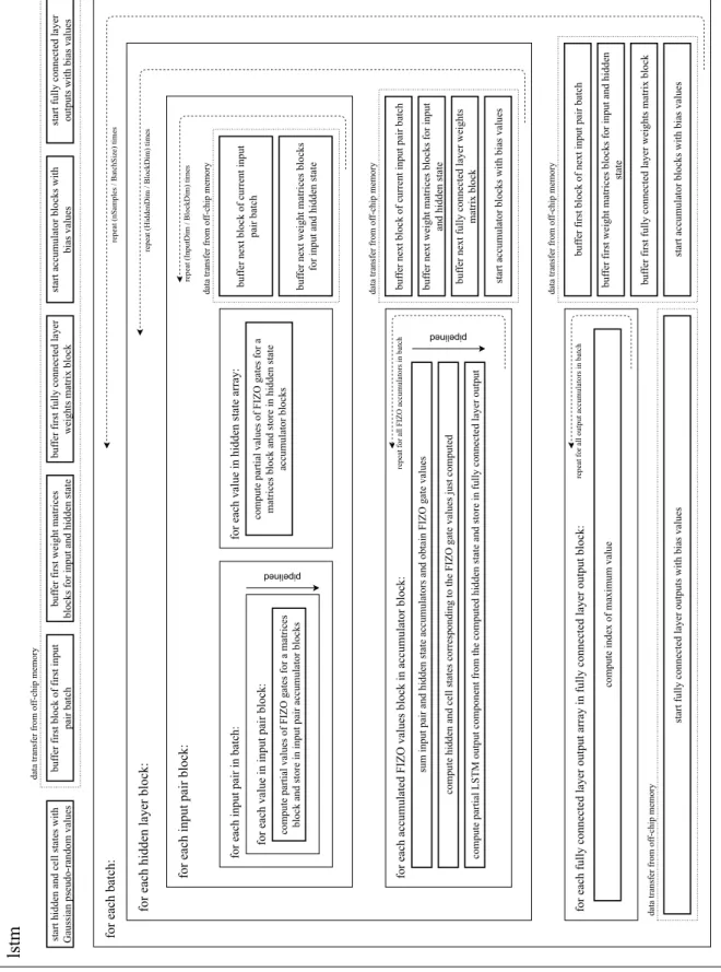
The proposed FPGA accelerator consists of a hardware implementation of a single LSTM cell, followed by a fully connected layer for dimensionality reduction.Figure 4.1depicts the complete architecture of the LSTM accelerator.

The accelerator was developed for usage with a network with arbitrary size. This means that using a set of input pairs with larger size than that available in on-chip memory is possible, since main memory storage is provided outside the reconfigurable fabric. To optimise data access, the accelerator performs buffering and computation operations in parallel. For this purpose, the accelerator uses a double-buffering technique that stores the input pairs and weight matrices of the current state on-chip, which enable fast access during computations, while simultaneously buffering the values from off-chip memory to be used in the next computation iteration.

The accelerator uses fixed-point arithmetic in its architecture. While still providing good re-sults, this approach results in less computational resources and provides lower latency on FPGAs. Additionally, the bit-width of the variables can be tuned for input pairs, weight matrices, hidden and cell states, and output values. This can be further used to reduce computational power (i.e. by using a maximum of 18 bits, only a single DSP is needed), and memory resources, with the potential of enabling faster manipulation of large networks.

24 Proposed Architecture

lstm

for each batch:

for each hidden layer block: for each fully connected layer output array in fully connected layer output block:

buf

fer next block of current input pair batch

buf

fer next weight matrices blocks for input

and hidden state

buf

fer next fully connected layer weights

matrix block

start accumulator blocks with bias values

for each accumulated FIZO values block in accumulator block:

for each input pair block:

for each input pair in batch:

repeat (InputDim / BlockDim) times

repeat (HiddenDim / BlockDim) times

repeat (nSamples / BatchSize) times

buf

fer first block of first input

pair batch

buf

fer first weight matrices

blocks for input and hidden state

buf

fer first fully connected layer weights matrix block

start accumulator blocks with

bias values

start fully connected layer outputs with bias values

start hidden and cell states with Gaussian pseudo-random values

data transfer from of

f-chip memory

for each value in input pair block: compute partial values of FIZO gates for a matrices

block and store in input pair accumulator blocks

for each value in hidden state array:

compute partial values of FIZO gates for a matrices block and store in hidden state

accumulator blocks

buf

fer next block of current input

pair batch

buf

fer next weight matrices blocks for input and hidden state

sum input pair and hidden state accumulators and obtain FIZO gate values

compute hidden and cell states corresponding to the FIZO gate values just computed

compute partial LSTM output component from the computed hidden state and store in fully connected layer output

repeat for all FIZO accumulators in batch

repeat for all output accumulators in batch

compute index of maximum value

buf

fer first block of next input pair batch

buf

fer first weight matrices blocks for input and hidden

state

buf

fer first fully connected layer weights matrix block

start accumulator blocks with bias values

start fully connected layer outputs with bias values

data transfer from of

f-chip memory

data transfer from of

f-chip memory

data transfer from of

f-chip memory

data transfer from of

f-chip memory

pipelined

pipelined

4.1 Overview 25

Consistent with the reconfigurable capability of FPGAs, this accelerator makes use of C++ templates to allow effortless specification of its main parameters, with an example presented in Listing 4.1.

The parameters can be divided into the following categories:

• Network dimensions: refers to the input, hidden, and output dimensions of the network. This allows effortless generation of different networks;

• Batch and block sizes: refers, respectively, to the number of input pairs to be simulta-neously processed by the accelerator, and the number of values from each input pair in a batch to be processed in one iteration. These parameters define the core functionality of the architecture, because they enable weight and input pair reuse;

• Data types: refers to the bit-width and integer-part width of input pairs, weight matrices, hidden and cell states, and output values.

// Defines network dimensions #define nSamples 500

#define InputDim 784

#define HiddenDim 128

#define OutputDim 10

// Defines batch and block sizes #define BatchSize 500

#define BlockSize 64

// Defines length for data types #define WidthInput 18 #define IntInput 2 #define WidthHidden 14 #define IntHidden 6 #define WidthMem 14 #define IntMem 6 #define WidthCalc 14 #define IntCalc 6 #define WidthOut 4

Listing 4.1: Architecture parameters with example values

4.1.2 Matrix computations

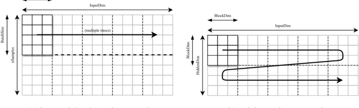
The core of the architecture consists of the strategy used to perform matrix computations. In an effort to perform data re-use when possible, a block-batching strategy with similarities to the one described in [26] was used.

26 Proposed Architecture

This block-batching technique consists of using a partial number of input pairs, which are bundled in a batch. With this, access to off-chip memory is optimised. In turn, each buffered input pair is only partially fetched from memory, and the partial array is multiplied by the partial forget, input, update, and output weight matrix blocks. These multiplications are performed along the row of both the input pair matrix, which contains all input pair values, and the weight matrices, as depicted inFigure 4.2. nSamples BatchSize InputDim BlockDim (multiple times)

(a) input pair batch matrix traversal

HiddenDim

BlockDim

InputDim BlockDim

(b) weight matrices traversal

Figure 4.2: Matrix traversal used in the block-batching technique

The computation results are stored in accumulators storing the temporary values for the input pair components of the forget, input, update, and output gates, which, after a full pass through the weight matrices rows, are used in the sigmoid and hyperbolic tangent functions to determine their value for each input pair. The computations are performed in a pipeline. Upon finishing the gate computations, the partial hidden and cell state arrays that were just computed for the input pair are ready to be used by the next input pair.

Unlike other solutions, the hidden state component is not computed for each input pair. In-stead, a single hidden state array is maintained, which is used by all input pairs to compute the hidden state component of the forget, input, update, and output gates. For this reason, this can be considered a batch-stateful network1, as it only stores the previous state of a whole batch. This enables the system to perform parallel computations for both the input pairs and the hidden state.

In order to save BRAM memory, only a single hidden and cell state array are maintained for the whole system. However, before being overwritten by the hidden and cell states of a new input pair, all hidden state values are used by the fully connected layer to compute their corresponding component on the output values, which are then, similarly to the computation results of the LSTM layer, stored in accumulators. Moreover, parallelisation is achieved, as each set of partial gate, hidden and cell state values of each input pair are computed in a pipeline.

It is also worth mentioning with more detail how the buffering and computation operations are performed at a higher level. First, both a batch of input pairs and a block of the weight matrices are traversed along their columns. Then, the next block of rows of the weight matrices is buffered, whereas the input pair batch is buffered again from the beginning. This means that the input