i
REMOTE ESTIMATION OF TARGET HEIGHT USING
UNMANNED AIR VEHICLES (UAVs)
Andrea Tonini
Dissertation presented as partial requirement for obtaining
the Master’s degree in Information Management
i REMOTE ESTIMATION OF TARGET HEIGHT USING UNMANNED AIR
VEHICLES (UAVs): Subtitle: Andrea Tonini
MEGI
2015 2015REMOTE ESTIMATION OF TARGET HEIGHT USING UNMANNED AIR VEHICLES (UAVs):
Andrea
ii
Instituto Superior de Estatística e Gestão de Informação
Universidade Nova de Lisboa
REMOTE ESTIMATION OF TARGET HEIGHT USING UNMANNED AIR
VEHICLES (UAVS):
by
Andrea Tonini
Dissertation presented as partial requirement for obtaining the Master’s degree in Information Management, with a specialization in Business Intelligence and Knowledge Management
Advisor: Prof. Marco Painho Co Advisor: Dr. Mauro Castelli
iii
SUBMISSION TO THE NTERNATIONAL PEER-REVIEWED OPEN
ACCESS JOURNAL ”SENSORS”
DEDICATION
Sensors 2019, 19, x; doi: FOR PEER REVIEW www.mdpi.com/journal/sensors
Article
1
REMOTE ESTIMATION OF TARGET HEIGHT
2
USING UNMANNED AIR VEHICLES (UAVs)
3
Andrea Tonini 1*, Marco Painho2 and Mauro Castelli2
4
1 European Maritime Safety Agency, Praça Europa 4, 1249-206, Lisbon, Portugal
5
2 NOVA IMS Information Management School, Campus de Campolide, 1070-312, Lisbon, Portugal
6
* Correspondence: [email protected]; Tel.: +351 961 059 638
7
Received: date; Accepted: date; Published: date (TBD)
8
Abstract: estimation of target height from videos is used for several applications, such as
9
monitoring agricultural plants growth or, within surveillance scenarios, supporting the
10
identification of persons of interest. Several studies have been conducted in this domain but, in
11
almost all the cases, only fixed cameras were considered. Nowadays, lightweight UAVs are often
12
employed for remote monitoring and surveillance activities due to their mobility capacity and
13
freedom for camera orientation. This paper focuses on how the height could be swiftly performed
14
with a gimballed camera installed into a UAV using a pinhole camera model after camera
15
calibration and image distortion compensation. The model is tailored for UAV applications
16
outdoor and generalized for any camera orientations defined by Euler angles. The procedure was
17
tested with real data collected with a regular-market lightweight quad-copter. The data collected
18
was also used to make an uncertainty analysis associated with the estimation. Finally, since the
19
height of a person who is not standing perfectly vertical can be derived by relationships between
20
body parts or human face features ratio, this paper proposes to retrieve the pixel spacing measured
21
along the vertical target, called here Vertical Sample Distance (VSD), to quickly measure vertical
22
sub-portions of the target.
23
Keywords: remote surveillance, target height, UAV, pinhole model, image distortion
24
compensation, Vertical Sample Distance (VSD)
25
26
1. Introduction
27
Unmanned Air Vehicles have been employed for more than two decades for military activities
28
[1] but, nowadays, they are also widely used for civil applications. In particular, non-coaxial
29
multi-rotors with weight below 4 kg [2] are often used to complement or, in some cases, even replace
30
fixed video cameras for monitoring and surveillance activities [3]. In fact, UAVs can bring a very
31
relevant added value compared with static installations: the possibility to transport and orient the
32
camera as needed, allowing to perform pre-established survey paths or even follow a specific target,
33
if needed [4].
34
Remote surveillance or monitoring activities may often require estimating the height of a target
35
via image analysis. The target could be a tree for example, in order to monitor its growing for
36
agricultural purposes [4], or a building, to follow contraction developments, or animals, to track
37
cattle growing [5]. However, as we may expect, remote height estimation from image analysis is
38
very often needed to define the exact stature of human beings. This is required to support the
39
identification of a person of interest [6], health care purposes [7] or even for marketing [8]. There is a
40
significant amount of studies in the literature dedicated to obtaining a person’s body height from a
41
video but, almost the totality of them considered data collected by static surveillance cameras. On
42
the other hand, UAVs have been mainly used for estimating features’ height for topographic or
43
urban mapping using Photogrammetry and LIDAR (Laser Imaging Detection and Ranging)
techniques (see for example [9], [10] and [11]). Photogrammetric techniques require having either a
45
double camera pointing at the same target or acquiring two images from different orientations of a
46
(static) feature. LIDAR data needs to be acquired by sophisticated devices installed in aircrafts
47
specifically designated for this kind of survey technique. In some studies [12], human height
48
estimation was performed with UAV using a machine learning approach. However, this approach
49
requires a quite intensive elaboration and it cannot be always performed in near real-time.
50
This paper focuses on how the height of a feature standing vertically from the ground can be
51
measured with a “regular” payload for lightweight UAVs, which is daylight Electro-Optical camera
52
installed into steerable gimbals. The goal is to estimate the height using a single image in a swift
53
fashion, possibly in near real-time, without the need for intense processing rapid situational
54
evaluation and quick decision making during the UAV flight. Moreover, we need to take into the
55
account that the UAV may operate outdoor, where topography and scene content may rapidly
56
change and the target may be a static feature, like a tree, or dynamic, like humans or animals.
57
A widely used approach for height estimation from video footages requires to identify, when
58
possible, vanishing lines in the scene (see for example [13], [14] and [15]). However, this approach
59
has relevant setbacks: defining vanishing lines may not be always possible in an image [16] and a
60
reference height in the scene is required to define the height of the target. Other authors have more
61
recently proposed to estimate the height of a person standing on a floor considering a pinhole
62
camera model after camera calibration and image distortion compensation [17]. A similar approach
63
was also used in [18] in combination with person body height estimation using interpupillary
64
distance, the comparison of these two methods showed that they are comparable and accurate.
65
It is here proposed an approach that foresees camera calibration and lens distortion correction
66
before calculating geometrically the height of the target using the pinhole camera model. This
67
procedure requires just a single image, or video frame, acquired with a camera fitted on-board of a
68
lightweight UAV. The correction for lens distortion allows generating an image as it was acquired by
69
a perfect pinhole system [19], which can be used for the mapping of a 3D scene to a 2D image.
70
However, the correction of an entire image may be very time-consuming. The approach here
71
described requires correcting just a very limited number of pixels, in order to reduce the elaboration
72
time for near real-time applications. On the other hand, the camera calibration [20] requires intrinsic
73
camera parameters, such as the focal length, and extrinsic parameters, such as camera position and
74
orientation. This paper analyzes how these parameters can be defined when dealing with UAVs, for
75
example the position of the camera is given by positional systems, like GPS.
76
The procedure was tested with real data collected with a regular-market lightweight quad-copter. A
77
measuring pole of known length standing vertically from the ground was used as a target for the
78
acquisition of several still images taken from different positions. For each shot, the height of the
79
target was calculated considering the procedure described above and compared with the real height
80
of the pole to assess the accuracy of the estimations. An analysis of the uncertainty was conducted to
81
analyze how the error associated with the camera-to-target distance can influence the accuracy of the
82
estimation.
83
The last part of this paper focuses on how estimating the vertical length of the target’s subparts,
84
which is particularly useful to define the exact human body height. In fact, the exact human stature
85
can be estimated in a video if the subject is standing vertically from the ground in a fully straight
86
pose. If the person has a different pose, such as standing relaxed with feet further apart and weight
87
on both feet standing relaxed with weight on one leg, we would manage to estimate just the height
88
of the body in that specific pose, see [6] and [21], not the real stature of the subject. In literature is
89
well known the relationship between the height of a person its body parts obtained via experimental
90
measures [22]. Therefore, the height a person who is not standing perfectly vertical can be derived
91
by relationships between body parts or and human face features ratio [23] face of the person is well
92
visible in the scene. It is here proposed to use the pixel spacing measured along the vertical target to
93
quickly estimate the length of body parts or face portions. The spacing in the vertical direction is
94
here called Vertical Sample Distance (VSD), which can be calculated as the GSD (Ground Sample
95
Distance, [24]) but perpendicular to the ground (vertical axis).
2. Methods
97
The first part of this section describes the basic principles of the pinhole model for computer
98
vision and processes for lens distortion compensation. After that, it is analyzed how computer vision
99
can be performed when dealing with cameras installed into UAVs. The last part of this section
100
presents and describe the method to estimate the height from still images or video frames acquired
101
with cameras installed into UAVs.
102
2.1. Pinhole camera model and computer vision
103
In computer vision, cameras are usually modelled with the pinhole camera model [28]. The
104
model is inspired by the simplest camera, where the light from an object enters through a small hole
105
(the pinhole). This model considers a central projection, using the optical center of the camera and an
106
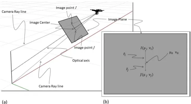
image plane (that is perpendicular to the camera’s optical axis, see Figure 1). In the physical camera,
107
a mirror image is formed behind the camera center but, often, the image plane is represented in front
108
of the camera center. The pinhole camera model represents every 3D world point P (expressed by
109
world coordinates xp,yp,zp) with by the intersection between the image plane and the camera ray
110
line that connects the optical center with the world point P (this intersection is called the image
111
point, noted with I in Figure 1).
112
113
114
Figure 1. Graphical representation a 3D world point P is projected onto a 2D Image Plane.
115
The pinhole camera projection can be described by the following linear model
116
117
[ μ𝑖 ν𝑖 1 ] = 𝐾[𝑅𝑇] [ 𝑋𝑝 𝑌𝑝 𝑍𝑝 1 ] (1)
118
Where K is the calibration matrix, defined as follow:
119
120
𝐾 = [ αμ γ μ0 0 αν ν0 0 0 1 ] (2)
121
αμ and αν represent the focal length expressed in pixels. μ0 and ν0 are the coordinates of the
122
image center expressed in pixels, with origin in the upper left corner (see Figure 1). γ is the skew
123
coefficient between the x and y axis, this latter parameter is very often 0.
124
The focal lengths, (which can be here considered as the distance between the image plane and
125
optical center) can be also expressed in terms of distance (e.g. mm instead of pixels) considering the
126
following expressions:127
128
𝐹𝑥= 𝑎μ 𝑊μ 𝑤μ (3) 𝐹𝑦 = 𝑎ν 𝑊ν 𝑤ν (4)129
Where 𝑤μ and 𝑤ν are, respectively, the image (or video frame) width and length, 𝑊μ is the
130
width and 𝑊ν the length of the camera sensor expressed in world units (e.g. mm). Usually, 𝐹μ and
131
𝐹ν have the same value, although they may differ due to several reasons such as flaws in the digital
132
camera sensor or when the lens compresses a widescreen scene into a standard-sized sensor. The
133
focal length 𝐹 (assumed here for simplicity that 𝐹 = 𝐹ν= 𝐹μ), 𝑊μand 𝑊ν can be also used to
134
calculate another important element, the Field of View (FOV) of the camera, which is the angular
135
extent of the observable world that is seen at any given moment and it may be different in μ and ν
136
directions (see Figure 2).
137
138
139
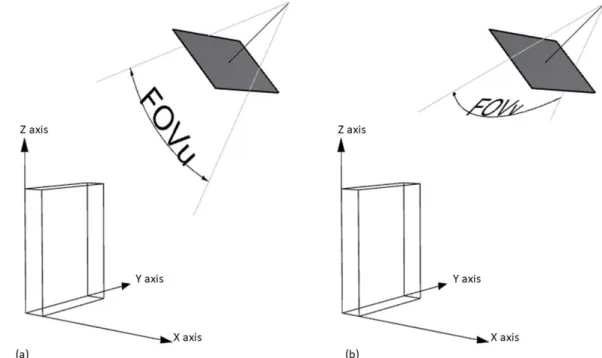
Figure 2 Graphical representation of the Field of View in the μ (a) and ν (b) directions
140
𝐹𝑂𝑉μ and 𝐹𝑂𝑉νcan be calculated as follow:
141
𝐹𝑂𝑉μ= 2 tan−1 𝑊μ
𝐹𝑂𝑉ν= 2 tan−1 𝑊ν
2𝐹 (6)
R and T in (1) are the respectively rotation and translation of the camera. These are the extrinsic
142
parameters which define the so called “camera pose”.
143
R is defined by the axis of rotation and the angle that describes the amount of rotation. In the
144
case of rotation around the X axis by an angle θx, the rotation matrix Rx is given by [19]:
145
146
𝑅𝑥= [ 1 0 0 0 cos(𝜃𝑥) −sin(𝜃𝑥) 0 sin(𝜃𝑥) cos(𝜃𝑥) ] (7)147
Rotations by θy and θz about the Y and Z axes can be written as:
148
149
𝑅𝑦= [ cos(𝜃𝑦) 0 sin(𝜃𝑦) 0 1 0 −sin(𝜃𝑦) 0 cos(𝜃𝑦) ] (8)150
𝑅𝑧= [ cos(𝜃𝑧) −sin(𝜃𝑧) 0 sin(𝜃𝑧) cos(𝜃𝑧) 0 0 0 1 ] (9)151
A rotation R about any arbitrary axis can be written in terms of successive rotations about the Z,
152
Y and finally X axes using the matrix multiplication shown below:
153
𝑅 = 𝑅𝑧𝑅𝑦𝑅𝑥 (10)
In this formulation θx ,θy and θz are the Euler angles.
154
T is expressed by a 3-dimensional vector which defines the position of the camera against the
155
origin of the world coordinate system. GPS coordinates (Latitude, Longitude) and elevation, for
156
example, can define T. Scaling does not take place in the definition of the camera pose. Enlarging the
157
focal length or detector size would provide the scaling.
158
The next paragraph describes how the lens distortion effects and procedures for their
159
correction.
160
161
2.2. Lens distorsion and compensation
162
163
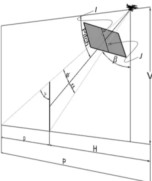
The pinhole model does not consider that real lenses may produce several different non-linear
164
distortions. The major defects in cameras are the radial distortion, caused by the spherical shape of
165
the lens. Other distortions, like the tangential distortion, which is generated when the lens is not
166
parallel to the imaging sensor, have minor relevance and will not be considered in this study. The
167
radial distortions can usually be classified as either barrel distortions or pincushion distortions
168
(Figure 3), are quadratic, meaning they increase as the square of the distance from the center.
169
170
171
172
Figure 3 Effect of barrel and pincushion distortions.
173
Removing a distortion means obtaining an undistorted image point, which can be considered as
174
projected by an ideal pinhole camera, from a distorted image point. The simplest way to model the
175
radial distortion is with a shift to the pixel coordinates. The radial shift of coordinates modifies only
176
the distance of every pixel from the image center. Let 𝑟 represents the observed distance (distorted
177
image coordinates from the center) and 𝑟𝑐𝑜𝑟𝑟 the distance of the undistorted image coordinates from
178
the center. The observed distance for a point in the image plane I of μi and νi coordinates (see
179
Figure 1) can be calculated as follow:
180
𝑟 = √(μi − μ0 )2+ (νi− ν0)2 (11)
With these notations the function that can be used to remove lens distortion is:
181
𝑟𝑐𝑜𝑟𝑟= 𝑓(𝑟) (12)
However, before applying the compensation function 𝑓(𝑟) we need to underline that the
182
model would be useless if images with the same distortion, but different resolutions would have
183
different distortion parameters. Therefore, all pixels should be normalized to a dimensionless frame,
184
where the image resolution is not important. In the dimensionless frame, the diagonal radius of the
185
image is always 1, and the lens center is (0; 0) [25].
186
The formula to transform the pixel coordinates to dimensionless coordinates is the following:
187
188
(𝑝𝑝𝜇 𝜈) = ( (μi − μ0 )/√( 𝑤𝜇 2) 2 + (𝑤𝜈 2) 2 (νi− ν0)/√( 𝑤𝜇 2) 2 + (𝑤𝜈 2) 2 ) (13)189
Where 𝑝𝜇 and 𝑝𝜈 are the dimensionless pixel coordinates and 𝑤𝜇, 𝑤𝜈 are the image width
190
and height in pixels.
191
The dimensionless coordinates defined in (13) can be used to calculate a normalized distance 𝑟𝑝
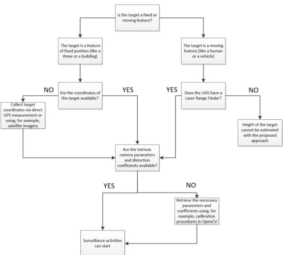
192
considering the formula given in (11). 𝑟𝑝 can be then used to approximate the a normalized 𝑟𝑐𝑜𝑟𝑟
193
with its Taylor expansion [25]:
194
195
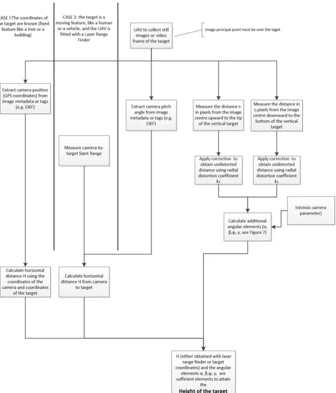
where 𝜅𝑖 are the radial distortion coefficients. The “perfect” approximation would be a
196
polynomial of infinite degree; however, this precision is not needed. Several studies, such as [26],
197
confirmed that for average camera lenses the first order is enough, while more coefficients are
198
required for fish-eye lenses.
199
𝑟𝑐𝑜𝑟𝑟 calculated with (14) needs to be denormalized to obtain the undistorted μi−corr and
200
νi−corr image coordinates for the image under study.
201
202
2.3. Elements to consider when dealing with cameras installed into UAVs operating outdoor
203
204
Several elements need to be taken in due consideration when operating outdoor with cameras
205
installed into UAVs:
206
• The camera is usually fitted into steerable gimbals, which may have the freedom to move
207
along one, two or even three axes (which would be formalistically called one-gimbal,
208
two-gimbal or three-gimbal configurations, [1]). In those cases where the gimbal has
209
limited degrees of freedom, further steering capacity for the camera must be provided by
210
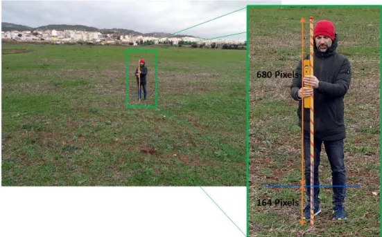
the UAV itself via flight rotations.
211
• The parameters required for the transformation from world coordinate system to camera
212
coordinate (extrinsic parameters) are given by GPS measurements (latitude, longitude, and
213
elevation) and Euler angles (yaw, pitch, and roll). Regular GPS receivers, which are not
214
subject of enhancements such as Differential GPS, may be affected by a relevant positional
215
error, especially in elevation. On the other hand, the orientation angles are measured by
216
sensitive gyroscopes, which usually have very good accuracy [27].
217
• The parameters for the projective transformation from the 3-D camera’s coordinates into
218
the 2-D image coordinates (intrinsic parameters) must be known. For those cases where the
219
UAV camera specs are not available, the intrinsic parameters (image principal point, focal
220
length, and skew) can be retrieved using calibration procedure provided, for example, by
221
computer vision open libraries such as OpenCV [28].
222
• The UAV can orient the camera to have the target centered in the image plane. Besides
223
being a common practice in UAV operations for tracking, is a mandatory requirement for
224
the calculation of height.
225
• The camera is usually oriented in such a way to have the feature of interest centered in the
226
image plane. Tracking algorithms [28] can be used to automatically kept the camera
227
pointed toward the target.
228
• Each video frame or still image acquired by the UAV is usually accompanied by a set of
229
camera and UAV flight information, stored as metadata. The amount of information
230
actually stored varies from system to system. Advanced imaging equipment may provide
231
a complete set of metadata in KLV (Key-Length-Value) format in accordance with MISB
232
(Motion Imagery Standards Board) standards [29]. Lightweight UAV available in the
233
regular market are not always fitted with such advanced devices but, very often, are
234
capable to store a minimum set of metadata which includes on-board GPS coordinates,
235
flight orientation and camera orientation.
236
• Advanced UAV imaging systems are also fitted with laser range finders, which are capable
237
to measure the instantaneous camera-to-target distance and store this information as
238
metadata. The following paragraph describes in details the pinhole model for computer
239
vision analysis and its parameters.
240
241
2.4. Computer vision with cameras installed into UAVs
242
243
The actual camera pose of a “gimballed” optical sensor can be determined through a sequence
244
of homogeneous matrixes defining a number of transformations [30] that can be briefly summarized
245
as follow:
• Transformation from Inertial frame to UAV Vehicle Frame. The UAV vehicle frame is
247
identical to the inertial frame, only translated to the UAV position. This transformation
248
requires a translation which only depends on the UAV’s GPS location and barometric
249
altitude measurements.
250
• Transformation from UAV Vehicle Frame to UAV Body frame: this transformation consists
251
of a single rotation R, based on measurements of Euler angles that define the orientation of
252
the UAV. In aeronautics the Eeuler angles are usually expressed through the yaw (or
253
heading), pitch and roll.
254
• Transformation from UAV Body to Gimbal frame (where the origin of the gimbal frame is
255
the center of the gimbal): this requires a translation which depends on the location of the
256
UAV’s center of mass with respect to the gimbal’s rotation center and a rotation to aligns
257
the gimbal’s coordinates frame with the UAV’s body frame.
258
• Transformation from Gimbal to Camera frame (origin at the camera’s center): this
259
transformation depends on the vector that describes the location of the gimbal’s rotation
260
center relative to the camera center and it is resolved in the camera’s coordinate frame. It
261
also depends on a simple rotation that aligns the camera’s coordinate frame with that of
262
the gimbal.
263
Large UAVs, which are also called MALEs (Medium Altitude Long Enduranc e, [31]), are
264
usually fitted with three-gimbaled advanced imaging systems and accurate positioning systems,
265
such as differential GPS. These systems are capable to calculate all the above-mentioned
266
transformation in real-time and embed the instantaneous camera pose, and other information such
267
as FOV and image footprint on ground, into the acquired video stream using the KLV
268
(Key-Length-Value) encoding protocols [29], in accordance to military standards [32].
269
On the other hand, non-military lightweight UAVs available in the regular market are not
270
always fitted with advanced imaging systems and very accurate GPS. For example, the DJI Phantom
271
4 PRO (a widely diffused multi-rotor platform of 1.388 kg, used to collect data for the testing of the
272
approach described in this paper, see Paragraph 3. Results). is not capable to generate KLV
273
embedded metadata but it can generate ancillary tags in Exchangeable Image File Format (EXIF) of
274
still images which provide, among other information, GPS position of the aircraft, aircraft
275
orientation and camera orientation at the moment of the acquisition of the still image. DJI Phantom 4
276
PRO has a GPS/GLONASS positioning system [33]. The actual accuracy of this positioning system is
277
not specifically indicated by the UAV manufacturer, but it can be roughly assumed between 1m and
278
3m in the condition of good satellite signal [34]. Moreover, it is necessary to underline that the
279
accuracy in altitude of the GPS readings is much lower than the accuracy on the horizontal plane
280
(Latitude, Longitude). The camera of this UAV has a pivoted support (one-gimbal) with a single
281
degree of movement along the Y axis (pitch angle, see Figure 4). Angular values are measured with
282
an accuracy of +/- 0.02° [33]. Although not specified in any available technical documentation but,
283
considering the available information of this UAV, it is here assumed that the transformation
284
employed to provide the information in the EXIF tags are the following: a) the translation defined by
285
the GPS coordinate of the UAV body, b) rotation based on Euler angles of the body followed by c) a
286
1D rotation of the camera (pitch angle). Therefore, the position of the camera when dealing with DJI
287
Phantom 4 PRO can be defined by UAV body positional location (GPS coordinates) while the
288
orientation is given by a yaw angle defined by flight orientation, a pitch angle defined by camera
289
orientation and a roll angle defined by flight orientation.
290
The camera sensor is a CMOS of 20M effective pixels with 5472 x 3648 resolution and 13.2 x
291
8.8mm size, lens focal length of 8.8 mm with no optical zoom and FOV of 84°.
292
293
294
Figure 4 Axis and Euler angles for the case of DJI Phantom 4 PRO.
295
Let’s now assume to have a lightweight UAV, like the one descripted in Figure 4, and a feature
296
standing vertically on the ground, for example a pole. Let’s also assume that the UAV has a heading
297
(Yaw angle) and pitch angle appropriate to pointing to the target as graphically represented in
298
Figure 5. Let’s also assume that the roll angle is equal to zero 0.
299
300
301
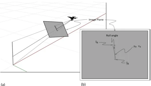
Figure 5 graphical representation of a lightweight UAV pointing to a vertical pole (a) with Roll angle equal to
302
zero. In (b) the image plane is represented in orthogonal view (as it would appear on screen).
303
Point μ0, ν0 in Figure 5b is the camera center, which is obtained, as already described, by the
304
interception between the image plane and the optical axis (see Figure 5a). The optical axis is centered
305
to the target, not necessarily the midpoint but any point of the pole. The Image Point I is given by the
306
interception of the camera ray line that connects the tip (highest point) of the pole with the camera
307
center. This point is expressed by the image coordinate μi, νi while 𝑟̂𝑖 represents the distance from
308
the image center. Moreover, 𝑟̂𝑖 is a distorted value that needs to be compensated to obtain the
309
distance ri−corr of the ideal undistorted image. The procedure to obtain such undistorted distance
310
was already discussed in the previous paragraph (see (14). Similarly, the Image Point J is the
311
interception of the image plane with the ray line that connects the bottom of the pole (lowest point)
with the camera center. The point is expressed by the image coordinate μj, νj while 𝑟̂𝑗 represents the
313
distance from the image center that needs to be compensated to get rj−corr, the undistorted distance
314
from the center of the ideal undistorted image. The line I-J in the image plane is the height of pole
315
expressed in pixels in the image plane.
316
Let’s now consider the same case when the Roll angle is different than zero, as graphically
317
represented in Figure 6.
318
319
320
Figure 6 graphical representation of a lightweight UAV pointing to a vertical pole (a) with Roll angle different
321
than zero. Orthogonal view of the image plane (b) with the representation of the pole and indication of the Roll
322
angle.
323
When the Roll angle is different than zero, the line IR-JR, which is the representation of the pole
324
in the image plane, will not appear as parallel to the ν axes, as in the case before, but rotated of an
325
angle equal to the Roll angle itself, as it possible to infer from (7). As mentioned above, the observed
326
distances (respectively 𝑟̂𝑅𝑖 and 𝑟̂𝑅𝑗) must be compensated to obtain the distances rRi −corr and
327
rRj−corr of the ideal undistorted image.
328
The next paragraph describes how to estimate the height of a target standing vertically (pole)
329
considering the elements discussed so far in this paper. It is used, as an example, a lightweight UAV
330
like the DJI Phantom 4 PRO but the approach can be extended to any imaging system installed in
331
steerable moving platforms.
332
2.5. Estimating target height with camera fitted into UAVs
333
The approach proposed in this study for the estimation of target height using camera fitted into
334
UAVs foresees the UAV pointing at the target as depicted in Figure 5 and Figure 6. Let’s get started
335
with the case when the roll is zero (see Figure 7).
336
337
338
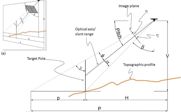
339
340
Figure 7 Perspective view of a lightweight UAV pointing to a vertical target (pole) (a). Orthogonal view of the
341
same scene with descriptions (b).
342
The pitch angle, which can be also identified with 𝜃𝑦, see (9) is a known value, while the angles
343
𝛼 , 𝛽 , 𝜙 , 𝛾 are not originally known but they can be retrieved using simple trigonometric
344
calculations:345
𝛼 = tan−1(𝑟𝑗−𝑐𝑜𝑟𝑟 𝐹 ) (15) 𝛽 = 90 − (𝜃𝑦+ 𝛼) (16) 𝜙 = tan−1(𝑟𝑖−𝑐𝑜𝑟𝑟 𝐹 ) (17) 𝛾 = ( 𝜙 + 𝛽 + 𝛼) (18)Where 𝑟𝑖−𝑐𝑜𝑟𝑟 can be calculated considering (14) in the previous paragraph starting from the
346
observed 𝑟𝑖 in the image plane (see Figure 7). Similarly, 𝑟𝑗−𝑐𝑜𝑟𝑟 referrers to the point J (see also
347
Figure 5). F is the focal length, which was defined by (3) and (4) (assumed here for simplicity that
348
𝐹 = 𝐹ν= 𝐹μ).
349
V in Figure 7 is the vertical distance between the base of the target and the camera center, while
350
H is the horizontal distance between the target and the camera center. To be underlined H and V are
351
not related at all to the topography, as it possible to infer in Figure 7. If the coordinates of the target
352
are known, then H and V are also known since the GPS coordinate of the camera are available (see
353
Paragraph 2.3. Cameras installed into UAVs). The accuracy of the GPS and how it will impact the
354
estimation of the target height will be treated later in this paper, but, since the accuracy of altitude in
355
the GPS readings is much lower than the accuracy on the horizontal plane (Latitude, Longitude), V is
356
always calculated in function of H, as defined in (19) below.
𝑉 = 𝐻 tan(90 − 𝛽) (19) the angles 𝛼, 𝛽, 𝜙, 𝛾 are now known, as well as the pitch angle, V and H. These elements can
358
be used to calculate the height of the target using the triangles similarity theorem. In fact, P (see
359
Figure 7) can be calculated as follow:
360
𝑃 = 𝑉 tan(𝛼 + 𝛽 + 𝜙) (20)
p is which is the horizontal distance between the base of the target and the camera ray that
361
passes thought the tip (highest point) of the target, which can be calculated as follow:
362
𝑝 = 𝑃 − 𝐻 (21)
Finally, the height of the target can be calculated:
363
𝐻𝑒𝑖𝑔ℎ𝑡 𝑜𝑓 𝑡ℎ𝑒 𝑇𝑎𝑟𝑔𝑒𝑡 = 𝑝 tan(90 − 𝛾) (22)
As already mentioned, the horizontal distance between the target and the camera center can be
364
determined if the coordinates of the target are known. In practice, this could be the case only when
365
dealing with immobile features like trees or buildings. If the position of the target is not known, as it
366
may happen for moving targets like humans, vehicles, etc., laser range finder devices can be used to
367
measure the instantaneous camera-to-target distance (slant range). As already mentioned, advanced
368
imaging systems are very often fitted with such devices [1] and the instantaneous distance
369
measurements can be stored in the KLV metadata set [31].
370
Slant Range values are distance is aligned to the optical axis of the camera (see Figure 7) and
371
used to calculate the horizontal distance H using the following formula:
372
𝐻 = 𝑆𝑙𝑎𝑛𝑡 𝑅𝑎𝑛𝑔𝑒 𝐷𝑖𝑠𝑡𝑎𝑛𝑐𝑒 ∗ sin(90 − 𝑃𝑖𝑡𝑐ℎ 𝑎𝑛𝑔𝑙𝑒) (23)
373
To be underlined that also the Slant Range distances measured by laser range finders are
374
affected by a certain error that should duly be considered during the estimation of target height.
375
376
Let’s now analyze the case when the roll angle is different than zero. In this case, as already
377
discussed (see Figure 6) the points Iand J are not located along the υ axis passing on the center of the
378
image. In other words, a vertical feature will appear as “tilted” in the image on an angle equal to
379
Roll. However, as it possible to infer from (10) and as graphically represented in Figure 8, I and J are
380
in the same (vertical) plane than Pitch angle. In other words, the approach presented in this paper
381
does not need to consider the Roll angle for the calculation of target height. Also, in this case it is
382
necessary to perform distortion correction to obtain 𝑟𝑖−𝑐𝑜𝑟𝑟 and 𝑟𝑗−𝑐𝑜𝑟𝑟 and use these parameters in
383
the formulas previously described (see (15) and (17)).
385
386
Figure 8 Perspective view of the image plane with visualization of the I and J, representing respectively the top
387
and the bottom of the pole in the mage plane.
388
2.6. Workflows for target height estimation
389
390
The approach described in the following paragraphs is here summarized through workflows
391
which are intended to be of practical use. The first workflow in Figure 9 should be considered
392
during the planning phase prior to initiate a surveillance campaign to define if all the condition to
393
estimate the height of the target feature are in place. It is necessary to underline that if the target is a
394
moving feature and the UAV is not equipped with a laser range finder, it would not be possible to
395
estimate the height of the target with the proposed procedure. This is relevant limitation should be
396
addressed in future studies. The second workflow (Figure 10) describes the actions to perform
397
during the UAV flight to obtain all the information needed to calculate feature height.
398
399
400
Figure 9 Workflow to verify if all the conditions to estimate the height of the target feature are in pl ace. This
401
analysis should be done during the planning phase prior to initiate a surveillance campaign.
402
403
404
405
Figure 10 Workflow describing the actions to perform during the UAV flight to obtain all the information
406
needed to calculate feature’s height.
407
3. Results
408
The procedure to estimate target height described in the previous section was tested using real
409
data acquired with a DJI Phantom 4 PRO (see Paragraph 2.3. Cameras installed into UAVs for
410
technical details regarding this device and camera used). In this field test it was used as target a
411
wooden pole of 180 cm standing vertically from ground located in a position of known coordinates.
412
32 still images were acquired with different camera poses and, in each acquired image, the principal
413
point was always oriented over the pole (any point along pole as defined in Figure 6). Images not
414
properly oriented (principal point not located over the pole) were discarded and not used in this
415
study. The images were acquired in an open space with good visibility to satellites.
GPS readings (position of the UAV in WGS84 geographic coordinates) and camera pitch angle
417
of each image were extracted from EXIF tags while the number of pixels spanning upward from
418
image principal point (𝑟𝑖) and downward (𝑟𝑗) were measured manually on screen (see also Figure
419
11). The Lat-Long coordinates of each image were plotted into a GIS environment along with the
420
position of the reference pole to measure horizontal distance (H values, as graphically described in
421
Figure 7). The first part of the Table 1 and Table 2 provides the above-discussed data for all the
422
acquired images.
423
424
425
Figure 11 Still image acquired with DJI Phamtom 4 PRO with image principal point (visualized in the picture
426
with a blue cross) located over the pole. The number of pixels spanning upward (680) and downward (164)
427
from the image principal point were measured manually on screen. A level of 0.4m length was kept tight and
428
alight to the pole to maintain it vertical during the acquisition of each shot.
429
As mentioned in the previous paragraph, the GPS readings have an accuracy between 1 to 3m.
430
An accuracy of 1m means that the real position of the UAV is not known, but it must be located (with
431
a probability of 95%) within a circle of 0.5 radius around the GPS readings given in the EXIF tag.
432
Therefore, the distance of the UAV from the pole could be any value within H+0.50m and H-0.50m.
433
In Table 1 and Table 2 this element has been reported as H+GPS Err and H-GPS Err for each image.
434
The accuracy of the angular measurement is +/- 0.02° (see Paragraph 2.3. Cameras installed into
435
UAVs), which is neglectable for the purpose of this study.
436
In the paragraph 2.2 it was described the procedure to obtain a corrected distance from image
437
center. Such a procedure was applied to each image obtaining the 𝑟𝑖−𝑐𝑜𝑟𝑟 (number of corrected
438
pixels from image center upward to pole’s top point) and 𝑟𝑗−𝑐𝑜𝑟𝑟 (number of corrected pixels from
439
image center downward to pole’s bottom). These values, as well as the total number of pixels
440
spanning the entire pole, are reported in Table 1 and Table 2. The Distortion Coefficient to be used
441
for the correction was retrieved through camera calibration techniques [20] developed with OpenCV
442
via Python programming.
443
The calculation of the target height (pole) was performed in accordance with the procedure
444
described in the Paragraph 2.4. Target height (NO GPS err) in Table 1 and Table 2 indicates the
445
estimated height of the pole considering the Horizontal distance considering the camera position
446
indicated in the EXIF tags. On the other hand, Target height (when H+ GPS err) and Target height (when
447
H- GPS err) in Table 1 and Table 2 provide the calculated height of the pole considering a GPS error
448
of +/- 0.5m).
The field called Height Uncertainty in Table 1 and Table 2 represents the arithmetical difference
450
between Target height (when H+ GPS err) and Target height (when H- GPS err).
451
452
Sensors 2019, 19, x; doi: FOR PEER REVIEW www.mdpi.com/journal/sensors
453
Table 1 data and results for the first 16 still images acquired with the lightweight UAV.
454
DJI31 DJI32 DJI34 DJI41 DJ09 DJI12 DJI13 DJI15 DJI17 DJI18 DJI33 DJI35 DJI36 DJI37 DJI42 DJI_125 DJI42 Number of pixels upwards (ri) 355 680 172 151 1358 1352 942 931 592 363 678 150 334 344 156 154 156
Number of pixels downwards (rj) 1150 164 204 142 49 69 82 92 48 61 160 216 203 514 141 297 141
Gimbal pitch angle (degrees) 13.7 13.7 5.6 14.8 38.7 38.7 26.4 26.4 16 10.1 13.7 12 17.9 30.6 14.8 26.7 14.8 Flight roll angle (degrees) 1.8 0.9 4.2 5.2 0.4 0.8 0.5 0 0.6 0.3 1.2 2.9 3.3 0.8 1.3 3.6 1.3 Horizontal distance (H) (m) 4.2 7.9 17.1 21.28 3.6 3.64 6.04 6.17 10.28 14.96 7.95 17.38 11.62 6.04 21.12 11.78 21.12
H+ GPS err (m) 4.7 8.4 17.6 21.78 4.1 4.14 6.54 6.67 10.78 15.46 8.45 17.88 12.12 6.54 21.62 12.28 21.62 H- GPS err (m) 3.7 7.4 16.6 20.78 3.1 3.14 5.54 5.67 9.78 14.46 7.45 16.88 11.12 5.54 20.62 11.28 20.62
ri-corr (upward) in pixels 355 679 172 151 1352 1346 940 929 591 363 677 150 334 344 156 154 156
rj-corr (downward) in pixels 1146 164 204 142 49 69 82 92 48 61 160 216 203 514 141 297 141
Total number of pixels 1501 843 376 293 1401 1415 1022 1021 639 424 837 366 537 858 297 451 297
Target height (NO GPS err) (m) 1.94 1.87 1.78 1.83 1.77 1.82 1.89 1.93 1.87 1.77 1.87 1.83 1.87 1.98 1.84 1.87 1.84 Target height (when H+ GPS err) 2.17 1.99 1.84 1.88 2.01 2.07 2.05 2.09 1.96 1.83 1.99 1.88 1.95 2.14 1.88 1.94 1.88 Target height (when H- GPS err) 1.71 1.75 1.73 1.79 1.52 1.57 1.73 1.78 1.78 1.71 1.75 1.78 1.79 1.82 1.79 1.79 1.79 Uncertainty (m) 0.46 0.24 0.10 0.09 0.49 0.50 0.31 0.31 0.18 0.12 0.23 0.11 0.16 0.33 0.09 0.16 0.19
455
456
457
458
459
460
461
Table 2 data and results for the remaining 16 still images acquired with the lightweight UAV (continuation of Table 1).
462
DJI143 DJI144 DJI148 DJI149 DJI150 DJI151 DJI152 DJI153 DJI154 DJI155 DJI156 DJI157 DJI40 DJI43 DJI137 Number of pixels upwards (ri) 207 359 32 83 68 112 241 156 307 339 573 902 254 114 136
Number of pixels downwards (rj) 208 75 86 26 102 90 145 78 304 280 559 211 180 161 33
Gimbal pitch angle (degrees) 38.5 39.4 6.9 16.6 30.4 47.3 20.7 10.7 34.4 34.4 34.5 41.7 22.9 22.4 15.5 Flight roll angle (degrees) 9.6 8.5 5.5 8.6 3.1 3 3.8 5.2 3.3 4.2 2.8 7.1 1.9 1.1 5.6 Horizontal distance (H) (m) 9.51 9.71 54.24 54.49 28.33 15.33 14.85 26.68 7.43 7.3 4.22 4.13 13.38 21.08 37.12
H+ GPS err (m) 10.01 10.21 54.74 54.99 28.83 15.83 15.35 27.18 7.93 7.8 4.72 4.63 13.88 21.58 37.62 H- GPS err (m) 9.01 9.21 53.74 53.99 27.83 14.83 14.35 26.18 6.93 6.8 3.72 3.63 12.88 20.58 36.62
ri-corr (upward) in pixels 207 359 29 83 68 112 241 156 307 339 573 900 254 114 136
rj-corr (downward) in pixels 208 75 84 26 102 90 145 78 304 280 559 211 180 161 33
Total number of pixels 415 434 118 109 170 202 386 234 611 619 1132 1111 434 275 169
Target height (NO GPS err) (m) 1.79 1.84 1.79 1.78 1.79 1.84 1.78 1.77 1.83 1.81 1.95 1.96 1.86 1.87 1.85 Target height (when H+ GPS err) 1.89 1.93 1.81 1.80 1.82 1.90 1.84 1.80 1.96 1.93 2.18 2.20 1.93 1.91 1.87 Target height (when H- GPS err) 1.70 1.75 1.77 1.77 1.75 1.78 1.72 1.74 1.71 1.69 1.72 1.73 1.79 1.82 1.82 Uncertainty (m) 0.19 0.19 0.03 0.03 0.06 0.12 0.12 0.07 0.25 0.25 0.46 0.48 0.14 0.09 0.05
463
464
465
466
Sensors 2019, 19, x; doi: FOR PEER REVIEW www.mdpi.com/journal/sensors
Looking at Target height (NO GPS err) in Table 1 and Table 2, the results clearly indicate that in
467
almost no image the correct height (180cm) is obtained. However, considering Target height when H+
468
GPS err and Target height (when H- GPS err), which give interval from the highest and lowest possible
469
height value considering the GPS error, we can see that 180cm is (almost) always within the range of
470
each image. This can be also visualized in Figure 12. Only the images DJI137, DJI43 and DJI137 don’t
471
include the real value (1.80m) within their range, assuming a GPS error of +/- 0.5m.
472
In other words, the accuracy in the estimation of target height depends on the error associated
473
to the horizontal distance H. In a real case scenario, taking for example the case of the image DJI143
474
(first column on Table 2), we could only say that the real height of the target has a value included
475
between 1.70m and 1.89m (0.19m interval).
476
477
478
Figure 12 Grey rhombus represent the target height calculated considering GPS reading extracted from the
479
EXIF tags for each acquired image, while the vertical lines represent the uncertainty when GPS error is 1m.
480
Let’s now analyze the case when GPS is assumed to be 3m (the results of this analysis are not
481
ere reported in a tabular format but only graphically in Figure 13). The first element to notice is that
482
the accuracy intervals have greatly increased, for example for DJI143 the real value may range
483
from1.51m to 2.08m (0.57m interval), three times bigger than the interval obtained when the
484
horizontal accuracy was assumed to be 1m. The second element to underline is that all the images
485
have the real height value (1.80m) included in their interval. Even those images that did not have the
486
right height within their interval assuming a positional accuracy of 1m (DJI137, DJI43 and DJI137).
487
This simply means that the positional accuracy of those three images is more than 1m and below 3m.
488
In the case here under discussion the horizontal distance was calculated considering the
489
coordinates of the target and UAV. A similar approach should be also considered when dealing with
490
slant-range measurements obtained with laser range finders installed into UAVs. These devices may
491
measure distances with a certain error that, taking into the account (23), generate uncertainty in the
492
correct estimation of target height, as seen for the case above.
493
494
1.50 1.60 1.70 1.80 1.90 2.00 2.10 2.20 D J0 9 D JI 1 2 D JI 1 2 5 D JI 1 3 D JI 1 3 7 D JI 1 4 2 D JI 1 4 3 D JI 1 4 4 D JI 1 4 8 D JI 1 4 9 D JI 1 5 D JI 1 5 0 D JI 1 5 1 D JI 1 5 2 D JI 1 5 3 D JI 1 5 4 D JI 1 5 5 D JI 1 5 6 D JI 1 5 7 D JI 1 7 D JI 1 8 D JI 3 1 D JI 3 2 D JI 3 3 D JI 3 4 D JI 3 5 D JI 3 6 D JI 3 7 D JI 4 0 D JI 4 1 D JI 4 2 D JI 4 3495
Figure 13 Grey rhombus represent the target height calculated considering GPS reading extracted from the
496
EXIF tags for each acquired image, while the vertical lines represent the uncertainty when GPS error is 3m.
497
We should also notice in Figure 12 and Figure 13 that the uncertainty is not constant, but it
498
rather changes substantially from image to image. An uncertainty analysis can be conducted using
499
the data described in Table 1 and Table 2 to verify how the parameters involved in the calculations
500
are affecting the uncertainty.
501
The first parameter to consider is the Pitch angle. However, this parameter may depend on
502
which part of the vertical target the camera is pointing to (see Figure 7). To avoid this issue, it is
503
preferable to consider the Pitch angle plus α angle, in this way we always refereeing to the bottom
504
point of the pole in every image. In Figure 14 the angles obtained by the Pitch angle plus the α angle
505
are plotted against the Height Uncertainty values of the images described in Table 1 and Table 2
506
(horizontal accuracy of 1m). The data distribution looks quite sparse although we may say that the
507
uncertainty is generally growing when the Pitch angles are higher, as the best linear fit and its
508
coefficient of determination can also attest.
509
The second parameter to consider is the camera-to-target horizontal distance H. If we plot in a
510
graph the uncertainty against the horizontal distance, we can notice a clear relationship between
511
them (see Figure 15). They are related by an exponential relationship which tells us that the accuracy
512
is lower when the horizontal distance is higher. In Figure 15 it is reported the equation of the curve
513
that best fits when the horizontal accuracy of 1m.
514
The distance from the image center to top and bottom of the pole measure in pixels after
515
distortion correction (𝑟𝑖−𝑐𝑜𝑟𝑟 and 𝑟𝑗−𝑐𝑜𝑟𝑟) should be also considered. However, as seen for the Pitch
516
angle, also these parameters depend on which part of the vertical target the camera is pointing to. It
517
is therefore preferable to consider the total number of pixels spanning the feature (the pole) for this
518
analysis. In Figure 16 the Total Number of Pixels for each image was plotted against the Height
519
Uncertainty. The data distribution shows a quite evident linear trend, the equation of the best linear
520
fit and its coefficient of determination are also reported in the figure.
521
Finally, intrinsic camera parameters should be also considered to analyze how they influence
522
the overall accuracy. This analysis was not performed in this study because all the images were
523
acquired with the same camera configuration.
524
1 1.2 1.4 1.6 1.8 2 2.2 2.4 2.6 D J0 9 D JI 1 2 D JI 1 2 5 D JI 1 3 D JI 1 3 7 D JI 1 4 2 D JI 1 4 3 D JI 1 4 4 D JI 1 4 8 D JI 1 4 9 D JI 1 5 D JI 1 5 0 D JI 1 5 1 D JI 1 5 2 D JI 1 5 3 D JI 1 5 4 D JI 1 5 5 D JI 1 5 6 D JI 1 5 7 D JI 1 7 D JI 1 8 D JI 3 1 D JI 3 2 D JI 3 3 D JI 3 4 D JI 3 5 D JI 3 6 D JI 3 7 D JI 4 0 D JI 4 1 D JI 4 2 D JI 4 3525
Figure 14 Pitch angle plus α angle expressed in degrees (y) vs uncertainty values expressed in meters (x) for the
526
images described in Table 1 and Table 2. The equation of the best linear fit and its coefficient of determination
527
are also reported.
528
529
530
Figure 15 Horizontal distance expressed in meters (y) vs uncertainty values expressed in meters (x) for the
531
images described in Table 1 and Table 2. The equation of the best exponential fit curve and its coefficient of
532
determination are also reported.
533
y = 0.0058x + 0.045 R² = 0.2925 0 0.1 0.2 0.3 0.4 0.5 0.6 0 10 20 30 40 50 60 70Pitch angle + α angle vs height uncertainty
y = 1.9604x-1.026 R² = 0.9986 0.0 0.1 0.2 0.3 0.4 0.5 0.6 0 10 20 30 40 50 60
534
Figure 16 Total Number of Pixels (y) vs uncertainty values expressed in meters (x). The equation of the best
535
linear fit and its coefficient of determination are also reported.
536
The graph in Figure 15 is particularly interesting. The regression curve has an extremely good
537
coefficient of determination to the data; therefore, the equation of the curve can tell us quite precisely
538
which is the expected accuracy considering a certain distance from the target.
539
540
Although not directly related to uncertainty analysis, it is also interesting to analyze the
541
correlation between Total Number of Pixels and the Horizontal Distance, this is shown in Figure 17.
542
The data distribution can be well fitted with a power regression curve, whose equation and
543
coefficient of determination are reported in the graph. This relationship is valid for a target of 1.80m,
544
which was the height of the pole used in this study; further research should be conducted to verify if
545
there is a clear and well predictable relationship also for different target heights. If this is the case,
546
the target-to-target distance could be no longer a required parameter for the calculations. The
547
relationship shown in Figure 17 also explains the linear correlation between Height Uncertainty and
548
Total Number of Pixels seen in Figure 16. On the other hand, there is no evident relationship
549
between pith angle and number of pixels as shown in Figure 18.
550
551
y = 0.0003x + 0.0081 R² = 0.9098 0.0 0.1 0.2 0.3 0.4 0.5 0.6 0 200 400 600 800 1000 1200 1400 1600552
Figure 17 Total Number of Pixels (y) vs horizontal distance expressed in meters (x) for the images described in
553
Table 1 and Table 2. The equation of the best regression curve and its coefficient of determination are also
554
reported in the figure.
555
556
557
Figure 18 Total number of pixels (y) vs Pitch angle expressed in degrees (x) for the images described in Table 1
558
and Table 2. The equation of the best linear fit and its coefficient of determination are also reported.
559
Finally, it is interesting to analyze the impact of an inaccurate distortion correction. A
560
non-accurate correction, that may lead to an erroneous value of the distance from the image center
561
measured in pixels. Therefore, it is important to understand how a variation of number of pixels
562
may impact the estimation of the target height. To achieve this goal, 5 pixels were added to the total
563
number of pixels (3 upward and 2 downward, the values were chosen arbitrary) and the height was
564
recalculated to verify the variation. The results are reported in Table 3.
565
The difference in height varies from 0.005m up to 0.08m, and it increases linearly with the
566
horizontal distance, as we may expect. This analysis demonstrates that a non-accurate distortion
567
correction may lead to an erroneous value of height, which is however much lower than the error
568
associated to the horizontal distance. This statement is anyway true for the camera and UAV system
569
used in this study; other cameras with a different resolution may give different errors.
570
y = 4443.3x-0.928 R² = 0.8552 0 200 400 600 800 1000 1200 1400 1600 0 10 20 30 40 50 60Total number of pixels vs horizontal Distance (H)
y = 5.7841x + 445.08 R² = 0.0354 0 200 400 600 800 1000 1200 1400 1600 0 10 20 30 40 50 60 70
571
Table 3 The height calculated with the number of pixels measured in each image is compared with height
572
calculated by adding 5 pixels to the original number. The table reports also the difference between the height
573
calculated with the original number the height with when 5 pixels are added.