Deteção de fraude em telecomunicações com técnicas de Data Mining

U

P

F

E

Deteção de Fraude em

Telecomunicações com Técnicas de Data

Mining

João Vitor Cepêda de Sousa

Master in Electrical and Computers Engineering

Supervisor: Prof. Dr. Carlos Manuel Milheiro de Oliveira Pinto Soares Co-Supervisor: Prof. Dr. Luís Fernando Rainho Alves Torgo

c

•

PORTO

crUDFACULOADE DE ENGENHARIA

• E— I~ UNIVERSIDADE DO PORTO

A Dissertação intitulada

“Deteção de Fraude em Telecomunicações com Técnicas de Data Mining”

foi aprov&da em provas realizadas em 25-07-2014

o júri

Presidente Professora Doutora Maria Teresa Magalhâes da Silva Pinto de Andrade

Professora Auxiliar do Departamento de Engenharia Eletrotécnica e de

c

outor

Auxit nformática do Universidade do Minho

&~

Professor Doutor Carlos Manuel Milheiro de Oliveira Pinto Soares

Professor Associado do Departamento de Engenharia Informática da Faculdade de Engenharia da Universidade do Porto

O autor declara que a presente dissertação (ou relatório de projeto) é da sua exclusiva autoria e foi escrita sem qualquer apoio externo não explicitamente autorizado. Os resultados, ideias, parágrafos, ou outros extratos tomados de ou inspirados em trabalhos de outros autores, e demais referências bibliográficas usadas, são corretamente citados.

~

c

Autor -

João Vitor Cepeda de Sousa

Abstract

This document presents the final report of the thesis “Telecommunication Fraud Detection Using Data Mining Techniques”, were a study is made over the effect of the unbalanced class data, generated by the Telecommunications Industry, in the performance of the classification algorithm Naive Bayes. In this subject, an unbalanced class data set is characterized by an uneven class distribution where the amount of fraudulent instances (positive class) is substantially smaller than the amount normal instances (negative class). This will result in a classifier which is most likely to classify data belonging to the normal class then to the fraud class. At first, an overall inspection is made over the data characteristics and the Naive Bayes model. A feature engineering stage is executed, with the intent to extend the information contained in the data creating a depper relation with the data itself and algorithm characteristics. A previously proposed solution that consists on undersampling the most abundant class (normal) before building the model, is presented and tested. In the end, the new proposals are presented. The first proposal is to study the effects of changing the intrinsic class distribution parameter in the Naive Bayes model and evaluate its performance. The second proposal consists in estimating margin values that when applied to the model output, attempt to bring more positive instances from previous negative classification. All of these suggested models are validated over a monte-carlo experiment, using data with and without the engineered features.

Acknowledgements

My first words of acknowledgment must be to my mother, Olimpia Cepêda, for the love and patient she offered me during my path to become an engineer. She always supported all of my choices and gave me strength to endure it all. I thank her for all the work I gave her during my growing up and I hope to later on help her as much as she did me.

A big and lovely thanks to my woman, Tânia Trindade. Without her love it would be harder to support the long hours of work without breaking. She had the patient and the happiness to cheer me when I was down and to be behind my back when I need it. I hope to be there for all her hard times.

I would also like to thank my supervisor, Carlos Soares, and co-supervisor, Luís Torgo, for all the help and advisement they gave me during this work. In a more funny way to describe it, I thank for all the patient that they have showed when I asked my thousands of silly questions. I will attempt to be there for your assistance when you need or request it.

To finish, I also like to thank my friends for the support, and my laptop for not giving up on my thousand hour’s data processing marathons!

Thank you!

João Cepêda

“Prediction is very difficult, especially if it’s about the future.”

Niels Bohr

Contents

2 State Of the Art 5 2.1 Telecommunications Fraud . . . 5 2.1.1 Historical Remarks . . . 5 2.1.2 Fraud Methods . . . 7 2.2 Anomaly Detection . . . 8 2.2.1 Anomaly Types . . . 9 2.2.2 Data Mining . . . 10 2.2.3 Learning Types . . . 11 2.2.4 Model Evaluation . . . 12

2.3 Data Mining Techniques for Anomaly Detection . . . 14

2.3.1 Clustering based techniques . . . 14

2.3.2 Nearest neighbour based techniques . . . 15

2.3.3 Statistical Techniques . . . 15

2.3.4 Classification Techniques . . . 16

2.3.5 Classification with Unbalanced Datasets . . . 17

2.4 Data Mining on Fraud Detection . . . 17

2.4.1 Data Format . . . 17

2.4.2 User Profiling . . . 18

2.4.3 Rule based applications . . . 18

2.4.4 Neural networks Applications . . . 19

2.4.5 Other Applications . . . 19

3 Naive Bayes 21 3.1 Algorithm . . . 21

3.1.1 Naive Bayes for Classification . . . 22

3.1.2 LaPlace Correction . . . 22

3.1.3 Continuous Variables . . . 23

3.2 Previous adaptations . . . 23

3.3 Proposal . . . 24

3.3.1 Naive Class Distribution . . . 24

3.3.2 Naive Bayes Margin . . . 25

x CONTENTS

4 Prediction of Telecom Anomalies 29

4.1 Data Understanding . . . 29

4.2 Data Preparation . . . 33

4.3 Methodology . . . 34

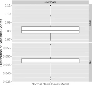
4.4 Results . . . 37

4.4.1 Normal Naive Bayes Results . . . 37

4.4.2 Undersampled Naive Bayes Results . . . 38

4.4.3 Prior Naive Bayes Results . . . 42

4.4.4 Maximal Positive Margin Naive Bayes Results . . . 44

5 Conclusions 47 5.1 Future Work . . . 48

List of Figures

2.1 Blue Box Device . . . 7

2.2 2013 WorldWide Telecommunications Fraud Methods Statistics. . . 8

2.3 Outliers example in a bidimensional data set. . . 9

2.4 2 models ROC curve Comparison . . . 13

3.1 Standard Naive Bayes model construction squematics . . . 25

3.2 Naive Class Distribution model construction squematics . . . 26

3.3 Naive Bayes Margin model construction squematics . . . 27

4.1 Class distribution in each day . . . 31

4.2 Number of calls per hour in each day . . . 31

4.3 Number of calls by duration in day 1 . . . 32

4.4 Number of calls by duration in day 2 . . . 32

4.5 Call Classification Simulation Process . . . 35

4.6 Normal Naive Bayes Model . . . 35

4.7 Undersample Naive Bayes Model . . . 36

4.8 Prior Naive Bayes Model (Naive Class Distribution proposal) . . . 36

4.9 Maximal Positive Margin Naive Bayes Model (Naive Bayes Margin proposal) . . 36

4.10 Normal Naive Bayes model using data without signature . . . 38

4.11 Normal Naive Bayes model using data with signature of type 1 . . . 38

4.12 Normal Naive Bayes model using data with signature of type 2 . . . 38

4.13 Undersampled Naive Bayes model using data without signature . . . 39

4.14 Undersampled Naive Bayes model using data with signature of type 1 . . . 39

4.15 Undersampled Naive Bayes model using data with signature of type 2 . . . 39

4.16 Undersampled Naive Bayes model using data without signature (1% to 10% un-dersampling rate) . . . 40

4.17 Undersampled Naive Bayes model using data with signature of type 1 (1% to 10% undersampling rate) . . . 40

4.18 Undersampled Naive Bayes model using data with signature of type 2 ( 1% to 10% undersampling rate) . . . 40

4.19 Undersampled Naive Bayes model F1 Score (1% to 10% range) . . . 41

4.20 Undersampled Naive Bayes model F1 Score (10% to 100% range) . . . 41

4.21 Prior Naive Bayes model using data without signature . . . 42

4.22 Prior Naive Bayes model using data with signature of type 1 . . . 42

4.23 Prior Naive Bayes model using data with signature of type 2 . . . 43

4.24 Prior Naive Bayes model F1 Score . . . 43

4.25 Maximal Positive Margin Naive Bayes model using data without signature . . . . 44

4.26 Maximal Positive Margin Naive Bayes model using data with signature of type 1 44

xii LIST OF FIGURES

4.27 Maximal Positive Margin Naive Bayes model using data with signature of type 2 44

4.28 Normal Naive Bayes Model ROC Curve . . . 45

List of Tables

1.1 Annual Global Telecommunications Industry Lost Revenue . . . 1

2.1 Frequency-Digit correspondence on the Operator MF Pulsing . . . 6

4.1 Amount of converted positive intances and their corresponding label. . . 45

Abbreviations

ASPeCT Advanced Security for Personal Communications Technologies

CDR Call Details Record

CFCA Communications Fraud Control Association

DC-1 Detector Constructor

LDA Latent Dirichlet Allocation

MF Multiple-Frequency

SIM Subscriber Identity Module

SMS Short Message System

SOM Self-Organizing Maps

SVM Support Vector Machine

Chapter 1

Introduction

1.1

Motivation

Telecommunications fraud is one of the major concerns in the telecommunications industry and corresponds to the abusive usage of an operator infrastructure. This means that a third party is using the resources of a carrier without the intention of paying them. This problem results in significal damages in the financial field [1] since fraudsters are currently stealling part of the revenue of the operators who offer these type of services [2,3]. Others aspects of the problem that causes loss of revenue, are the use of the identity of legitimate clients in order to commit fraud, which result in those clients being framed for a fraud attack that they didn’t commit. This will result in the loss of confidence of the client in their carrier, giving them reasons to leave. Besides being victims of fraud, some clients just don’t like to work with a carrier who has been victim of fraud attacks. Since the offering of the same services is available by multiple carriers, the client can always switch very easily between them [4].

2005 2008 2011 2013 Estimated Global Revenue (USD) 1.2 Trillion 1.7 Trillion 2.1 Trillion 2.2 Trillion

Lost Revenue to Fraud (USD) 61.3 Billion 60.1 Billion 40.1 Billion 46.3 Billion % Representativa 5.11% 3.54% 1.88%

Table 1.1: Annual Global Telecommunications Industry Lost Revenue

Table1.1displays the dimension of the "financial hole" generated by fraud in the telecommu-nications industry and the impact of fraud in the annual revenue of the operators.

There are a couple of reasons which make the fraud in this area appealing for some fraudsters. One is the difficulty in the tracking of the fraudster. This is very expensive process and requires a lot of time, which makes it impractical to detect a large amount of individuals. Another reason is the technological requirements to commit fraud in these systems. A fraudster doesn’t require a particularly sophisticated equipment in order to practice fraud in these systems [5].

All these evidences generate the need to detect the fraudsters in the most effective way in order to avoid future damage to the telecommunications industry.

2 Introduction

Data mining techniques are one possible solution, since they allow the identification of fraud-ulent activity with a certain degree of confidence. Data mining also works specially well in large amounts of data, a characteristic of the data generated by the telecommunications companies.

1.2

Problem

Telecommunication operators store large amounts of data related with the activity of their clients. In these records exists both normal and fraudulent activity records. It is expected for the fraudulent activity records to be substantially less fequent than the normal activity.

The problem that arises when trying to effectively detect fraudulent behaviour in this field is due to the effect that the class distribution (normal or fraud) has over the algorithms which construct the classifiers. The classifier being a model that allows the classification of data as normal or fraudulent, and therefore the main objective of the fraud detection studies.

One problematic example is the impact of the class distribution on the data used for the clas-sifier construction algorithm, Naive Bayes. If the class distribution is highly unbalanced then the Naive Bayes algorithm will estimate a classifier which is most likely to classify each instance be-longing to the class which is more abundant. In this scenario, the most abundant class would be the normal class.

1.3

Objectives

The objective of this dissertation is to study the performance of the Naive Bayes classifier in a problem of very unbalanced data sets, concerning anomaly detection in the telecom industry. Another goal is to investigate possible adaptations to the model in order to address the problem of unbalanced classes.

Summarizing, the main objectives of this project are:

1. Evaluate the performance of the Naive Bayes classifier on on unbalanced data set from the telecom industry;

2. Apply existing adaptation to the model and evaluate the performance improvements; 3. Propose a new solution to this problem;

1.4

Document Structure

The present document is divided into 5 chapters: Introduction (1), State of the Art (2), Naive Bayes (3), Study Case (4) and Conclusion (5). In the State of the Art, a review is made on previously studies in the area of Telecommunications fraud, Anomaly detection and Data Mining. In the Naive Bayes chapter, is presented the standard Naive Bayes algorithm, as well as its extensions, the adaptations and the proposed modifications. In the Case Study chapter, is presented the data,

1.4 Document Structure 3

the methodology and the results. In the final chapter, the conclusion, an overview of the project is given and some possibilities for future work.

Chapter 2

State Of the Art

2.1

Telecommunications Fraud

Fraud is commonly described as the intent of misleading others in order to obtain personal benefits [3]. In the telecommunications area, fraud is characterized by the abusive usage of and carrier services without the intention of paying. In this scenario there might emerge two victims:

• Carrier — Since there are resources of the carrier that are being used by a fraudster, it exists a direct loss of operability since those resources could be used on a legitimate client. This will also result in the loss of revenue since this usage will not be charged.

• Client — When victim of a fraud attack, the client integrity is going to be contested in order to detect if this is really a fraud scenario. If the client is truly the victim, then the false alarm will compromise the confidence that the client erstwhile had in the carrier. Still some clients might even be charged for the services that the fraudster used, therefore destroying even further the confidence of the client on the carrier.

The practice of fraud is usually related to money, but there are some other reasons like political motivations, personal achievements and self-preservation that motivate the fraudsters to commit attacks [3] .

2.1.1 Historical Remarks

Since the beginning of commercial telecommunications, the fraudsters have been causing financial damage to the companies who offered these services [6]. At the start, the carriers did not have the dimension, or the users, that they have nowadays and so the amount of fraud cases wasn’t as big. This could mean that the financial damage caused, wasn’t as high as it is today, but this isn’t actually true. Indeed the amount of frauds was smaller but, the cost associated with a fraud attack in the easlier infrastructure was greater than nowadays. Later on and due to the technological advances, the cost of a fraud attack to the carrier has been decreasing, but conversely, the amount of occurrences have been increasing creating a constant financial damage [3].

6 State Of the Art 700 900 1100 1300 1500 1700 700 1 2 4 7 900 3 5 8 1100 6 9 # 1300 0 1500 *

Table 2.1: Frequency-Digit correspondence on the Operator MF Pulsing

An interesting story about one of the first types of telecommunication fraud happened in 1957, in the telephony network of AT&T. At this time AT&T was installing their first automatic PBXs from The Bell Systems company. To access the control options of the network (e.g. call routing), the operators would send Multiple-Frequency (MF) sound signals in 2400Hz band directly to the telephony line, were all the other calls signalling was passing. Since the control signals could be sent from any point of the network, this allowed users to ear and therefore try to copy those signals. The fraud on the telephone lines that consisted on the replication by the user of those control signals in order to use the network resources, like free calling, was denominated by phreaking (phone + freak). The pioneer in this type of fraud was Joe Engressia, also known as Joybubbles. He figured that, by whistling to the microphone in headset of his phone at the right frequency he could establish a call between two users without being charged. Later on another phreaker, John Darper, realized that the whistle offered, at the time, in the cereal box Captain Crunch, was able to produce a perfect sound signal at the frequency required to access the control commands of the network. This discovery gave him the nickname of Cpt. Crunch.

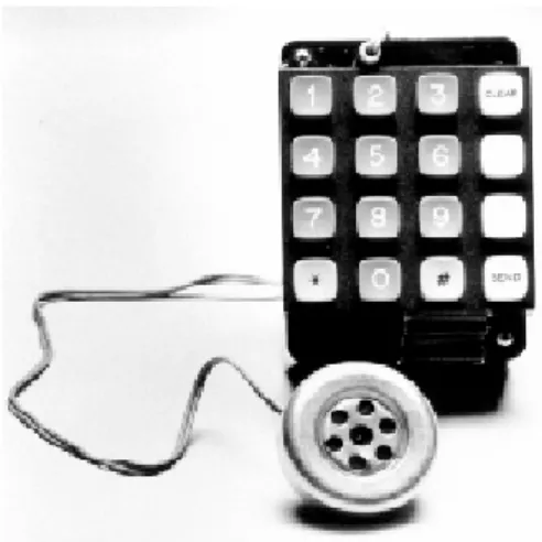
In the 60s The Bell Systems released the paper were the control signal were described [7]. This paper and the previous discoveries made from John Darper and Joe Engressia, allowed for Steve Wozniak and Steve Jobs (yes, the creators of apple) to create a device that allowed the job of phreaking to become much easier. The device was named Blue Box (2.1), and it was a simple box with a keypad and a speaker that would connect to the microphone on the telephone headset. By pressing a key, the device emitted the corresponding sound signal trough the speaker and therefore into the network allowing to access the control with the previous correct frequency whistling effort. The key to MF conversion is visible in table2.1. All these discoveries and the invention of the blue box had a purely academic purpose, but this didn’t discouraged other people to copy the device and abuse its purpose.

More recently, the telecommunications fraud concerns extended to another all new dimension since the commercialization of the internet and to a whole new pack of services. New types of fraud appeared and the operators have less control over the users. This resulted in an increased difficulty in preventing the problem. Carriers keep investing in new security systems in order to prevent and fight the fraudsters, but the fraudsters don’t give up and keep trying to find new ways to bypass those securities. This might results in new types of fraud besides the ones that the security systems could prevent. It is safe to say that there is a everlasting fight between the carriers and the fraudsters. The operators trying to avoid their systems from being attacked and the fraudsters

2.1 Telecommunications Fraud 7

Figure 2.1: Blue Box Device

trying to detect and abuse the weaknesses on the systems [3].

2.1.2 Fraud Methods

Telecommunications is wide area because it is composed by a variety of services like telephones and internet. Fraud in this area is consequently an extensive subject. There are types of frauds that are specific to one service, like the SIM card cloning fraud which is a fraud that can only be committed in the mobile phone service. On the other hand, there are frauds that cover multiple services like subscription fraud, which is associated to the subscription of services, non regarding the type of service. Next, the fraud methods will be described.

• Superimposed Fraud — This kind of fraud happens when the fraudster gains unauthorized access to a client account. In telecommunications, this includes the SIM card cloning fraud that consists in the copy of the information inside the SIM card of the legitimate client to another card in order to use it and access the carrier services. This mean that the fraudster superimposes the client actions pretending to be that person. Despite not being so common lately, it is the fraud who has been most reported in the since its detection. Thus, it has been the object of more studies [8].

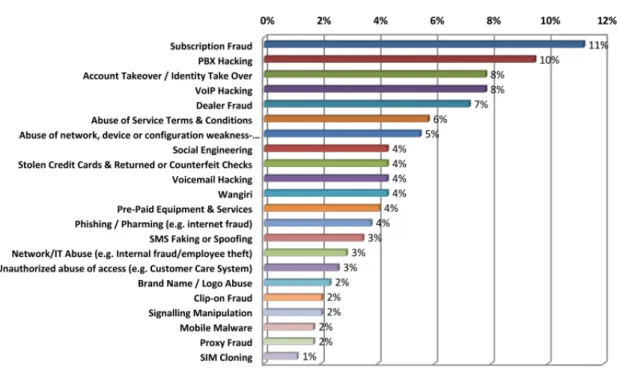
• Subscription Fraud — This fraud occurs when a client subscribes to a service (e.g. inter-net) and uses it without the intention of paying. This is the fraud method that was reported as the most frequent in the year of 2013 (see fig.2.2) [3].

• Technical Fraud — This fraud occurs when a fraudster exploits the technical weaknesses of a telecommunications system for his benefit. These weaknesses are usually discovered by the fraudster in a trial and error methodology or by the direct guidance of an employee who is committing internal fraud. Technical fraud in mostly common on newly deployed services, where the chance of existing an error of development is bigger. Some of these

8 State Of the Art

Figure 2.2: 2013 WorldWide Telecommunications Fraud Methods Statistics.

errors are only fixed after the deployment of the system and in some cases after the fraud being committed. This fraud includes the well known “system hacking” [3].

• Internal Fraud — Happens when an employee of a telecommunications company uses internal information about the system in order to exploit it for personal benefit or the benefit of others. This fraud is usually related with other types of fraud (e.g. technical fraud). • Social Engineering — Instead of trying to discover the weaknesses of a carrier system

(like the trial and error system of technical fraud), the fraudster uses soft skills in order to obtain detailed information about the system. This information can be obtained from the employees of the carrier without them knowing the true intentions of the fraudster. There might even exist a relation between this method and the internal fraud where the fraudster convinces one employee in committing the fraud in his name [3].

Figure2.2displat the fraud methods with more incidences in the year 2013 worldwide.

2.2

Anomaly Detection

Anomaly detection, is one of the areas of the application of data mining which consists in the identification of intances of data which do not fit the pattern defined by the data. An anomaly (or outlier) is the instance of data that do not belong to any pattern predefined as normal or in fact belong to a pattern consider abnormal [9]. In summary, the instances belonging to normal patterns are considered normal and those who don’t belong are considered abnormal. If those patterns are

2.2 Anomaly Detection 9 2 N 1 N 1 o 1 O Y X Figure 2.3: Outliers example in a bidimensional data set.

well defined at an early stage and the model used to do the anomaly detection is well built, this process can also be used in the prediction (prevention) of anomalies. Some example of anomaly detection problems are:

• Fraud detection - telecommunications fraud, credit card fraud or insurances fraud. • Intrusion Detection — network intrusion detection, live house security systems. • Network Diagnoses — network monitoring, network debugging.

• Image Analyses — image processing.

• Failure Detection — networks failure prediction.

The process used to build an anomaly detection model is composed by two stages, the training stage and the test stage. The first stage is the training stage and is used to build the model used for detection. The second stage is the test stage and is used to evaluate the performance of the model [10]. This process usually implies that the available data set is divided in to parts, one for training and the other for testing. These parts usually represent 70% and 30% of the original data set for training and testing respectively.

Anomaly detection wouldn’t be complicated by visual analysis for a small set of data. The problem appears when the amount of data grows exponentially, and the visual analysis starts to be less precise. In figure2.3we can observe two patterns of data in the group N1e N2, one smaller group O1and an instance o1. In the case of anomaly detection, the instance o1 is undoubtedly an outlier and the groups N1 e N2are not outliers. However it can be argued that the smaller group O1can be either a group of outliers or just another group of normal data.

2.2.1 Anomaly Types

When building an anomaly detection system, it is necessary to specify the type of anomaly that the system is able to detect [9]. These anomalies can be of type:

10 State Of the Art

• Point Anomalies — An individual instance that is considered abnormal relative to the rest of the data. This is the most basic type of anomaly. In figure2.3the sample o1is considered a point anomaly. An example of a point anomaly in the telecommunications context is when a client that has a mean call cost of value X and suddenly a call of value Y is made (Y >> X ). Then due to the difference from the mean, the call of cost Y is very likely to be a point anomaly.

• Contextual Anomalies — A data instance that differs from the rest of the data given a certain context (or scenario). The same instance can be classified as normal given a different context. The context definition is defined when formalizing the data mining problem. An example of contextual anomaly in the telecommunications context is when we compare the number of calls made by a user within the business context against personal context. It is more likely for a client to make less calls in the personal context than in the working context. So, if an extraordinary large number of calls appears for that client, it will be considered abnormal in the personal context and normal in the business context.

• Collective Anomalies — A group of related data that is considered anomalous according to the rest of the data set. Individual instances in that group may not be considered anomalies when compared to the rest of the data, but when joined together they are considered an anomaly. An example of collective anomaly in the telecommunications context is when the monitoring system that counts the number of active calls in the infrastructure per second is displaying 0 active calls for a 1 minute period measure. This means that 60 measures were made and all of them were returning 0. A minute without any active calls is very likely to be considered an anomaly, but if we take each one of those 60 measures as a single case, or even smaller groups, then they might be considered normal.

2.2.2 Data Mining

Data mining is a process that allows the extraction of non-explicit knowledge from a data set [11]. It consists in the semi-automatic analysis of the data, attempting to find patterns that summarize the relevant information contained in it. This process is very useful for handling big amounts of data, which is a characteristic of the data generated from the telecommunications companies. A typical data mining problem starts from the need to find extra information from an existing set of data. Each step in the process is measured in order to achieve the maximum amount of information for the planned objective. The steps that compose the standard process are:

• Data cleaning and integration — Cleaning consist in the removal of noise and data that are consider redundant and useless. In the integration phase, data from multiple sources is combined.

2.2 Anomaly Detection 11

• Data Selection and Transformation — In the selection step, only the data that is relevant for the task is selected. This data is prepared for the algorithm used in the data mining pro-cess (next step). Transformation allows the creation of new data derived from the previous data, such as new variables that are a combination of the original ones.

• Data Mining — This is the step where the new knowledge will be extracted from the data. An algorithm is applied to the data in order to obtain a model that represents the data charac-teristics. Some algorithms used in this step are described in the anomaly detection chapter. • Evaluation — In this step the output of the data mining process (previous step) is evaluated.

The performance of the model is measured and the results are evaluated from the point of view of the objective that was initially defined.

• Knowledge Presentation — Presentation of the results to the user. This presentation de-pends of the desire output. It can be a visual presentation like data charts or a tables or it can be another data set that can be used as the input for a new data mining process.

Despite presenting a well-defined order, it doesn’t necessarily mean that to achieve a good result we are only required to execute only once each one of these steps. In most cases a good result only appear after a few iterations of the whole process [12].

2.2.3 Learning Types

When building a model for an anomaly detection process, it is required to know if the data that is being used in the algorithm to construct the model contains examples that are labeled. In other words, if the value of the objective variable is known [9]. The objective variable is the variable that, in the case of anomaly detection data mining, says to which class a given data instance belong to, normal or anomalous. This is also known as the label. The learning type differs regarding the labelling of the input data. The existent learning types are:

• Supervised — The data used to construct the model has labels indicating whether examples are normal or abnormal. This type of learning is very useful for prediction models because it contains information about both classes.

• Semi-Supervised — The data used to construct the model contains both labelled and unla-belled examples. Models using this type of learning usually try to define the launla-belled class properties. Any instances that doesn’t fit in those properties is label in the opposite class. • Unsupervised — The data available is not labelled. One example of this type of learning is

clustering, which groups the examples in the data according to their similarity.

Sometimes the labelling process is made by hand of an analyst. This is a tiring job and due to this, sometimes the amount of labelled data is very tiny. In some cases there might be bad labelling of the data [13].

12 State Of the Art

2.2.4 Model Evaluation

One of the most important steps when building an anomaly detection model, is evaluating its performance. In the case of anomaly detection, this process consists in extracting indicators which allow to compare one model detection output with te original data. The models output can be of two types:

• Labels — for each instance of data, the models outputs a positive or negative label (anoma-lous or normal).

• Scores — for each instance of data the model outputs a value, created by a scoring tech-nique, that represents the degree of anomaly also known as anomaly score. This allows the results to be ranked and give priority anomalies with higher scores. It is also possible to convert an output score into a label by using a threshold.

2.2.4.1 Evaluation Metrics

In anomaly detection, each data instance data can only belong to one of two classes: positive or negative class. The anomolous data is usually represented by the positive class because the objective of the detection process is detect anomolous data. Therefore, the negative class data is the normal data. This notion allows to usage several indicator to evaluate the performance of a given model. Comparing the models output class labels with the original labels 4 indicators can be obtained:

• True Positives (TP) — Amount of positive class instances classified as positive (anomalous instance labelled as anomalous);

• True Negatives (TN) — Amount of negative class instances classified as negative (normal instance labelled as normal);

• False Positives (FP)— Amount of negative class instances classified as positive (normal instance labelled as anomalous);

• False Negatives (FN)— Amount of positive class instances classified as negative (anoma-lous instance labelled as normal);

This allows the calculation of more descriptive measures like the recall and precision, which are the most popular performance indicators for binary classification. Recall is the fraction of the original positive class instances that were classified as positive. Precision is the fraction of predicted positive class instancess that were correctly classified.

precision= T P

T P+ FP (2.1)

recall= T P

2.2 Anomaly Detection 13 0.00 0.25 0.50 0.75 1.00 0.00 0.25 0.50 0.75 1.00

False Positive Rate

T rue P ositiv e Rate Curves: ROC1 ROC2

Figure 2.4: 2 models ROC curve Comparison

2.2.4.2 ROC

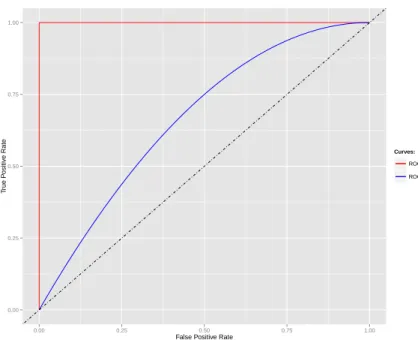
Another interesting approach to describe the model performance is the ROC curve. To plot a ROC curve it is required for the model to output a probability or a ranking of the examples in terms of some scoring function relative to the positive class [12]. This ranking, or probability, describes how likely it is for an instance to belong to the positive class. This curve plots the relation between the True Positive Rate (TPR), or recall, and the False Positive Rate (FPR) when the boundary of decision changes. The boundary of decision is the threshold used to transform the ranking or probability into a class label. The method to draw the curve is then to make the decision boundary to go from the minimum value to the maximum value int the scoring function, and in each step measure the TPR and FPR.

truepositiverate=T P P = T P T P+ FN= recall (2.3) f alsepositiverate=FP N = FP T N+ FP (2.4)

Figure2.4displays the comparison between two ROC curves. Both curves are drawn above the dotted line (X = Y ) which means that the TPR is always bigger than the FPR for every value of the decision boundary. This also means that they are both good models to classify the data. This ROC comparison also displays the perfect model which is represented by the curve ROC1. In the perfect model, all the positive instances have are selected by the model before any negative instance is incorrectly selected.

14 State Of the Art

2.2.4.3 Model Validation

Model validation techniques focus on repeating the model construction and validation stages in different testing and training data and in each experiment, to improve the reliability of the esti-mated values of the performance measures. There are several methods to make the selection of the data used in the train and test stages like the holdout method, k-fold cross-validation, boot-strap and the Monte Carlo experiment. Here, we only describe two of these methods: the k-fold cross-validation and the Monte Carlo experiment.

In the k-fold cross-validation method, the data set is randomly divided into k subsets of the same size with similar initial characteristics (e.g. same class distribution as the original data set). These subsets are also known as folds. At each interaction, nine folds are used for training and, the remaining fold is used for testing. The same fold is never used for training and testing at the same time. The method ends when every fold was used for testing [12]. When k is equal to the size of the data set N, this method is called "leave-one-out" cross-validation.

In the montecarlo experiment, the original data set is partitioned M times into disjoint training and testing subsets. The training and testing data sets are fractions of size ntand nv, respectively, of the original data set. The main feature of this validation method is that, despite the training and testing data sets being randomly generated, they respect the temporal order of the data. Therefore the training data set is generated from randomly selecting data that is on an earlier time interval than the data used for the generation of the testing data set. This method is especially important for validating time series forecasting models [14].

2.3

Data Mining Techniques for Anomaly Detection

In this section, some of the existing techniques that use data mining processes for anomaly detec-tion will be presented.

2.3.1 Clustering based techniques

Clustering is a process that has the objective of partitioning the data into subgroups of instances that have similar characteristics. These groups are called clusters. Anomaly detection using clus-ters is made by applying a clustering algorithm to the data and afterwards, the classification of the data is made by one of the following principles:

• Normal data instances belong to a cluster and abnormal instances don’t — In this case the clustering algorithm shouldn’t force every instance to belong to a cluster.

• Normal data instances are closer to the centroid of the corresponding cluster and ab-normal instances are far from it — The cluster centroid is the graphical centre of the cluster.

• Normal data instances belong to denser clusters and abnormal instances are in less denser clusters — In this case it is requires to measure the density of each cluster of data.

2.3 Data Mining Techniques for Anomaly Detection 15

To define the density value where a cluster belongs to each one of the classes it is required to define a threshold values;

These techniques don’t require the data to be labelled, therefore they are of the type unsu-pervised learning. They also work with several types of data. Although the anomaly detection is fast and simple after the cluster have been achieved, the clustering process may be slow and computational expensive. The performance of the anomaly detection process depends mostly on the clustering process [9].

2.3.2 Nearest neighbour based techniques

Nearest neighbours techniques are based on measures of the distance (or similarity) between data instances. The distance calculation is made by a relation between the attributes of the data in both instances. Anomaly detection approaches based on nearest neighbour can be of two types:

• Kth_{nearest neighbour techniques — This techniques starts by giving each data instance} an anomaly score that is obtained by evaluation of the distance to its kth neighbours. Af-terwards the most usual way to separate anomalous instances from normal instances is by applying a threshold to the anomaly scores calculated previously.

• Relative density techniques — In this technique each instance is evaluated by measuring the density of its neighbourhood. The neighbourhood density is measured by the amount of instances that are within a distance range that is previously defined. It is expected for anomalous data instances to have less dense neighbourhoods and normal data instances to have more dense neighbourhoods.

These techniques can use unsupervised learning, which makes the model construction only guided by the rest of the data features non regarding the class label. In this case, if the normal instances don’t have enough neighbours and the anomalous instances do, the model will fail to correctly label the anomalous instances. Since the key aspect of this technique is the distance function, it allows the adaption of the model to other type of data only requiring to change the way the distance is calculated. This is also the main downside, because bad distances calculation methods will result in poor performance [9].

2.3.3 Statistical Techniques

In statistics techniques the anomaly detection is done by evaluating the statistical probability of a given instance to be anomalous. Therefore the first step in these techniques is the construction of a statistical model, usually for normal behaviour, that fits the given data. The probability of an instance to be anomalous is then derived from the model. In the case that the model represents the probability of normal behaviour, when a data instance is evaluated in the model, the ones that are assigned high probability are considered normal and the ones with low probability are considered anomalous. The probability construction models can be of the type:

16 State Of the Art

• Parametric — Statistical models of this type assume its probabilistic distribution is defined a priori, and parameters which are derived from the given data. An example of a parametric probability distribution is the Gaussian distribution that is defined by parameters of mean (µ) and standard deviation (σ ).

• Non-parametric — These models are entirely based on the data without having a probabil-ity distribution fixed beforehand. An example of model of this type are the histogram based models, in which the histogram is built using the given data.

These techniques outputs scores associated with a confidence interval. The downside of para-metric technique is that works under the assumption that the probabilities are distributed under a specific way which is not true in most cases [9].

2.3.4 Classification Techniques

Anomaly detection using classification techniques requires the construction of a classifier. A classifier is a model constructed under supervised, or semi-supervised, learning algorithm. It represents patterns in the datathat can later be used to classify new data instances as normal or anomalous. There are several classification techniques. The main difference between them are the classifier type (model) that each one builds and use. Some of these approaches are:

• Neural Networks — In this approach during the training stage, a neural network is trained with data from the normal class allowing the model to capture the normal data characteris-tics. Afterwards, data instances are used as input of the network. If the network accepts that instance then it will be classified as normal, if not it will be classified as anomalous. • Bayes networks — In this approach the training stage is used to obtain the prior

probabili-ties for the atributes of the data and class distribution in each class. In the testing stage, the classification is made by calculating the posterior probability (the Bayes theorem) of every class in each data instance. The class with higher probability for that instance, represents the class which that instance is going to be labelled with.

• SVM — In this approach the training stage is used to delimit the region (boundary) where data is classified as normal. In the testing stage, the instances are compared to that region, if they fall in the delimited region they are classified as normal, if not, as anomalous. • Rules – In this approach, the training stage is used to create a group of rules (e.g. if-else

conditions) that characterize the normal behaviour of the data. In the testing stage, every instance is evaluated with those rules, if they pass every condition they are classified as normal, if not, as anomalous.

These techniques use very powerful and flexible algorithms, because it is only required to apply the classifier to each instance. The downside is that supervised learning requires a very ef-fective labelling processs. If any mistakes were made, they will later result in a worse performance

2.4 Data Mining on Fraud Detection 17

of the classifier. The output of this technique is in most of the cases a class label, which his not suitable for scoring [9].

2.3.5 Classification with Unbalanced Datasets

An unbalanced data set is a data set where the number of examples of the existing classes is not balanced. This means that the amount of instances belonging to one of the classes is much more abundant than the other(s). In the case of anomaly detection, it is quite usual for the amount of anomaly instances to be quite smaller than the amount of normal ones. This is a problem because it will make the anomaly detection algorithm to identify easily patterns regarding the normal data but not for the anomalies. A solution to counter this problem is to change the model construction process in order to generate conditions to deal with the unbalanced classes. However this solution is not one of the most common because it requires greater research and changes on the standard model construction algorithm, instead of using off-the-shelf algorithm [15]. Therefore some optional solutions that use off-the-shelf algorithms are:

• Undersample the major class — before constructing the model, remove some instances of the major class (with sampling techniques). This might result in the decrease of information for the undersample class data in the resulting model.

• Oversample the minor class — before constructing the model, repeat some minor class data instances. This will result in some repetitive information being used in the model construction algorithm.

Some additional solutions are based on feature engineering in order to enable the algorithm to find patterns concerning the minority class [16].

2.4

Data Mining on Fraud Detection

Most works on data mining done in telecommunications fraud detection have the objective of de-tecting or preventing the methods of superimposed fraud [8,13] and subscription, [1,17] because these are the fraud types that have done more damage to the telecommunications industry.

2.4.1 Data Format

Projects done in fraud telecommunications aren’t always easy to begin, because companies can’t allow direct access to data of their clients, due to agreements between carrier and the clients. The type of data that is most commonly avaiable to researchers are the CDR, call details records (or call data records)[6,2,1,5,13,17,18]. These records have a log like format and they are created every time the client finishes using a service of the operator. The format of the records may change from company to company but the most common attributes are:

18 State Of the Art

• Date and time;

• Type of Service (Voice Call, SMS, etc...) ; • Duration;

• Network access point identifiers; • Others;

This data doesn’t actually compromise the identification of the users or the content that was traded in the communication, therefore it doesn’t violate any privacy agreement. If some logs do compromise the true identification of the clients, the data can be anonymized by the company before being released.

2.4.2 User Profiling

In most fraud detection studies, the authors choose techniques of user profiling in order to describe the behaviour of the users [19, 6, 5, 2]. User profiling is done by separating the data that has anything to do with a user and develop a model that represent its behaviour. This enables the extraction of additional information from the data used, and even add some additional information to the data set, like new attributes, before doing the model for anomaly detection.

The user models can be optimized by dynamically adapting user profiles [8]. This means that the user model must be updated every time the user makes an interaction with the system. Users don’t have a constant behaviour so the models that define their behaviour should not be static.

Profiling requires a lot of information about the users in order to build the most representative behaviour model. CDRs are very useful to create behaviour models. However to make a more realistic representation of the user, more information is required, which is rather difficult to obtain due to confidentiality agreements.

2.4.3 Rule based applications

T. Fawcett and F. Provost [8], presented a method for superimposed fraud detection based on rules. They used a group of adaptive rules to obtain indicators of fraudulent behaviour from the data. These indicators were used for the construction of monitors. These monitors defined fraudulent behaviour profiles and are used as input for the analysis model, also known as detector [19]. The detectorcombines the output of the monitors with the data generated along the day by a user, and in the case of fraudulent activity, outputs an alarm.

S. Augustin, C. Gaiber, J. Knauer, M. Massoth, K. Piejko, D. Rihm and T. Wiens developed a system for fraud detection in new generation networks[18] . The system is composed by two modules: one for interpretation of data and other for detection of fraud. In the module of interpre-tation, the CDR’s data is used as an input, and the module analyzes and convert that data into CDR objects, which will be used to as input for the classification module. In the classification model,

2.4 Data Mining on Fraud Detection 19

the CDR objects will be subject to a series of filter analysis. The filters are actually rule based classification models that were obtained previously from real fraudulent data. If a CDR object doesn’t respect the rules in those filters an alarm is generated. As a result rate of false-positive 4%.

2.4.4 Neural networks Applications

In the system for fraud detection built by the M. Taniguchi, M, Haft, J, Hollmén and V. Tresp [20], three anomaly detection techniques are used: supervised learning neural networks, parametric statistcal techniques and Bayesian networks. The supervised neural network is used to construct a discriminative function between the fraud and normal classes using only summary statistics. In the parametric statistical technique, the density estimation is generated using a Gaussian mixture model, and it is used to model the past behaviour of every user in order to detect any abnormal change from the past behaviour. The Bayesian networks are used to define the probabilistic models of a particular user and different fraud scenarios, enabling the detection of fraud given a user’s behaviour. In the tests done by the authors, the system had a precision of 100% and a recall of 85%.

2.4.5 Other Applications

The system developed by H. Farvaresh and Mohammad M.Sepehri [17] for subscription fraud was composed by 3 stages: pre-processing, clustering and classification. In the pre-processing stage, the raw data was cleaned, prepared and the transformed using principal components anal-ysis (PCA). In the clustering stage, the data was clustered into homogeneous clusters by the two clustering algorithms SOM and k-means. If the resulting clusters are very specific, very different from other clusters or outlier clusters (one instance cluster), then they are discarded and they are not used in the classification stage. This stage was also used to insert some new features to the data in order to keep the properties of clusters generated previously. In the last stage, the classifi-cation stage, the instances are classified using the classifiers SVM, neural networks and decision trees. The classifitaion is made over different ensembles: bagging, boosting, stacking, voting and standard. The result final result is obtained by the ensemble that offered the best performance.

A very interesting work was done by Kenneth C. Cox, Stephen G. Eick and Graham J. Will [21]. They experimented visual techniques data mining in order to detect anomalies. They claim that these techniques offer one great advantage over learning algorithms, because the systems for the human visualization have better dynamism and adaptability therefore they are better able to cope with the evolution on fraudulent behaviour. These methodology is based in the quality of the graphical presentation of the data on human visual interfaces in order to facilitate the visual fraud detection.

Chapter 3

Naive Bayes

3.1

Algorithm

Naive Bayes is a supervised learning classification algorithm that applies the Bayes’s theorem with an assumption of independence between the data features [22]. This assumption is what make him naive. The Bayes’s theorem in the classification scenario can be described as

P(θ | x1, x2, x3, ..., xn) =

P(θ )P(x1, x2, x3, ..., xn| θ ) P(x1, x2, x3, ..., xn)

(3.1) where x1, x2, x3, ..., xn= X is the data instance (group of features of that instance), θ is the class (positive or negative), P(θ | x1, x2, x3, ..., xn) is the posterior probability or the probability of a given instance X to belong to the class θ , P(θ ) is the prior class probability distribution, P(x1, x2, x3, ..., xn| θ ) is the prior attribute probability given the class θ , and P(x1, x2, x3, ..., xn) is the evidence or instance probability.

The Naive characteristic of this algorithm is visible on the numerator. Before applying the independence property, the numerator can be re-written using the conditional chain rule:

P(θ )P(x1, x2, x3, ..., xn| θ ) = P(θ )P(x1| θ )P(x2, x3, ..., xn| θ , x1)

= P(θ )P(x1| θ )P(x2| θ , x1)P(x3, ..., xn| θ , x1, x2)

(3.2)

After all the features have been separated, the independence between features property can be applied and the equation can be summarized as:

P(θ )P(x1, x2, x3, ..., xn| θ ) = P(θ )P(x1| θ )P(x2| θ )P(x3| θ )...P(xn| θ ) = P(θ ) n

∏

22 Naive Bayes

Prior attribute probabilities are calculated by the following equation:

P(xt | θ ) =

Nt,xt,θ ∑j∈tNt, j,θ

(3.4) where Nt,xt,θ is the amount of instances with attribute t of value xt belonging to class θ [23]. The denominator (P(x1, x2, x3, ..., xn)), is constant in each instance (x1, x2, x3, ..., xn) and results from the sum of the numerator value for all possible classes.

P(x1, x2, x3, ..., xn) = m

∑

∏

Finally, the initial Naive Bayes equation, can be re-written as

P(θ | x1, x2, x3, ..., xn) = P(θ ) ∏n₁P(xi| θ ) m ∑ j=1 {P(θj) n ∏ i=1 P(xi| θj))} (3.6)

3.1.1 Naive Bayes for Classification

If the objective of the Naive Bayes algorithm is to simply classify instances with a label with-out regard for the class probability (or ranking) for each instance, then the classification process doesn’t require the value of the denominator (P(x1, x2, x3, ..., xn)) since it is a constant for each in-stance. The classification process only requires the result of the numerator, P(θ ) ∏n1P(xi| θ ). This characteristic allows the use of Maximum A Posteriori (MAP) value to estimate the values P(θ ) and ∏n1P(xi| θ ) to determine which class θpreddoes a given instance (x1, x2, x3, ..., xn) achieves its maximum value [22]. The resulting classification rule is

θpred= argmaxθP(θ ) n

∏

When constructing the Naive Bayes model, namely calculating the class prior probability (P(θ )), there might be some cases where the data does not offer the necessary information regarding a given feature (xt) for a value (A) in one of the classes (θr), resulting in a prior attribute probability of value zero. This will later result in a posterior probability for an instance with feature xt = A to be zero for the class θr. This results in a model that will never classify an instance with that particular characteristic (xt= A) as belonging to the class θreven if the rest of the features strongly point for that instance to belong θr. To avoid this effect, it is usual to use a method called Laplace Correctionin order to avoid absense of information in the data regarding one of the classes. This method changes the initial value of the count for instances with that characteristic in a given class

3.2 Previous adaptations 23

[24]. The formula for a the prior attribute probability calculation for a given attribute xt on a given class θ is

P(xt | θ ) =

I+ Nt,xt,θ (K ∗ I) + ∑j∈tNt,i,θ

(3.8) where I is the Laplace Correction value (usually 1) and K is the different values that attribute xt can have.

3.1.3 Continuous Variables

Some attributes in the data set might have continues values, this will cause a problem in the likelihood probabilities because it is rather impossible to cover all the values in an interval of continuous values. In order to describe these variables there are some procedures that can be made in order to summarize them. One option is to discretize the variable. In this case the continuous variable will be converted to discrete values (e.g. convert continuous intervals to discrete variables) thus becoming compatible with the standard model construction method. Other common option to describe the continuous variables is by making the assumption that the variable values are follow a parametric probability distribution. This requires some intrinsic adaptions of the Naive Bayes model in order to calculate the likelihood probability using the density distribution function. A popular solution is to use a Gaussian-like distribution. In this case, during training it is only required to calculate the mean (µθ) and standard deviation (σθ) for the feature xt in each class θ [25]. During model construction, the prior atribute probability is given by:

P(xt | θ ) = 1 σθ √ 2πe −(xt−µθ) 2. 2σ_θ2 (3.9)

3.2

Previous adaptations

A previously study presents a correction to the prior attribute probabilities calculation to counter the unbalanced classes effect on the final model [24]. This solution was studied on the application on the Naive Bayes algorithm with objective of text classification. It can actually be applied as a normalization step to the data, enabling the possibility of leaving the Naive Bayes as a off-the-shelf algorithm. In this particular solution, due to the data structure, the prior attribute probability is calculated by the following equation (using the authors notation):

P(w | c) = 1 + ∑d∈Dcnwd k+ ∑w0∑d∈DCnw0d

(3.10) where nwdis the number of times that word w appear on document d, Dcis the collection of all documents belonging to class c and K is the previous explained LaPlace Correction. The objective

24 Naive Bayes

of this author is to normalize the word count in each class in so that the size for each class is the same. To achieve this, the variable nwdis transformed as:

α nwd

∑w0_∑d∈D Cnw0d

(3.11) where α is the normalization constant and defines the amount of smoothing across word counts in the dictionary. When α = 1 the resulting equation is:

P(w | c) =

1 + ∑d∈Dcnwd ∑w0∑d∈DCnw0d

k+ 1 (3.12)

This allows to scale the prior attribute probability in the case of the objective class (or classes) in order boost the posterior probability calculation for word with those characteristics.

3.3

Proposal

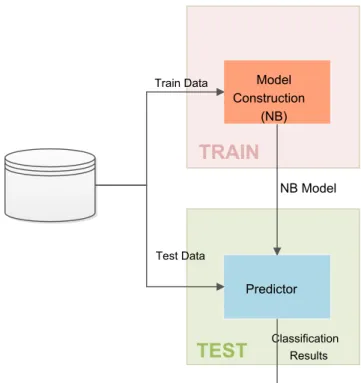
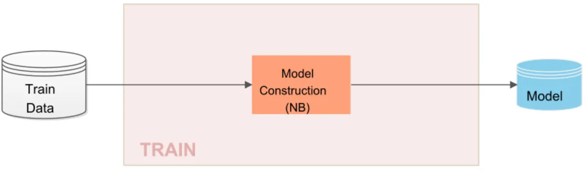
This project proposes the study of two solutions for the anomaly detection system using the Naive Bayes classification algorithm. These proposal are intent to compensate the effect that unbalanced class data generates when constructing the the classification model, and therefore the classification. For comparison purposes, the standard procedure in the classification task is represented in figure3.1

3.3.1 Naive Class Distribution

This solution consists mainly in changing the properties of the model generated by the Naive Bayes algorithm, more precisely the prior class probability ((P(θ ))) of the model. This approach is the result of analysis of the effect of undersampling the data in the major class before constructing the model. Undersampling the data before applying the Naive Bayes algorithm can result in a better class distribution, which affects the prior class probability ((P(θ )))) of the Naive Bayes model. However, it can degrade que information in the prior attribute probability ((P(θ | X ))) of the model, which is the result of removing intances by undersampling data. This process on the other hand is meant to balanced the class probability, and therefore the prior class probability without compromising the prior atribute probability. The assumption made in this solution was: condition the prior class probability without compromising the prior attribute probability, so that the class distribution do not affect the classification. In order to produce this change, the model construction process must have a variable which describes the prior class distribution. In this case the variable used is the Prior Percentage Distribution (PPD). (PPD) is the value to be assigned to the negative class prior probability (P(θN)). Therefore it is also possible to extract the value of the positive class prior probability (P(θP)). The method is specified as:

3.3 Proposal 25 Model Construction (NB) Predictor Classification Results

TRAIN

TEST

Figure 3.1: Standard Naive Bayes model construction squematics

P(θP) = 1 − PPD = 1 − P(θN) (3.14)

An representative illustration of the process is presented on figure3.2.

Comparing to the standard procedure, the main diference is on the training of the model which included Change Prior Probabilities module on the training stage. This module changes the values of the prior class probability (P(θ )) according to the previously set Prior Percentage Distribution value (PPD).

3.3.2 Naive Bayes Margin

This proposal consists on creating additional features to the model generated by the standard al-gorithm. The margin values, mn and mp, are the key aspect of this proposal and they are built upon the following assumption: How can the negative class (major) posterior probability be re-duced and the positive class (minor) posterior probability be increased in order to get more True Positives without compromising the True Negatives. This solution has a similiar characteristics to the method in the SVM classification algorithm, where the margin is the distance to the decision boundary. The procedure, is then to study the posterior probabilities for the True Negatives and False Negativesinstances in the classified train data (classified by the model constructed using

26 Naive Bayes Model Construction (NB) Predictor Classification Results

TRAIN

TEST

Train Data Change

Priori Probabilitie Priori

Percentage Distribution

Figure 3.2: Naive Class Distribution model construction squematics

that same train data) in order to achieve two values that can be applied to the probabilities for both classes in order to obtain better Positive Classification. The process used to generate the margin values (mn and mp) is:

mn=∑i∈TrueNegatives(Pt(θN| i) − 0.5)

T N (3.15)

mp=∑i∈FalseNegatives(Pt(θP| i) − 0.5)

FN (3.16)

where Pt(θN| i) is the posterior probability of instance i to belong to the negative class (θN), T N is the amount of True Negatives, Pt(θP| i) is the posterior probability of instance i to belong to the positive class (θP) and FN is the amount of False Negatives. Note that this process occurs during the training stage, therefore these are posterior probabilities for the train data. Also note that mn, that is the margin value generated from the true negative probabilities, is a positive value while mp, that is the margin value generated from the false negative probabilities, is a negative value.

3.3 Proposal 27

The generated margin values are then applied to the process after the classification process. The application method is represented in the equation:

Pm(θN| X) =    Pp(θN|X)−mn (Pp(θP|i)−mp)+(Pp(θN|X)−mn) (Pp(θN| X) − mn) > 0 0 (Pp(θN| X) − mn) < 0 (3.17) Pm(θP| X) =    Pp(θP|X)−mp (Pp(θP|X)−mp)+(Pp(θN|X)−mn) (Pp(θN| X) − mn) > 0 1 (Pp(θN| X) − mn) < 0 (3.18)

where the Pp(θP, X ) and Pp(θN, X ) are the posterior probabilities generated by classification process with the naive bayes model and Pm(θP, X ) and Pm(θN, X ) are the new posterior probabili-ties after applying the margin to the predictions, both cases for intances X = {x1, x2, ..., xn}. Note that the denominator is only a normalization process that is applied so that posterior probabilities keep the property of Pm(θP, X ) = 1 − Pm(θN, X ).

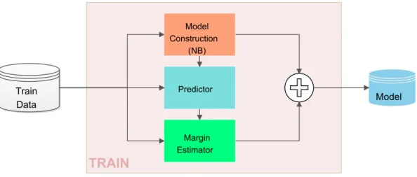
The process for the model construction and the new features generation are represented in figure3.3. Model Construction (NB) Predictor Margin Estimator

Predictor Apply Margin

Classification Results TRAIN TEST Probability Predictions Probability Predictions NB Model Magin Values NB Model Test Data Train Data

Figure 3.3: Naive Bayes Margin model construction squematics

The main differences for this process with the standard procedure are:

• Train — Instead of simply using the training stage to construct the Naive Bayes model, after the construction the resulting model will be used to classify (Predictor in the train area of figure3.3) the same data that is used for its construction (train data). The output of that classification process is in the form of posterior probabilities (Pt(θ | X )). In this case, the

28 Naive Bayes

probabilities for an instance to belong to the positive class (Pt(θP| X)) or the negative class (Pt(θN | X)). Afterwards, the train data and the associated posterior probabilities will feed the margin estimator. The margin estimator is going to derive two new values (mn and mp) from that train data and correspondent classification, that will be used in future predictions. These values are denominated as margin values.

• Test — In the testing stage, the model without the new features is going to be used for the prediction as the typical classification process would do. The output of the prediction process (Pp(θ | X )) also needs to be in the form of class probabilities (like the predictor in the training stage). Instead of using these probabilities to label the test data and finish the process by evaluating the results, the posterior probabilities will feed, together with the pre-vious calculated margin values into the apply margin module. In this module, the posterior probabilities generated by the model (Pp(θ | X )) are re-calculated using the designed algo-rithm and the previously calculated margin values. This process will results in new posterior probabilites (Pm(θ | X )) that will be used to label the data.

Chapter 4

Prediction of Telecom Anomalies

4.1

Data Understanding

The data set used for this project is composed by two days of CDR (Call Details Records) from a telecom company that must remain anonymous for confidentiality reasons. Each data set has the following features (or attributes):

• DATE — date in which the record was created. It is in the format "YYYYMMDD", "YYYY" year, "MM" month and "DD" days. This parameter has only two different val-ues in all examples of the data set used, because there are only two different days.

• TIME — time in which the record was created. It is in the format "hhmmss", "hh" hours, "mm" minutes and "ss" seconds.

• DURATION — is the amount of time, in seconds, that the service lasted. • MSISDN — anonymized cellphone number of user1.

• OTHER_MSISDN — anonymized cellphone number of user2. • CONTRACT_ID — contract indentification number of user1.

• OTHER_CONTRACT_ID — contract indentification number of user2.

• START_CELL_ID — cell identification number for the cell (antenna) where the caller user is accessing.

• END_CELL_ID — cell identification number for the cell (antenna) where the called user is accessing.

• DIRECTION — describes the direction of the call. It can take two values: "I" for inbound and "O" for outbound. This atribute describes the user - Caller/Called. If the value is "I"(inbound) then user1 is the caller and user2 is the called user.

30 Prediction of Telecom Anomalies

• CALL_TYPE — identifier of the type of the call, or service, which the record corresponds to. It can take the following values: "MO", "ON", "FI", "SV" and "OT". A precise descrip-tion of what those values mean was not provided.

• DESTINATION — describes the territorial of the call. It can take two values: "I" for international calls and "L" for local calls.

• VOICEMAIL — a flag-like varialble that takes the value "Y" for calls who went to voice-mail and "N" for calls who are not

• DROPPED_CALL — target variable for the anomaly detection system, or Class. It is a flag-like feature that take two values: "Y" for a dropped call (Positive Class) and "N" for a successful call (Negative Class).

An exploratory data analysis was carried out by computing basic statistics and visualizing the data. Several interesting observations were made, including:

• Cells identifiers, START_CELL_ID and END_CELL_ID, are not available in every in-stance. There isn’t a relation in the call characteristics that justifies the missing value be-cause, in some cases, for calls with the same characteristics there are missing values in both IDs or only one ID or even none of them is missing. This effect could relate to calls which the users are accessing the networks trough cells who don’t belong to the carrier infrastruc-ture, therefore they can’t be identified.

• The contract identifier of user2, OTHER_CONTRACT_ID, in most of the cases is not filled in. This could also relate with the cells identifiers effect explained previously, but in this case it is not the infrastructure that belongs to another carrier but the client.

• All international calls (calls with DESTINATION equal to "I") have the CALL_TYPE feature always equal to "OT", while in the local calls the CALL_TYPE feature can take values of "MO", "ON", "FI" and "SV";

• All calls who went to voicemail (VOICEMAIL have the value "Y") have the CALL_TYPE feature equal to "SV" and all have the same OTHER_MSISDN number. This might corre-spond to the anonymized number of the voicemail center;

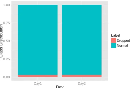
There are some important characteristics about this data that can be displayed through some simple statistics. The total amount of records used for this project is of 14,043,142 for the day1 data set and 13,888,323 for the day2 data set. The class distribution is visibly unbalanced (figure

4.1) where Day1 has about 2.87% dropped calls and Day2 about 2.95%.

There are some important characteristics about this data that are required to be presented be-cause they associate the present data with data that can actually be generated by a true telecommu-nications carrier in a real-world scenario. The first characteristic is presented in figure4.2in which the amount of calls that are made per hour during each of the days are displayed. It is possible

4.1 Data Understanding 31 0.00 0.25 0.50 0.75 1.00 Day1 Day2 Day Class Distr ib ution Label Dropped Normal

Figure 4.1: Class distribution in each day

0 250000 500000 750000 1000000 0 5 10 15 20 Hour Amount of Calls Day Day1 Day2

Figure 4.2: Number of calls per hour in each day

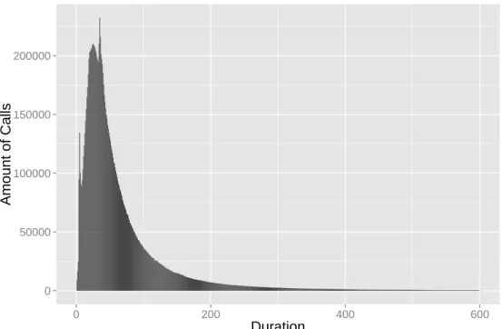
to see that the amount of calls that are done in the day time (8am to 9pm) is much larger than the amount of calls done during the night time (10pm to 7am) which is the expected distribution. Another interesting aspect is shown in figures4.3and4.3. These figures, represent the amount of calls done by duration in each of the two days. In this case, it is possible to observe that most of the calls are of short duration (< 100 seconds) which is very typical on a real-world scenario. The call duration presented in figures4.3and4.4exclude some outlier calls with duration > 5000

sec-32 Prediction of Telecom Anomalies 0 50000 100000 150000 200000 0 200 400 600 Duration Amount of Calls

Figure 4.3: Number of calls by duration in day 1

0 50000 100000 150000 200000 0 200 400 600 Duration Amount of Calls

Figure 4.4: Number of calls by duration in day 2

onds. One important property that can be obtained from this figures that is going to help the model construction is that, the call duration presents a Gaussian-like distribution (see section3.1.3).