Performance evaluation of European SRI fixed-income funds

Rui Miguel Almeida Moreira

Performance Evaluation of European SRI

fixed-income funds

Masters Dissertation

Master in Finance

Work done under the guidance of:

Professor Nelson Areal

DIREITOS DE AUTOR E CONDIÇÕES DE UTILIZAÇÃO DO TRABALHO POR TERCEIROS Este é um trabalho académico que pode ser utilizado por terceiros desde que respeitadas as regras e boas práticas internacionalmente aceites, no que concerne aos direitos de autor e direitos conexos.

Assim, o presente trabalho pode ser utilizado nos termos previstos na licença abaixo indicada. Caso o utilizador necessite de permissão para poder fazer um uso do trabalho em condições não previstas no licenciamento indicado, deverá contactar o autor, através do RepositóriUM da Universidade do Minho.

Atribuição-NãoComercial-SemDerivações CC BY-NC-ND

Acknowledgements

I would first like to thank my dissertation supervisor, Professor Nelson Areal, who persistently provided me his guidance, knowledge, availability and patience. Also to my master colleagues and friends who throughout this entire demanding journey of researching and writing a

dissertation motivated and helped me to overcome all the obstacles that appeared. Finally, I want to thank my family for providing me unfailing support since the beginning to end of my academic years. This accomplishment would not have been possible without them.

STATEMENT OF INTEGRITY

I hereby declare having conducted this academic work with integrity. I confirm that I have not used plagiarism or any form of undue use of information or falsification of results along the process leading to its elaboration.

I further declare that I have fully acknowledged the Code of Ethical Conduct of the University of Minho.

Performance Evaluation of European SRI fixed-income funds

Abstract

In recent years, the investment in SRI securities is experiencing an increasing growth which has attracted a lot of interest from academics and practitioners on their financial performance. Surprisingly the empirical evidence focuses more on the SRI equity market, leaving the SRI fixed-income market less explored. Therefore, in this dissertation, I will try to fill this gap by evaluating the performance of 395 European SRI fixed-income funds during the period of December 1998 to October 2018. The multi-factor unconditional and conditional models were used as performance measures. Results show that the conditional models lead to higher explanatory power of the models, which goes in agreement with the empirical evidence. When considering the performance estimates, the conditional models indicate a slight worst performance, which is controversial with previous studies, although for both the unconditional and conditional model the main conclusion is that the SRI bond funds used on this dissertation underperform the market. Keywords: fixed-income funds; fund performance evaluation; socially responsible investment; unconditional and conditional model

Avaliação do Desempenho de fundos Europeus de obrigações

socialmente responsáveis

Resumo

Nos últimos anos, o investimento em títulos financeiros socialmente responsáveis está a experienciar um crescimento exponencial e consequentemente está a haver um grande interesse dos académicos e investidores no seu desempenho financeiro. Surpreendentemente as evidências empíricas focam-se no mercado de ações socialmente responsáveis, deixando o mercado de obrigações socialmente responsáveis pouco explorado. Assim sendo, nesta dissertação, vou tentar preencher esta lacuna ao avaliar o desempenho de 395 fundos de obrigações europeias socialmente responsáveis durante o periodo de Dezembro de 1998 até Outubro de 2018. Os modelos incondicionais e condicionais multifatoriais foram usados como medidas de desempenho. Os resultados mostram que o modelo condicional leva a um maior poder explicativo dos modelos, o que vai de acordo com a evidência empírica. Ao considerar as estimativas de desempenho, o modelo condicional indica um desempenho ligeiramente pior, o que é controverso com os estudos anteriores, apesar de para ambos os modelos a principal conclusão a retirar é que os fundos de obrigações socialmente responsáveis usados nesta dissertação apresentam uma performance pior que o mercado.

Palavras-chave: avaliação do desempenho de fundos; fundos de obrigações; investimentos socialmente responsáveis; modelo incondicional e condicional

Table of Contents

1.

Introduction ... 1

2.

Literature Review ... 3

3.

Methodology ... 6

4.

Data ... 8

4.2. Returns and Factors ... 9

4.3. Public Information Variables ... 9

5.

Empirical Results... 11

6.

Conclusions ... 21

7.

Appendixes ... 23

8.

References ... 36

1. Introduction

Socially responsible investment (SRI) is not a new type of investment since its roots date back to the money management practices of the Methodists, more than 200 years ago, and empirical analyses of SRI funds dates back to the pioneer study of Moskowitz (1972). Although not being new in the financial market, in recent years a growing concern about climate change and its risks for SRI portfolios is intensifying the interest in this subject. It is notable the number of studies produced by the academic community on SRI fund performance. SRI funds differ from conventional funds by applying not only financial but also moral, social and environmental criteria when making investment decisions. Furthermore, according to Climent and Soriano (2016) one can classify SRI funds in to a more specific group according to the criteria used in their composition (financial, environmental, social and/or ethical criteria).

Over the last years socially conscious investing is becoming a widely followed practice, as the largest institutional investors around the world are acknowledging that investing based on SRI principles is a viable approach of meeting not only their financial objectives but also their social duties (Derwall and Koedijk, 2009).

Empirical studies mainly focus on SRI common stock funds, whereas the performance of SRI fixed-income funds has received far less attention which is limiting strategic and tactical asset allocation decisions (Leite and Cortez, 2018). Therefore, it is important to develop studies on SRI bond funds creating more detailed historical financial record, in order to make optimal strategic and tactical asset allocation decisions. Furthermore, almost every study was conducted in the US (which is by far the most developed market for SRI) and in the UK, leaving the rest of Europe with little research and understanding on the performance of SRI funds (Areal et al. 2009).

There are a number of alternative theories about whether incorporating social screens into investment portfolios affects the financial performance. Following Modern Portfolio theory (Markowitz, 1952) which states that risk is an investment’s characteristic inherently linked to the expected return, socially screened portfolios will create an obstacle for diversification which will

criteria overlooks the financial advantages that environmental, social and governance (ESG) criteria provides. ESG criteria stands to the three main factors that investors consider when regarding a firm’ sustainable practices and ethical impact.

The first social screening strategy used in the investment decision procedure was negative screening which aims to avoid companies involved in sectors such as tobacco, alcohol, armaments or gambling. During the 1990s funds began to incorporate positive screening into the investment process and according to Derwall and Koedijk (2009) nowadays most of US and UK SRI funds use a combination of negative and positive screens. Positive screenings targets companies who promote social and/or environmental sustainability practices. In recent years the positive/best-in-class screening process is becoming widely used when creating funds’ portfolios (Derwall and Koedijk, 2009). “Best-in-class” screening is a process that rather than excluding sectors uses a positive screening within each sector and selects the companies or projects with better ESG performance within each sector.

The market for sovereign government debt is very large and it’s becoming a new propitious market for investors who want to invest according to social and ethical criteria. In this context of investment, the “best-in-class” screening process is the one to use due to the fact that the SRI approach is more focused on sustainability and environmental criteria.

The objective of this dissertation is to evaluate the performance of European SRI fixed-income funds by the means of unconditional and conditional multi-factor models in order to analyze if investing in SRI bond funds brings profitability, represents a financial sacrifice or provides a neutral performance. I chose this theme due to the fact that, to the best of my knowledge, there is only one study that focuses on the performance evaluation of European SRI fixed-income funds using the conditional multi-factor model that allows time-varying risk (betas) and time-varying estimates of performance (alphas). Therefore, in order to gather more empirical evidence on whether this type of investment is a good asset allocation decision or not, I will follow the pioneer study of Leite and Cortez (2018) on the evaluation of European SRI Bond funds using the conditional multi-factor model.

2. Literature Review

As it was previously said most of the SRI mutual funds empirical studies focus on the US equity market and the UK equity market. As far as I am aware there are very few studies on the performance of SRI bond funds. Some authors I found useful for my dissertation are the following: Blake et al. (1993) Elton et al. (1995), Aragon and Ferson (2006) and Hoepner and Nilsson (2017) whose studies concentrate on US bond funds; Silva et al. (2003) whose study focuses on European bond funds and Ayadi and Kryzanowski (2011) that analyzes Canadian fixed-income funds. However the studies I will concentrate on when developing my dissertation are the studies of Goldreyer and Diltz (1999); Derwall and Koedijk (2009); Henke (2016) and Leite and Cortez (2018) since these were the only studies, to the best of my knowledge, that evaluate the performance of SRI bond funds.

Blake et al. (1993) and Elton et al. (1995), studies’ samples consist of US bond mutual funds. To evaluate the financial performance they used traditional measures of performance (single-index model, multi-index model and APT models) and their results show that the average performance after costs is negative. Also their results indicate that the single-index model overestimates the funds’ performance in comparison to the multi-index model.

Aragon and Ferson (2006) using conditional performance evaluation techniques, evaluate the performance of US bond mutual funds and results show that is typical to have an underperformance after expenses.

The studies of Blake et al. (1993), Elton et al. (1995) and Aragon and Ferson (2006) have very similar samples. Although Blake et al. (1993) and Elton et al. (1995) use traditional models and Aragon and Ferson (2006) use the modern conditional model, the financial performance results are the same.

Silva et al. (2003) evaluate the performance of a sample that includes 638 European bond funds from Italy (58), France (266), Germany (90), Spain (157), UK (45) and Portugal (22) using unconditional and conditional models on two sub-periods, February 1994 to December 1997 and January 1998 to December 2000. Also they decided to compare the performance evaluation of a

suggest that the funds under analysis underperform passive strategies and that adding more factors has a greater impact than adding public information variables.

Ayadi and Kryzanowski (2011) constructed two samples of Canadian fixed-income funds. The first sample has 209 fixed-income active funds; the second sample consists of 94 fixed-income dead funds and for both samples the time period is 1984-2003. Using the unconditional single- and multi-factor model and the conditional single- and multi-factor model the results show an underperformance using net returns and an outperformance using gross returns.

Both the studies of Silva et al. (2003) and Ayadi and Kryzanowski (2011) follow the research of Ilmanen (1995) when selecting the appropriate public information variables to estimate their conditional models.

Hoepner and Nilsson (2017) study’ sample consists of 5240 bonds from 425 US companies during the period of January 2001 to December 2014. An extension of the four factor model of Elton et al. (1995) is used to evaluate the performance of the funds when screened with ESG criteria. The results show that investors see ESG fixed income portfolios as riskier and therefore tend to stay away from this type of investment.

Goldreyer and Diltz (1999) conduct a research on the performance of 9 bond and 11 balanced US SRI funds. The results show that the average alpha (Jensen, 1968) of SRI funds was negative, during the period of 1981-1997, whereas conventional funds had positive alphas suggesting that SRI bond funds in the US underperform their conventional peers. In this study the performance evaluation was conducted using a single-index model, and as it is well known the single-index measure has limitations so these results have to be taken with caution.

Derwall and Koedijk (2009) concentrates on 15 bond funds and 9 balanced funds compared to matched samples of conventional funds over the period of 1987-2003. Following the four-factor model developed by Elton et al. (1995), alternative unconditional multi-four-factor model specifications are used to evaluate the funds’ performance. The results show that there are no significant differences of performance between SRI bond funds and their matched conventional peers but SRI balanced funds outperformed balanced funds by 1,3%.

Henke (2016) follows the study of Derwall and Koedijk (2009) and uses a larger sample of 103 SRI bond funds (65 in Eurozone and 38 in US) from the period of 2001-2014 in comparison

to characteristics-matched conventional funds. To evaluate the performance of these SRI funds an unconditional five-factor model, based on Elton et al. (1995), is used. The results suggest that SRI bond funds outperform conventional funds both in the Eurozone and the US and with a portfolio holdings evaluation, it is shown that this outperformance is generated by the ESG screening of the SRI bond funds by having fund managers excluding SRI bonds with poor CSR activities. This strategy is called “worst-in-class” exclusion and it’s unique to SRI bond investments. Furthermore, this study suggests that this approach is more successful during crisis periods (where abnormal returns of socially screened bond portfolios occur) rather than non-crisis periods.

One big limitation of Derwall and Koedijk (2009) and Henke (2016) studies is that conditional models that allow for time-varying alphas and betas were not used. It is known that conditional models that provide time-varying risk and performance are considered more robust models regarding the performance evaluation of funds.

Leite and Cortez (2018) focuses on 51 SRI funds (28 SRI bond funds and 23 SRI balanced funds) and 153 matched samples of conventional funds (84 bond funds and 69 balanced funds) over the period of 2002-2014. In terms of SRI funds, 37 are domiciled in France and 14 in Germany. The main model is the four-factor model of Elton et al. (1995) and Derwall and Koedijk (2009) and they extend it by adding the GIIPS factor to account for the European sovereign debt crisis that emerged in 2008. They use conditional multi-factor models that allow for time-varying risk and performance to evaluate the funds’ performance and to choose their public information variables they follow the studies of Ilmanen (1995), Silva et al. (2003) and Ayadi and Kryzanowski, (2011). The authors show that SRI balanced funds perform similarly to conventional funds, whereas SRI bond funds significantly outperform their peers. The SRI bond funds dataset were divided into corporate bond funds and diversified bond funds (funds investing also in government bonds). The results showed that only bonds funds that included government investing outperformed conventional funds.

3. Methodology

The empirical findings suggest that conditional models are widely recognized as theoretically more robust than the unconditional ones because unconditional measures can provide biased results (Aragon and Ferson, 2006; Jagannathan and Wang, 1996).

The first analysis will be made by the use of the unconditional model, the traditional measure of fund performance. The unconditional model doesn’t consider time-varying risk (constant risk) imputing abnormal performance to fund evaluation (see Breen, Glosten and Jagannathan (1989) for an example). This analysis will give me the opportunity to compare my results with the results of the previews studies.

The conditional multi-factor model (partial version), developed by Ferson and Schadt in 1996, accounts for risk exposure to vary over time (betas) according to market conditions. Christopherson et al. (1998) extended this conditional model (full version) to allow not only time-varying risk (betas) but also time-time-varying estimates of performance (alphas) depending on public information variables available to investors at the time the returns were generated.

Therefore, due to the fact that unconditional models can result in biased estimates of performance, in a second analysis I will use the extended version of the conditional multi-factor model, developed by Christopherson et al. (1998) to evaluate the performance of my SRI funds dataset.

The main model that will be used is a four-factor model developed by Elton et al. (1995) used in the studies of Derwall and Koediijk (2009), Henke (2016) and Leite and Cortez (2018). This model includes a bond market index, a default spread, an option variable and a stock market index. The first factor, the bond market index, tries to capture the influence of different investment-grade bonds in my portfolios. The second factor, the default spread, aims to capture default risk compensation in bond portfolio returns. The third factor, the option factor, is the return difference between a mortgage-backed securities index and a bond market index and its inclusion accounts for the option features of different bonds. Finally, the equity factor is the excess return of a stock market index and its inclusion is relevant because bond funds may hold convertible debt. Also due to the financial crisis that appeared in 2008 in the European sovereign debt market, my research will follow Leite and Armada (2017) and Leite and Cortez (2018) and include an additional factor (GIIPS) which relates to the countries more affected by this financial

crisis. This factor will provide information on the difference in the sovereign bond returns from GIIPS and the other original Euro-area countries.

𝐑𝐩,𝐭− 𝐑𝐟,𝐭= 𝛂𝟎𝐩+ 𝛃𝟏𝐩𝐁𝐨𝐧𝐝𝐈𝐧𝐝𝐞𝐱𝐭+ 𝛃𝟐𝐩𝐃𝐞𝐟𝐚𝐮𝐥𝐭𝐭+ 𝛃𝟑𝐩𝐎𝐩𝐭𝐢𝐨𝐧𝐭+ 𝛃𝟒𝐩𝐄𝐪𝐮𝐢𝐭𝐲𝐭+ 𝛃𝟓𝐩𝐆𝐈𝐈𝐏𝐒𝐭+ 𝛆𝐩,𝐭 (1)

Where Rp,t - Rf,t represents the excess returns of portfolio p over period t; BondIndext the excess

return of a bond index; Defaultt is the return spread between a high-yield bond index and a

sovereign bond index; Optiont is the return difference between a mortgage-backed securities index

and a bond sovereign index; Equityt is the excess return of a stock market index; GIIPSt is the

difference between the sovereign bond returns from GIIPS and the other original Euro-area countries and ԑp,t is a residual term. A statistically significant positive alpha indicates

outperformance, whereas significantly negative alphas show underperformance.

The first model is an unconditional model because it assumes the performance and the risk to be constant. Therefore in this final model it’s important to incorporate conditioning information to transform the previous multi-factor unconditional model into the full version of the conditional model developed by Christopherson et al. (1998) where it will be possible to have time-varying alphas and betas. In this final model, alphas and betas are specified as linear functions of a vector, Zt-1. According to the pioneer authors, Ferson and Schadt (1996) and Christopherson et al.

(1998), Zt-1 represents the public information available for managers in period t-1 that is relevant

for predicting returns in period t.

𝐑𝐩,𝐭− 𝐑𝐟,𝐭= 𝛂𝟎𝐩+ 𝐀′𝟎𝐩𝔃𝐭−𝟏+ 𝛃𝟏𝐩𝐁𝐨𝐧𝐝𝐈𝐧𝐝𝐞𝐱𝐭+ 𝛃′_𝟏𝐩(𝔃𝐭−𝟏𝐁𝐨𝐧𝐝𝐈𝐧𝐝𝐞𝐱𝐭) + 𝛃𝟐𝐩𝐃𝐞𝐟𝐚𝐮𝐥𝐭𝐭

+ 𝛃′

𝟐𝐩(𝔃𝐭−𝟏𝐃𝐞𝐟𝐚𝐮𝐥𝐭𝐭) + 𝛃𝟑𝐩𝐎𝐩𝐭𝐢𝐨𝐧𝐭+ 𝛃′𝟑𝐩(𝔃𝐭−𝟏𝐎𝐩𝐭𝐢𝐨𝐧𝐭) + 𝛃𝟒𝐩𝐄𝐪𝐮𝐢𝐭𝐲𝐭 (2)

+ 𝛃′

𝟒𝐩(𝔃𝐭−𝟏𝐄𝐪𝐮𝐢𝐭𝐲𝐭) + 𝛃𝟓𝐩𝐆𝐈𝐈𝐏𝐒𝐭+ 𝛃′𝟓𝐩(𝔃𝐭−𝟏𝐆𝐈𝐈𝐏𝐒𝐭) + 𝛆𝐩,𝐭

Where 𝓏t-1 is a vector of the deviations of Zt-1 from the average values; β1p, β2p, β3p, β4p and β5p are

average betas; β’1p, β’2p, β’3p, β’4p andβ’5p are vectors that capture the sensitivity of the conditional

betas to the information variables, A’0p is a vector that measures the sensitivity of the conditional

4. Data

4.1. Dataset

This section describes the dataset used throughout this study. During the first week of November 2018, by accessing the platform http://yourSRI.com (the leading database and research engine for ESG and Carbon reporting, monitoring and controlling) 399 SRI fixed-income funds from Europe were selected. One important limitation of this website and therefore of this dissertation is that all the funds considered in there are active funds so it must be taken to account that the dataset of this study only consists on active SRI funds. After selecting the funds I would base my work on the next step was to collect all this data from DataStream, available at the school of Economics and Management at the University of Minho. Through the International Securities Identification Numbers (ISIN) I collected all the available data and ended up with a final dataset of 395 SRI fixed-income funds. In addition to this criterion all of my dataset have at least 24 observations throughout the time period considered and have an investment policy focused on Euro-denominated bonds. It’s important to notice that since the benchmarks I used only have recorded data since December 1998, the time period considered in this study is from 31/12/1998 to 31/10/2018. Also it’s important to acknowledge that, since this data was collected in the first days of November of 2018 I can assume that these funds are considered SRI funds at this date which doesn’t mean that in the past they were already SRI. Due to the purpose of my dissertation I will assume that all the funds are SRI funds throughout the time period considered.

In order to have more robust results I created several portfolios. The first portfolio of this study is the ‘Overall Portfolio’ where all of my dataset is represented. The second portfolio I created is the ‘Lipper Category Portfolio’ where according to the ‘Lipper Global Classification’ variable my dataset was divided into four different sub-portfolios: Convertible, Corporate, Government and Other bonds. To the ‘Overall Portfolio’ and each category of the ‘Lipper Category Portfolios’ I applied a regression analysis and their empirical results will be discussed in the next section.

For each of my five portfolios I applied an unconditional model and a conditional model, discussed in the previous section, and made a comparison between these two types of models.

4.2. Returns and Factors

Using DataStream the fund’s end of the month total return indices were collected. To treat this data, discrete returns for each fund and an ‘Equally Weighted Portfolio’ for each of the five portfolios of this dissertation were calculated.

Either when applying the unconditional or conditional model the benchmarks for each one of the five factors are the same in the five portfolios with the exception of the bond factor. For the ‘Overall Portfolio’, the ‘Lipper Category Convertible Portfolio’ and the ‘Lipper Category Other Portfolio’ the benchmark used in the bond factor was the Iboxx Euro Overall. For the ‘LC Corporate Portfolio’ the benchmark used in the bond factor was the ICE BofA ML Euro Corporate and for the ‘LC Government Portfolio’ the benchmark used was the Iboxx Euro Sovereigns. Each of these bonds factors excess returns were calculated using the 1 month Euribor.

The default spread factor was estimated as the return difference between the ICE BofA ML Euro High Yield Index and the Iboxx Euro Sovereigns. The option factor was estimated as the return difference between the ICE BofA ML Euro ABS and MBS and the Iboxx Euro Sovereigns. To compute the equity factor, excess returns of the FTSEurofirst 300 were calculated using the 1 month Euribor. Finally, to proxy the GIIPS, the difference between the averages returns of the Iboxx Euro Sovereign indices for GIIPS (Greece, Italy, Ireland, Portugal and Spain) and the Iboxx Euro Sovereign indices for the other original Euro-area countries (Austria, Belgium, Finland, France, Germany, Luxembourg and the Netherlands) were calculated.

4.3. Public Information Variables

Regarding the conditional model I decided to use the three standard public information variables (1-month lagged) that several studies (Ilmanen, 1995; Silva et al., 2003; Ayadi and Kryzanowski, 2011; Leite and Cortez, 2018) found useful as predictors of bond returns: a term spread, a real bond yield and an inverse relative wealth. The first two variables are alternative proxies for the overall expected bond risk premium and the last variable is a proxy for time-varying risk aversion.

Government Index) and the year-on-year European Union inflation rate. The inverse relative wealth variable (IRW) is measured as the ‘exponentially weighted average of past real wealth to current real wealth’ of the FTSE Eurofirst 300 index deflated by the European Union Consumer Price - Harmonized Index (HICP), as follows:

𝐈𝐑𝐖𝐭= 𝐞𝐰𝐚𝐖_𝐭−𝟏

𝐖𝐭 = (𝐖𝐭−𝟏+ 𝐜𝐨𝐞𝐟 ∗ 𝐖𝐭−𝟐+ 𝐜𝐨𝐞𝐟

𝟐_{∗ 𝐖}

𝐭−𝟑+ ⋯ ) ∗ (𝟏 − 𝐜𝐨𝐞𝐟)/𝐖𝐭 (3)

Where ewaWt-1 is the exponentially weighted average of the real wealth level until period t-1, Wt

is the level of real wealth in period t and coef represents the smoothing coefficient. Following Ilmanen (1995), Silva et al. (2003) Ayadi and Kryzanowski (2011), and Leite and Cortez (2018), I applied a smoothing parameter of 0.90 and a 36-month window.

With the objective of avoiding spurious regressions biases that arise because these variables tend to be persistent regressors, I followed the procedure suggested by Ferson, Sarkissian and Simin (2003) and stochastically detrended these series by subtracting a 12-month trailing moving average. Finally, in order to have a simple interpretation of the estimated coefficients, these variables were used in their zero mean form as in Ferson and Schadt (1996), Cortez, Silva and Areal (2009), Ayadi and Kryzanowski (2011) and Leite and Cortez (2018).

5. Empirical Results

5.1. Unconditional Model

The first analysis of this dissertation consists on applying the unconditional model for each of the existing portfolios.

Before estimating the regressions analysis of the portfolios I checked the correlation matrix of the independent variables, for each one. Regarding the correlation matrix, the variables should not correlate too highly (multicollinearity). As it can be seen at the tables 6, 7 and 8 in the Appendix,no problems were found on the correlation between the variables of each portfolio.

If multicollinearity occurs it is difficult or impossible to determine the unique contribution of the independent variables. To test for multicollinearity, in every regression model, for each portfolio I estimated the ‘Variance Inflation Factor’ for each variable. As stated by Marquaridt (1970, p.610) “A rule of thumb for choosing the amount of bias to allow with ill conditioned data whether by ridge or generalized inverse, is that the maximum variance inflation factor usually should be larger than 1.0 but certainly not as large as 10”, therefore, by looking at the tables 9, 10, 11, 12 and 13 in the Appendix, since all the values are below 10 and over 1, I can assume that multicollinearity is not a problem in my regression models.

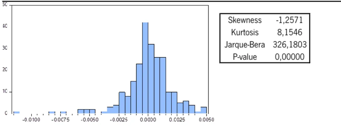
To test the normality of the regression residuals I checked their respective skewness, kurtosis and Jarque-Bera test. When the returns are normally distributed they have a skewness of 0 and a kurtosis of 3. The Histograms and the Jarque-Bera normality tests of the regression residuals are presented in the Figures 1, 2, 3, 4 and 5 in the Appendix. For every portfolio, the results show a skewness different from 0 and a kurtosis different from 3 and the Jarque-Bera results indicate that I can reject the null hypothesis of skewness being 0 and the kurtosis being 3. Therefore, the returns of these regressions are not normally distributed and the statistical test results must be interpreted with caution.

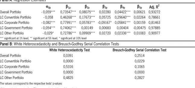
Table 1 presents in Panel A the regression estimates of all the portfolios of this dissertation using the unconditional model and in Panel B the respective White’s Heteroscedasticity and

the β1, β2, β3, β4 and β5 stand for the unconditional betas of the bond factor, default factor, option

factor, equity factor and GIIPS factor, respectively. In Panel B the White (1980) heteroscedasticity test is used since all portfolios don’t present a normal distribution and the Breusch-Godfrey Serial Correlation test. Standard errors are corrected, when suitable, for the presence of heteroscedasticity using the correction method of White (1980), or for the presence of heteroscedasticity and serial correlation using the correction procedure of Newey and West (1994).

Analyzing Panel A, I can see that, for all the portfolios, the lowest adjusted R2 is 78,6% (LC

Convertible Portfolio) and the highest is 97,8% (LC Government Portfolio) which indicates that the five-factor model does a very good job explaining the returns of each portfolio.

At a 5% level of significance, only the ‘LC Convertible Portfolio’ and the ‘LC Other Portfolio’ don’t provide statistically significant alphas. The alphas of the others 3 portfolios display very similar negative alphas which indicate an underperformance.

TABLE 1. Regression Estimates, Heteroscedasticity and Serial Correlation tests using the unconditional 5-factor model

Panel A: Regression Estimates

α0p β1p β2p β3p β4p β5p Adj. R2 Overall Portfolio - 0,059*** 0,73547*** 0,08075*** 0,02280 0,04422*** 0,00621 0,93272 LC Convertible Portfolio - 0,058 0,46268*** 0,17673*** 0,05725 0,29640*** 0,02264 0,78661 LC Corporate Portfolio - 0,082*** 0,77991*** 0,05783*** -0,09167* 0,05841*** 0,00159 0,81463 LC Government Portfolio - 0,054*** 0,74062*** 0,00149 0,00683 0,00404 -0,00475 0,97885 LC Other Portfolio - 0,029* 0,72786*** 0,09909*** 0,02720 0,02336*** 0,01083 0,90977

*** significant at 1% level, ** significant at 5% level, * significant at 10% level

Panel B: White Heteroscedasticity and Breusch-Godfrey Serial Correlation Tests

White Heteroscedasticity Test Breusch-Godfrey Serial Correlation Test

Overall Portfolio 0,0391 0,2514

LC Convertible Portfolio 0,0000 0,0229

LC Corporate Portfolio 0,5316 0,1065

LC Government Portfolio 0,0000 0,0000

LC Other Portfolio 0,4825 0,2827

The values correspond to the respective tests' p-values

If the p-value is greater than 5% we cannot reject the null hypothesis

Panel A presents the regression estimates using the unconditional 5-factor model for five equally weighted portfolios of SRI bond funds, created according to the variable 'Lipper Global Classification'. The time period of this analysis is from December 1998 to October 2018. The unconditional alpha (α) expressed in percentage, the systematic risk of the different factors (β), the levels of significance of each coefficient (by asterisks) and the adjusted coefficient of determination (adj. R2_{) are presented.}

In the five portfolios the benchmarks for each one of the five factors are the same with the exception of the bond factor. The bond factor is represented has β1and

indicates the monthly excess returns of the Iboxx Euro Overall benchmark for the ‘Overall Portfolio’, the ‘LC Convertible Portfolio’ and the ‘LC Other Portfolio’; of the ICE BofA ML Euro Corporate benchmark for the ‘LC Corporate Portfolio’ and of the Iboxx Euro Sovereigns benchmark for the ‘LC Government Portfolio’. Excess returns were calculated using the 1month Euribor as the risk free rate. The default factor is represented by β2and is estimated as the return difference between the ICE BofA ML Euro

High Yield Index and the Iboxx Euro Sovereigns. The option factor is represented by β3and is computed as the return difference between the ICE BofA ML ABS & MBS

Index and the Iboxx Euro Sovereigns. The equity factor is represented by β4and indicates the monthly excess returns of the FTSEurofirst 300 with the 1month Euribor as

the risk free rate. The GIIPS factor is represented by β5and is computed as the difference between the averages returns of the Iboxx Euro Sovereign Indices for the GIIPS

countries and the other original Euro-area countries. Panel B presents the White (1980) Heteroscedascity test since all portfolios don’t present a normal distribution and the Breusch-Godfrey Serial Correlation test. Standard errors are corrected, when suitable, for the presence of heteroscedasticity using the correction method of White (1980), or for the presence of heteroscedasticity and serial correlation using the correction procedure of Newey and West (1994).

Interpreting the benchmarks coefficients, at a 5% level of significance, for the ‘Overall Portfolio’, ‘LC Convertible Portfolio’, ‘LC Corporate Portfolio’ and the ‘LC Other Portfolio’ all the betas are statistically significant with the exception of the option factor and the GIIPS factor. For the ‘LC Government Portfolio’ only the bond market factor is significant. Therefore, I can assume that the option factor and GIIPS factor are not relevant for my analysis, meaning that my funds don’t exhibit option features (mortgage-backed securities) and the financial crisis of 2008 didn’t affect the performance of these European SRI bond funds. For all the portfolios, the factor with the highest exposure is the bond market factor due to the fact of being a benchmark that captures the returns variances of a market with similar characteristics for each portfolio. For all the portfolios apart from the ‘LC Convertible Portfolio’, the default factor shows a significant lower exposure which illustrates low default risk compensation. The equity factor, for all the portfolios with the exception of the ‘LC Convertible Portfolio’, is significant but has a residual load since it is a benchmark that captures the excess returns of a stock market and not a fixed-income market.

In the ‘LC Convertible Portfolio’ the bond market factor is still the factor that loads the most but when comparing to the other portfolios, this one exhibits an increased load on the equity factor and the default factor. These results go according to the convertible characteristic of this portfolio. The increased exposure to the equity factor is justified since, at some point in time before reaching the maturity of this type the bonds, the bondholder can convert his bonds into a predetermined amount of equity. The increased load on the default factor shows higher default risk compensation.

Looking at Panel B, in the ‘Overall Portfolio’ by performing a White’s Heteroscedasticity test I reject the null hypothesis of homoscedasticity and by estimating a Breusch-Godfrey Serial Correlation test no problems were found. For that reason I applied the Huber-White-Hinkley correction method. Both in the ‘LC Convertible Portfolio’ and in the ‘LC Government Portfolio’ the results of the heteroscedasticity and serial correlation tests showed that I had to reject the null hypothesis of homoscedasticity and no serial correlation, respectively. As a result of that I applied the Newey-West (HAC) correction method. Finally, in the ‘LC Corporate Portfolio’ and in the ‘LC Other Portfolio’ I was not able to reject the null hypothesis in the both tests and therefore no

fund level, only the funds included in the ‘LC Convertible Portfolio’ don’t present a considerable number of significant alphas. Both the individual fund analysis and the portfolios’ analysis claim that the convertible and other funds and their respective portfolios don’t provide statistically significant alphas, at a 5% level of significance. Also, table 2 indicates that the majority of my funds present significant negative alphas which are in line with my portfolio’s performance results.

My results are in line with the empirical evidence on the performance evaluation of SRI bond funds in the studies of Derwall and Koedijk (2009) and Leite and Cortez (2018) and are different from the results found in the study of Henke (2016). The similar financial performance estimates to the studies of Derwall and Koedijk (2009) and Leite and Cortez (2018) can be justified since the unconditional multi-factor model I used is the same of those studies. The fact that in my dissertation I observe underperformance whereas Henke (2016) observes outperformance can be due to several reasons. The first reason is that although Henke also uses a five-factor model based on Elton et al. (1995), some of the factors are different (aggregate factor and term factor) from the ones I use in my dissertation and therefore different estimates can appear. The second reason is that in Henke’s (2016) sample includes SRI bond funds from the US and the Eurozone and in my dissertation I focus only on European SRI bond funds. Therefore, since Henke studies other markets it can result in different performance conclusions. Finally, since Henke’s (2016) time period is smaller than mine; broader states of economy can affect my results and more specific states of the economy are exhibit on his results, justifying the different inferences.

TABLE 2. Individual Fund Performance using the Unconditional Model

Positive Alphas (α) Negative Alphas (α)

Overall Portfolio 72 (8) 323 (149)

LC Convertible Portfolio 3 (1) 21 (4)

LC Corporate Portfolio 20 (6) 59 (32)

LC Government Portfolio 13 (1) 80 (39)

LC Other Portfolio 46 (7) 153 (70)

The number of negative and positive alphas using the unconditional 5-factor model at the individual fund level is presented. In parenthesis the statistically significant (at a 5% level) alphas are reported.

5.2. Conditional Model

The last analysis of my dissertation, and the most important one, focuses on evaluating the performance of my portfolios using the conditional model. This importance is due to the fact the empirical evidence suggests that the inclusion of conditioning information allows a better assessment of performance.

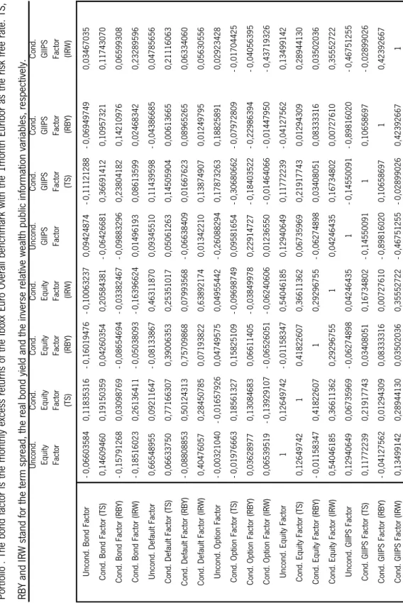
The analysis procedures are very similar to the ones used in the unconditional model. Firstly, I estimated the correlation matrix of the independent variables of my portfolios. The respective results can be seen at the tables 14, 15 and 16 in the Appendix. If it presents values of 1 or -1 it indicates a perfect correlation. The closest to 1 or -1 indicates a stronger correlation of the variables and the closest to 0 indicates a weaker correlation.

Afterwards I tested for multicollinearity by estimating the ‘Variance Inflation Factor’ for each regression model of my portfolios and, as in the unconditional model, I came to the conclusion that there isn’t any multicollinearity issues since all the centered VIF’s values are under 10. These results can be checked at the tables 17, 18 and 19 in the Appendix.

By looking at the Histograms and the Jarque-Bera normality test of the regression residuals in the Figures 6, 8, 9 and 10 in the Appendix I conclude that the regression residuals are not normally distributed. The only portfolio were the regression residuals are normally distributed is the ‘LC Convertible Portfolio’ as it can be seen on the Figure 7 in the Appendix. Results suggest, that I accept the null hypothesis of the skewness being 0 and the kurtosis being 3 of the Jarque-Bera test, the skewness is very close to 0 (- 0,22) and the kurtosis is very close to 3 (3,46). For that reason I cannot reject the null hypothesis that the regression residuals are normally distributed for this portfolio.

Table 3 presents in Panel A the regression estimates of all the portfolios of this dissertation using the conditional model and in Panel B the respective White’s Heteroscedasticity, Breusch-Godfrey Heteroscedasticity and Breusch-Breusch-Godfrey Serial Correlation tests. In Panel A the conditional alphas (α), the conditional coefficients of the different variables (β), levels of significance of each coefficient (by asterisks) and the adjusted coefficient of determination (adj.

average conditional betas of the bond factor, default factor, option factor, equity factor and GIIPS factor, respectively. Each of these factors present several conditional betas when conditioned by the three different public information variables: the term spread (β2, β6, β10, β14 and β18), the real

bond yield (β3, β7, β11, β15 and β19) and the IRW (β4, β8, β12, β16 and β20). In Panel B it’s used the

White (1980) heteroscedasticity test when the portfolios don’t present normal distribution, the Godfrey heteroscedasticity when the portfolios present normality and the Breusch-Godfrey Serial Correlation test. When needed, standard errors are corrected for the presence of heteroscedasticity, using the correction procedure of White (1980), or for the presence of heteroscedasticity and serial correlation using the correction method of Newey and West (1994).

TA BL E 3. Regr essio n Estima tes, H eter osc ed ast icit y an d Se ria l Co rrela tio n t ests u sing th e c on dit io na l 5-fac to r m od el ima tes α0p α1p α2p α3p β 1p β 2p β 3p β 4p β 5p β 6p β7p β8p - 0 ,0 75 ** * 0,0 58 * - 0 ,0 08 - 0 ,0 68 0,7 53 89 ** * - 0 ,0 04 23 - 0 ,0 18 53 * 0,2 10 36 0,1 12 56 ** * 0,0 10 40 - 0 ,0 25 34 ** * - 0 ,1 00 22 ** * - 0 ,1 82 ** * 0,0 98 0,0 09 - 0 ,2 11 0,4 12 72 ** * 0,0 57 84 - 0 ,0 85 78 * 2,0 03 64 ** * 0,2 15 95 ** * 0,0 08 68 - 0 ,0 83 99 ** * 0,2 08 60 - 0 ,0 98 ** * 0,0 28 - 0 ,0 36 ** - 0 ,0 51 0,8 99 24 ** * - 0 ,0 17 76 0,0 09 46 - 0 ,2 15 47 0,0 79 24 ** * 0,0 18 24 - 0 ,0 14 34 - 0 ,2 01 20 ** * - 0 ,0 57 ** * 0,0 32 0,0 09 * 0,0 79 0,7 53 13 ** * - 0 ,0 09 04 - 0 ,0 02 23 - 0 ,0 30 87 0,0 12 34 ** - 0 ,0 07 99 - 0 ,0 01 85 - 0 ,0 48 63 ** - 0 ,0 58 ** * 0,0 52 - 0 ,0 08 - 0 ,1 22 0,7 36 43 ** * 0,0 04 10 - 0 ,0 03 53 0,1 78 32 0,1 27 38 ** * 0,0 10 22 - 0 ,0 24 88 ** * - 0 ,0 79 52 ** β9p β10p β11p β12p β13p β14p β15p β16p β17p β18p β19p β20p Ad j. R 2 0,0 14 24 0,0 26 45 0,0 09 61 0,2 72 80 0,0 32 68 ** * 0,0 06 86 0,0 03 41 0,0 14 45 0,0 00 36 0,0 03 91 0,0 04 19 0,0 26 50 0,9 71 65 0,0 14 75 0,2 79 62 - 0 ,0 38 12 - 1 ,1 28 93 * 0,3 35 66 ** * - 0 ,0 07 51 0,0 26 64 * - 0 ,5 34 42 ** * 0,0 68 67 0,0 12 25 0,0 49 39 - 0 ,3 15 52 0,8 97 89 - 0 ,0 75 46 - 0 ,0 14 15 0,0 16 95 0,5 09 36 ** 0,0 16 08 ** 0,0 07 81 0,0 12 62 ** 0,1 33 12 ** * 0,0 04 67 - 0 ,0 26 55 0,0 02 43 - 0 ,0 42 58 0,9 43 67 0,0 21 45 0,0 18 26 0,0 09 12 0,0 37 29 0,0 00 06 0,0 14 64 ** * - 0 ,0 00 71 0,0 23 76 * - 0 ,0 18 88 - 0 ,0 14 85 0,0 01 70 - 0 ,3 14 95 ** * 0,9 84 80 0,0 09 23 0,0 20 87 0,0 24 31 0,3 67 50 * 0,0 15 58 ** * 0,0 05 00 0,0 00 59 0,0 15 83 0,0 03 56 0,0 16 34 0,0 01 48 0,1 60 60 0,9 65 96 sig nif ica nt a t 5% lev el, * si gn ific an t a t 10% lev el ent t he a vera ge con di tion al a lfa a nd b et as ceda st icity , B re us ch -Godfr ey Het er os ceda st icity an d B re us ch -Godfr ey Serial Correl at ion T es ts W hi te H et er os ce da st ic ity T es t Br eu sc h-Go df re y H et er os ce da st ic ity T es t Br eu sc h-Go df re y Se ria l C or re la tio n Te st 0,0 00 3 -0,1 08 7 -0,0 40 7 0,9 30 5 0,9 97 4 -0,4 08 2 0,0 00 0 -0,0 04 1 0,0 00 1 -0,1 24 7 e resp ec tiv e tes ts' p-valu es 5% w e ca nn ot rej ec t t he n ull h yp ot hesi s on est im at es usi ng th e co ndi tion al 5-fa ct or m odel fo r fiv e eq ua lly weigh ted po rtf oli os of SR Ib on d fu nds , crea ted ac co rd ing to th e va riabl e 'L ip per Global Cl ass ific at ion '. Th e tim e peri od of th is an alysi s is fro m 2018. Th e co ndi tion al alp ha (α )exp res sed in perc enta ge, th e co ndi tion al co ef fic ient s of th e di fferent fa ct ors (β ), th e lev els of sig nif ica nc e of ea ch co ef fic ient (by ast eri sk s) an d th e adj ust ed co ef fic ient of det erm ina tion e benchm ark s used fo r ea ch po rtf oli o are th e sa m e as in th e prev iou s un co ndi tion al m odel . Th e α0 st an d fo r th e av era ge co ndi tion al alp ha an d th e α1 ,α2 an d α3 st an ds fo r th e co ndi tion al alp ha s res pec tiv ely pu bli c inform at ion :a term sp rea d, a rea lb on d yiel d an d an inv ers e rel at ive wea lth (IR W ). Th e β1 ,β5 ,β9 ,β13 an d β17 st an ds fo rt he av era ge co ndi tion al bet as of th e bo nd fa ct or, def au lt fa ct or, op tion fa ct or, eq uit tiv ely. Ea ch of th ese fa ct ors pres ent sev era lc on di tion al bet as wh en co ndi tion ed by th e th ree di fferent pu bli c inform at ion va riabl es: th e term sp rea d (β2 ,β6 ,β10 ,β14 an d β18 ), th e rea lb on d yiel d (β3 ,β7 ,β11 ,β15 an ,β16 an d β20 ). Pa nel B pres ents th e W hit e (1 980) het erosce dast icit y test wh en th e po rtf oli os don ’t pres ent no rm al di st rib ut ion ,t he Breusch-Go df rey het erosce dast icit y test wh en th e po rtf oli os pres ent no rm ali ty an at ion test .S ta ndard errors are co rrec ted, wh en suit ab le, fo rt he pres ence of het erosce dast icit y usi ng th e co rrec tion pro cedure of W hit e (1 980) ,or fo rt he pres ence of het erosce dast icit y an d ser ial co rrel at ion usi ng a nd W est (1 994) .

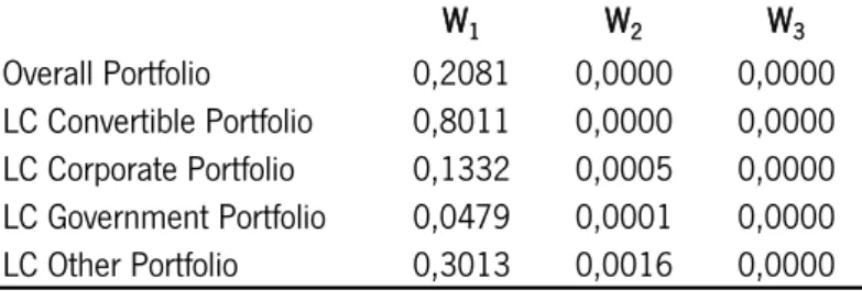
After estimating the conditional model I applied the Wald test developed by Newey and West (1987), presented in table 4, to check for the existence of time-varying alphas, time-varying betas and the joint time-variation of alfas and betas. W1, W2 and W3 correspond to their respective

p-values. At a 5% level of significance, the Wald test results indicates that only in the ‘LC Government Portfolio’ I was able to reject the null hypothesis that the conditional alphas are jointly equal to zero and therefore only this portfolio exhibits time-varying alphas. In spite of not having time-varying alphas for the rest of my portfolios, when testing for time-varying betas and joint time-variation of alphas and betas I was able to conclude the presence of both in every portfolio I am studying. Therefore these results support the application of the conditional model.

The results of Panel A of table 3 show that, for all the portfolios, the lowest adjusted R2 is

89,7% (LC Convertible Portfolio) and the highest is 97,1% (Overall Portfolio) and therefore I can assume that the conditional model is well explained by its independent variables. In agreement to the empirical evidence, the incorporation of conditioning information increases the explanatory power of the model for every portfolio in comparison to the unconditional analysis.

In the unconditional model the alphas of all the portfolios, excluding the ‘LC Convertible Portfolio’ and the ‘LC Other Portfolio’, presented statistically significant negative alphas. The conditional model results show that all the portfolios provide statistically significant negative alphas (α0), at a 5% level of significance, which goes in line with the empirical evidence that the

conditional model provides more robust results. In the other hand, the conditional alphas are slightly lower than the unconditional alphas. These results are not in line with the empirical evidence that the conditional model leads to a slightly higher performance measures. Therefore I will conclude that these portfolios underperform over the analyzed period.

TABLE 4. Wald Test of Newey and West (1987)

W1 W2 W3 Overall Portfolio 0,2081 0,0000 0,0000 LC Convertible Portfolio 0,8011 0,0000 0,0000 LC Corporate Portfolio 0,1332 0,0005 0,0000 LC Government Portfolio 0,0479 0,0001 0,0000 LC Other Portfolio 0,3013 0,0016 0,0000

The Wald test is computed to check for the existence of time-varying alphas, time-varying betas and the joint time-variation of alfas and betas. W1, W2 and W3 correspond to their respective p-values.

Interpreting the average benchmarks coefficients, at a 5% level of significance, for all the portfolios I only found significant betas for the bond factor, default factor and equity factor (with the exception of the ‘LC Government Portfolio’ for this last factor). The betas’ exposures inferences of this model are the same as in the unconditional model.

Analyzing the conditioned alphas (α1, α2 and α3), at a 5% level of significance, only the ‘LC

Corporate Portfolio’ provides a significant alpha when conditioned by the real bond yield information variable. Therefore I can assume a low variability of my conditioned alphas.

Now I will focus on exposing the results of the conditioned benchmarks coefficients, at a 5% level of significance. For the ‘Overall Portfolio’ the results show significant betas for the default factor conditioned by both the real bond yield and the IRW information variables. Considering the ‘LC Convertible Portfolio’, there are significant betas for the bond factor conditioned by the IRW information variable, for the default factor conditioned by the real bond yield information variable and for the equity factor conditioned by the IRW information variable. Looking at the ‘LC Corporate Portfolio’, the results indicate significant betas for the default factor conditioned by the IRW information variable, for the option factor conditioned by the IRW information variable and for the equity factor conditioned by both the real bond yield and IRW information variables. In the ‘LC Government Portfolio’ I found significant betas for the default factor conditioned by the IRW information variable, for the equity factor conditioned by the term spread information variable and for the GIIPS factor conditioned by the IRW information variable. Finally, analyzing the ‘LC Other Portfolio’, results display significant betas for the default factor conditioned by both the real bond yield and the IRW information variables.

The results of the conditioned alphas and betas are in line with the Wald test results, in table 4, where I concluded that this model doesn’t provide time-varying alphas but the presence of time-varying betas is strong.

Interpreting the results of Panel B, in the ‘Overall Portfolio’ by performing a White’s Heteroscedasticity test I reject the null hypothesis of homoscedasticity and by estimating a Breusch-Godfrey Serial Correlation test I was able to accept the null hypothesis of no serial

method. In the ‘LC Corporate Portfolio’ I was able to accept the null hypothesis in both tests and therefore no corrections were needed. Finally, in the ‘LC Government Portfolio’ the results of the heteroscedasticity and serial correlation tests showed me that I had to reject the null hypothesis of homoscedasticity and no serial correlation, respectively. As a result of that I applied the Newey-West (HAC) correction method.

To corroborate my results in table 3 I decided to evaluate the fund’s performance at an individual level as it can be seen at table 5. By interpreting the results I can see that the majority of my funds present negative alphas. Also, regarding only the negative alphas, results show that for the funds in the ‘Overall Portfolio’, ‘LC Convertible Portfolio’, ‘LC Corporate Portfolio’, ‘LC Government Portfolio’ and the ‘LC Other Portfolio’ I have 32,4%, 41,6%, 32,9%, 37,6% and 35,1% of statistically significant alphas, respectively. This analysis supports my findings on the portfolio’s performance evaluation where, for all the portfolios, I found statistically significant negative alphas at a 5% level of significance.

Finally by looking at the empirical evidence on the performance evaluation of SRI bond funds using the conditional multi-factor model I can only compare my results with the pioneer study of Leite and Cortez (2018). My conclusions go in line with this study and the similar financial performance estimates can be justified since I used the same extended multi-factor model, following the four-factor model developed by Elton et al. (1995) and the same public information variables, following Ilmanen, (1995); Silva et al. (2003) and Ayadi and Kryzanowski (2011).

TABLE 5. Individual Fund Performance using the Conditional Model

Positive Alphas (α) Negative Alphas (α)

Overall Portfolio 110 (8) 285 (128)

LC Convertible Portfolio 5 (0) 19 (10)

LC Corporate Portfolio 23 (4) 56 (26)

LC Government Portfolio 24 (2) 69 (35)

LC Other Portfolio 54 (8) 145 (70)

The number of negative and positive alphas using the conditional 5-factor model at the individual fund level is presented. In parenthesis the statistically significant (at a 5% level) alphas are reported.

6. Conclusions

In this dissertation I carry out an empirical analysis of the performance evaluation of European SRI fixed-income funds. I chose this theme since most of the empirical evidence on SRI securities focus on the US SRI equity funds market, therefore it’s important to further explore the financial findings on the European SRI fixed-income market.

My dataset consists of 395 SRI funds with a time period spanning from December 1998 to October 2018. In order to better access the performance of my funds according to their characteristics, I decided to create the following portfolios: ‘Overall Portfolio’, ‘LC Convertible Portfolio’, ‘LC Corporate Portfolio’, ‘LC Government Portfolio’ and ‘LC Other Portfolio’.

Regarding my methodology, I started by estimating the traditional measure of performance, the unconditional factor model and used it as a source of comparison to my final multi-factor model, the conditional model developed by Christopherson et al. (1998). The main conclusions of this dissertation will be generated from the conditional model since empirical evidence acknowledges that this model provides more robust results.

In this dissertation I found several limitations that might or might not affect the results. Firstly, when colleting the data I only found active SRI funds since the website www.yourSRI.com only provides this type of funds. Secondly, I wasn’t able to do a comparison with conventional funds since DataStream didn´t provided me the necessary information to select comparable conventional funds. Lastly, because the benchmarks I found only had recorded data since December 1998 I had to consider this in the starting period for analysis.

In the conditional model, I found strong evidence of time-varying betas which support using the conditional model when evaluating the performance of bond funds. In agreement to the empirical evidence, the results show that this model has an improved explanatory power on the returns of my portfolios in comparison to the unconditional analysis because it accounts variances on the state of the economy. Moreover the results indicated that, for the unconditional and conditional model, the factors option and GIIPS are not significant when explaining the returns of my portfolios and therefore are not relevant for my analysis. I added the GIIPS factor,

comparison to the other significant factors, meaning that the excess returns of a bond market benchmark with similar characteristics is the main factor explaining the returns of my portfolios. As reported by the empirical evidence, since the conditional model provided more significant betas I will consider that using a model with conditioning information variables provides more robust performance results. Performance measures in the conditional model illustrated, for all portfolios, slightly lower negative alphas (controversial with the empirical evidence) than in the unconditional model but still, in both models I conclude that an underperformance for all portfolios exists.

Looking at my results we can conclude that by investing in SRI bond funds we incur on a financial sacrifice. This suggests that investing in SRI bonds funds is not a good financial decision. A company or investor who accepts a financial sacrifice on their investment decisions, by being associated with environmental projects increases their reputation, fulfill their social duties, and make this type of investment a viable approach, according to Derwall and Koedijk (2009).

To improve and corroborate the inferences of my dissertation and since the SRI fixed-income market is still not well explored, I suggest further research on the performance of SRI bond funds with the objective of creating more detailed historical financial records of this market and if possible include a comparison with conventional funds on your study; conduct the analysis on a larger time period to approach different states of the economy and better estimate the performance of your funds and/or include active and dead funds to reduce the limitations of your sample.

7. Appendixes

7.1. Unconditional Model

TABLE 6. Correlation Matrix for the Overall Portfolio, LC Convertible Portfolio and LC Other Portfolio

Bond Overall Factor Default Spread Factor Option Factor Equity Factor GIIPS Factor

Bond Overall Factor 1 - 0,20313782 - 0,57320562 - 0,07532967 0,08896437

Default Spread Factor - 0,20313782 1 0,26487817 0,64168996 0,08251160

Option Factor - 0,57320562 0,26487817 1 - 0,00368978 - 0,25740101

Equity Factor - 0,07532967 0,64168996 - 0,00368978 1 0,11826740

GIIPS Factor 0,08896437 0,08251160 - 0,25740101 0,11826740 1

In this table the correlation matrix of the independent variables are presented for the ‘Overall Portfolio’, ‘LC Convertible Portfolio’ and ‘LC Other Portfolio’. The bond factor is the monthly excess returns of the Iboxx Euro Overall benchmark with the 1month Euribor as the risk free rate.

TABLE 7. Correlation Matrix for the Lipper Category Corporate Portfolio

Bond Corporate Factor Default Spread Factor Option Factor Equity Factor GIIPS Factor Bond Corporate Factor 1 0,24467118 -0,21635939 0,23462521 0,04974773

Default Spread Factor 0,24467118 1 0,26487817 0,64168996 0,08251160

Option Factor -0,21635939 0,26487817 1 - 0,00368978 - 0,25740101

Equity Factor 0,23462521 0,64168996 - 0,00368978 1 0,11826740

GIIPS Factor 0,04974773 0,08251160 - 0,25740101 0,11826740 1

In this table the correlation matrix of the independent variables are presented for the ‘LC Corporate Portfolio’. The bond factor is the monthly excess returns of the ICE BofA ML Euro Corporate benchmark with the 1month Euribor as the risk free rate.

TABLE 8. Correlation Matrix for the Lipper Category Government Portfolio

Bond Sovereign Factor Default Spread Factor Option Factor Equity Factor GIIPS Factor Bond Sovereign Factor 1 - 0,30743069 - 0,67688204 - 0,13329636 0,10903479 Default Spread Factor - 0,30743069 1 0,26487817 0,64168996 0,08251160

Option Factor - 0,67688204 0,26487817 1 - 0,00368978 - 0,25740101

Equity Factor - 0,13329636 0,64168996 - 0,00368978 1 0,11826740

GIIPS Factor 0,10903479 0,08251160 - 0,25740101 0,11826740 1

In this table the correlation matrix of the independent variables are presented for the ‘LC Government Portfolio’. The bond factor is the monthly excess returns of the Iboxx Euro Sovereigns benchmark with the 1month Euribor as the risk free rate.

TABLE 9. Variance Inflation Factors for the Overall Portfolio

Centered VIF

Alpha NA

Bond Overall Factor 1,551863 Default Spread Factor 2,146729 Option Factor 1,967079 Equity Factor 1,655314 GIIPS Factor 1,182535

To test for multicollinearity between the five factors in the regression model of the ‘Overall Portfolio’, the ‘Variance Inflation Factors’ are presented in this table. The bond factor of this portfolio is the monthly excess returns of the Iboxx Euro Overall benchmark with the 1month Euribor as the risk free rate.

TABLE 10. Variance Inflation Factors for the LC Convertible Portfolio

Centered VIF

Alpha NA

Bond Overall Factor 1,641717 Default Spread Factor 2,876649 Option Factor 2,423664 Equity Factor 1,820891 GIIPS Factor 1,354312

To test for multicollinearity between the five factors in the regression model of the ‘LC Convertible Portfolio’, the ‘Variance Inflation Factors’ are presented in this table. The bond factor of this portfolio is the monthly excess returns of the Iboxx Euro Overall benchmark with the 1month Euribor as the risk free rate.

TABLE 11. Variance Inflation Factors for the LC Corporate Portfolio

Centered VIF

Alpha NA

Bond Corporate Factor 1,175647 Default Spread Factor 2,065817 Option Factor 1,34898 Equity Factor 1,802379

GIIPS Factor 1,104475

To test for multicollinearity between the five factors in the regression model of the ‘LC Corporate Portfolio’, the ‘Variance Inflation Factors’ are presented in this table. The bond factor is the monthly excess returns of the ICE BofA ML Euro Corporate benchmark with the 1month Euribor as the risk free rate.

TABLE 12. Variance Inflation Factors for the LC Government Portfolio

Centered VIF

Alpha NA

Bond Sovereign Factor 2,182685 Default Spread Factor 3,032998 Option Factor 2,235009 Equity Factor 1,969707 GIIPS Factor 1,322588

To test for multicollinearity between the five factors in the regression model of the ‘LC Government Portfolio’, the ‘Variance Inflation Factors’ are presented in this table. The bond factor is the monthly excess returns of the Iboxx Euro Sovereigns benchmark with the 1month Euribor as the risk free rate.

TABLE 13. Variance Inflation Factors for the LC Other Portfolio

Centered VIF

Alpha NA

Bond Overall Factor 1,508836

Default Spread Factor 1,958324

Option Factor 1,757511

Equity Factor 1,808141

GIIPS Factor 1,104529

To test for multicollinearity between the five factors in the regression model of the ‘LC Other Portfolio’, the ‘Variance Inflation Factors’ are presented in this table. The bond factor of this portfolio is the monthly excess returns of the Iboxx Euro Overall benchmark with the 1month Euribor as the risk free rate.

FIGURE 1. Histogram and Normality test of regression residuals for the Overall Portfolio

Skewness -1,2571 Kurtosis 8,1546 Jarque-Bera 326,1803

P-value 0,00000

In this table I can check the Histogram and Jarque-Bera normality test of the regression residuals for the ‘Overall Portfolio’. The bond factor of this portfolio is the monthly excess returns of the Iboxx Euro Overall benchmark with the 1month Euribor as the risk free rate.

FIGURE 2. Histogram and Normality test of the regression residuals for the LC Convertible Portfolio

Skewness 0,4100 Kurtosis 4,7724 Jarque-Bera 37,8247

P-value 0,00000

In this table I can check the Histogram and Jarque-Bera normality test of the regression residuals for the ‘LC Convertible Portfolio’. The bond factor of this portfolio is the monthly excess returns of the Iboxx Euro Overall benchmark with the 1month Euribor as the risk free rate.

FIGURE 3. Histogram and Normality test of the regression residuals for the LC Corporate Portfolio

Skewness -0,5316 Kurtosis 14,4781 Jarque-Bera 1317,712

P-value 0,00000

In this table I can check the Histogram, Jarque-Bera normality test of the regression residuals for the ‘LC Corporate Portfolio’. The bond factor is the monthly excess returns of the ICE BofA ML Euro Corporate benchmark with the 1month Euribor as the risk free rate.

FIGURE 4. Histogram and Normality test of the regression residuals for the LC Government Portfolio

Skewness 0,0233 Kurtosis 4,4357 Jarque-Bera 20,4632

P-value 0,00003

In this table I can check the Histogram, Jarque-Bera normality test of the regression residuals for the ‘LC Government Portfolio’. The bond factor is the monthly excess returns of the Iboxx Euro Sovereigns benchmark with the 1month Euribor as the risk free rate.

FIGURE 5. Histogram and Normality test of the regression residuals for the LC Other Portfolio

Skewness -2,4747 Kurtosis 18,9715 Jarque-Bera 2772,587

P-value 0,00000

In this table I can check the Histogram, Jarque-Bera normality test of the regression residuals for the ‘LC Other Portfolio’. The bond factor of this portfolio is the monthly excess returns of the Iboxx Euro Overall benchmark with the 1month Euribor as the risk free rate.

7.2. Conditional Model ) C orr el at ion Ma tri x for th e O ve rall Por tfol io, LC C on ve rtible P ort fol io an d LC O th er Por tfol io Unc ond. Bo nd F ac to r Co nd. Bo nd Fa ct or (T S) Co nd. Bo nd Fa ct or (R BY ) Co nd. Bo nd Fa ct or (IR W) Unc ond. Def ault Fa ct or Co nd. Def ault Fa ct or (T S) Co nd. Def ault Fa ct or (R BY ) Co nd. Def ault Fa ct or (IR W) Unc ond. Opt io n Fa ct or Co nd. Opt io n Fa ct or (T S) Co nd. Opt io n Fa ct or (R BY ) Co nd. Opt io n Fa ct or (IR W) 1 - 0,138 85249 - 0,364 99428 0,12396409 - 0,244 96158 0,11792409 0,04729547 - 0,072 79473 - 0,621 60242 0,23459217 0,45660837 - 0,064 07554 - 0,138 85249 1 0,49203908 0,06529557 0,20904408 0,14265442 0,05385807 0,16583015 0,29352179 - 0,432 05768 - 0,301 43964 0,01975704 ) - 0,364 99428 0,49203908 1 0,13790159 0,05241120 0,03699458 - 0,134 31993 0,03561928 0,52466225 - 0,286 03838 - 0,596 91985 0,03565937 0,12396409 0,06529557 0,13790159 1 - 0,113 25288 0,18535652 0,06141818 - 0,269 76845 - 0,076 08902 0,01144765 0,03294638 - 0,616 15641 r - 0,244 96158 0,20904408 0,05241120 - 0,113 25288 1 0,13807285 - 0,183 17190 0,71677593 0,31452295 0,03676719 - 0,066 91258 0,26164027 ) 0,11792409 0,14265442 0,03699458 0,18535652 0,13807285 1 0,63240227 0,24558791 0,03256509 0,42975108 0,19117389 - 0,016 26017 ) 0,04729547 0,05385807 - 0,134 31993 0,06141818 - 0,183 17190 0,63240227 1 - 0,054 85962 - 0,079 14724 0,29613205 0,24019306 - 0,086 41451 W) - 0,072 79473 0,16583015 0,03561928 - 0,269 76845 0,71677593 0,24558791 - 0,054 85962 1 0,17469049 - 0,017 19248 - 0,048 84234 0,42728690 - 0,621 60242 0,29352179 0,52466225 - 0,076 08902 0,31452295 0,03256509 - 0,079 14724 0,17469049 1 - 0,095 06345 - 0,690 224 0,20217592 ) 0,23459217 - 0,432 05768 - 0,286 03838 0,01144765 0,03676719 0,42975108 0,29613205 - 0,017 19248 - 0,095 06345 1 0,54119673 0,13064175 ) 0,45660837 - 0,301 43964 - 0,596 91985 0,03294638 - 0,066 91258 0,19117389 0,24019306 - 0,048 84234 - 0,690 224 0,54119673 1 - 0,006 81556 W) - 0,064 07554 0,01975704 0,03565937 - 0,616 15641 0,26164027 - 0,016 26017 - 0,086 41451 0,42728690 0,20217592 0,13064175 - 0,006 81556 1 - 0,066 03584 0,14609460 - 0,157 91268 - 0,185 16023 0,66548955 0,06633750 - 0,088 08853 0,40476057 - 0,003 21040 - 0,019 76663 0,03628977 0,06539519 0,11835316 0,19150359 0,03098769 0,26136411 0,09211647 0,77166307 0,50124313 0,28450785 - 0,016 57926 0,18561327 0,13084683 - 0,139 29107 ) - 0,160 19476 0,04260354 - 0,086 54694 - 0,050 38093 - 0,081 33867 0,39006353 0,75709868 0,07193822 0,04749575 0,15825109 0,06611405 - 0,065 26051 - 0,100 63237 0,20584381 - 0,033 82467 - 0,163 96624 0,46311870 0,25351017 0,07993568 0,63892174 0,04955442 - 0,096 98749 - 0,038 49978 - 0,062 40606 0,09424874 - 0,064 26681 - 0,098 83296 0,01496193 0,09345510 0,05061263 - 0,066 38409 0,01342210 - 0,260 88294 0,09581654 0,22914727 0,01236550 ) - 0,111 21288 0,36691412 0,23804182 0,08613599 0,11439598 0,14505904 0,01667623 0,13874907 0,17873263 - 0,306 80662 - 0,184 03522 - 0,014 64066 ) - 0,069 49749 0,10957321 0,14210976 0,02468342 - 0,043 86685 0,00613665 0,08965265 0,01249795 0,18825891 - 0,079 72809 - 0,229 86394 - 0,014 47950 0,03467035 0,11743070 0,06599308 0,23289596 0,04785656 0,21116063 0,06334060 0,05630556 0,02923428 - 0,017 04425 - 0,040 56395 - 0,437 19326 at io n m at rix of th e in depen den tvar ia bles are pres en ted fo r th e ‘O ve ra ll Po rtf olio ’, ‘L C Co nve rtible Po rtf olio ’a nd ‘L C Ot her Po rtf olio ’. Th e bo nd fa ct or is th e m on th ly Ibo xx Eu ro Ove ra ll ben ch m ark with th e 1m on th Eu rib or as th e risk free ra te. TS ,RBY an d IR W st an d fo rt he term sp rea d, th e rea lbo nd yie ld an d th e in ve rse rela tive io n var ia bles , res pec tive ly.