Controller Placement in Software Defined Networking

(1)

UNIVERSIDADE DO ALGARVE

Controller Placement in Software Defined Networking

Mohammad Ashrafi Habibabadi

Master Thesis in Computer Science Engineering

Work done under the supervision of: Prof. Dra. No´elia Correia

(2)

Statement of Originality

Controller Placement in Software Defined Networking

Statement of authorship: The work presented in this thesis is, to the best of my knowledge and belief, original, except as acknowledged in the text. The material has not been submitted, either in whole or in part, for a degree at this or any other university.

Candidate:

———————————

(Mohammad Ashrafi Habibabadi)

Copyright c Mohammad Ashrafi Habibabadi. A Universidade do Algarve tem o

direito, perp´etuo e sem limites geogr´aficos, de arquivar e publicitar este trabalho

atrav´es de exemplares impressos reproduzidos em papel ou de forma digital, ou por

qualquer outro meio conhecido ou que venha a ser inventado, de o divulgar atrav´es

de repositórios cient´ıficos e de admitir a sua cópia e distribui¸cão com objetivos

educacionais ou de investiga¸cão, não comerciais, desde que seja dado crédito ao

(3)

N e t w o r k i n g

Work done at Research Center of Electronics Optoelectronics and Telecommunications (CEOT)

(4)

Abstract

This work focuses on the placement of controllers in software defined networking architectures. The goal is to optimize the latency besides having reliability and scalability in mind. Two mathematical models are proposed, the former determines the optimal controller location in single mapping scenarios and the latter determines the optimal location in multiple mapping scenarios. A scalability factor is introduced to equally decrease load among controllers, increasing the load to capacity gap at controllers in any failure scenario. The results show that the model finds the optimal location while taking redundancy and scalability into consideration.

(5)

Resumo

Este trabalho incide sobre a coloca¸c˜ao de controladores em redes definidas por

soft-ware. O objetivo é otimizar a latência, tendo em considera¸cão a prote¸cão em cenários

de falha e a escalabilidade. S˜ao propostos dois modelos matem´aticos: o primeiro

de-termina a localiza¸cão do controlador em cenários de mapeamento único(single

map-ping), e o último determina a localiza¸cão ideal em cenários de mapeamento múltiplo.

´

E introduzido um fator de escalabilidade para reduzir de igual forma, a carga nos controladores, havendo uma maior diferen¸ca entre a carga nos controladores e a

sua capacidades, isto para qualquer cen´ario de falha. Os resultados mostram que o

modelo consegue encontrar a localiza¸cão ideal tomando em considera¸cão a prote¸cão

em cen´arios de falha e a escalabilidade.

(6)

Acknowledgements

I would like to thank Prof. No´elia for her guidance through all preparation, planning

and development of this thesis. Without her help it would be very difficult to finish this journey. It was a great opportunity to work under her supervision.

I would like to thank Farog Al-Tam for his assistance through all steps required to organize the whole work. His method to solve problems is totally instructive.

(7)

Statement of Originality i Abstract iii Resumo iv Acknowledgements v Nomenclature xi 1 Introduction 1 1.1 SDN . . . 2 1.2 SDN Layers . . . 2 1.3 SDN Architecture . . . 2 1.4 SDN Functionality . . . 3 1.5 Problem Statement . . . 4 1.6 Related Work . . . 5 1.7 Research Objectives . . . 6 1.8 Contributions . . . 6 2 Adopted Methodology 7 2.1 Introduction . . . 7 2.2 Topology . . . 8 2.3 Mapping Scenarios . . . 8 2.4 Remarks . . . 10

3 Controller Placement in SDN - Single Mapping 11 3.1 Mathematical Model . . . 11

3.2 Mathematical Formalization . . . 11

3.2.1 Objective Function: . . . 11

3.2.2 Constraints: . . . 11

4 Controller Placement in SDN - Multiple Mapping 15 4.1 Mathematical Model . . . 15

(8)

4.2 Mathematical Formalization . . . 15

4.2.1 Objective Function . . . 15

4.2.2 Constraints . . . 15

5 Results and Evaluation - Single Mapping 19 5.1 Scenario Setup . . . 19

5.2 Analysis of Results . . . 21

5.3 Conclusions . . . 24

6 Results and Evaluation - Multiple Mapping 25 6.1 Scenario Setup . . . 25

6.2 Analysis of Results . . . 27

6.3 Comparing Multiple Mapping and Single Mapping . . . 30

6.4 Conclusions . . . 32

7 Conclusions and Future Work 33

References 35

A Implementation A-1

A.1 Introduction . . . A-1

(9)

List of Figures

1.1 Functions in networking. . . 1

1.2 SDN Layers: management, control and data planes. . . 3

1.3 SDN Flow. . . 4

2.1 SDN Topology: no failed link. . . 8

2.2 SDN Topology with 1 failed link. . . 8

2.3 SDN Topology with 2 failed links. . . 9

5.1 Physical topologies used for analysis of results in single-mapping ar-chitectures. Large nodes are controllers, medium are switches, and small are non-used locations. Different color indicates switch-controller mapping. . . 20

5.2 Results for Topology I, having high connectivity and relatively low number of possible locations for the controllers, using single-mapping. 22 5.3 Results for Topology II, having high connectivity and relatively low number of possible locations for the controllers, using single-mapping. 23 5.4 Results for Topology III, having high connectivity and relatively low number of possible locations for the controllers, using single-mapping. 24 6.1 Physical topologies used for analysis of results in multiple-mapping architectures. Large nodes are controllers, medium are switches, and small are non-used locations. Different color indicates switch-controller mapping. . . 26

6.2 Results for Topology I, having high connectivity and relatively low number of possible locations for the controllers, using multiple-mapping. 28 6.3 Results for Topology II, having high connectivity and relatively low number of possible locations for the controllers, using multiple-mapping. 29 6.4 Results for Topology III, having high connectivity and relatively low number of possible locations for the controllers, using multiple-mapping. 30 6.5 Scalability factor for Topology I, having high connectivity and rela-tively low number of possible locations for the controllers. . . 31

6.6 Scalability factor for Topology II, having low connectivity and rela-tively low number of possible locations for the controllers. . . 31

(10)

6.7 Scalability factor for Topology III, having low connectivity and

rela-tively high number of possible locations for the controllers. . . 31

7.1 Hypervisor-Based Overlay Networks. . . 34

A.1 General structure of CPLEX solving model. . . A-1

(11)

List of Tables

1.1 SDN enabled switches. . . 4

2.1 Fault tolerance approaches [1]. . . 7

2.2 Failure types and comparison between controllers. . . 7

3.1 Known information for Single Mapping. . . 12

3.2 Required variables for Single Mapping. . . 12

4.1 Known information for Multiple Mapping. . . 16

4.2 Required variables for Multiple Mapping. . . 16

5.1 Input parameters - Single Mapping. . . 21

5.2 Physical topology details - Single Mapping. . . 21

6.1 Input parameters - Multiple Mapping. . . 27

(12)

Nomenclature

SDN Software Defined Networkig

NFV Network Function Virtualization

VTEP VXLAN Tunnel Endpoint

(13)

C H A P T E R

1

Introduction

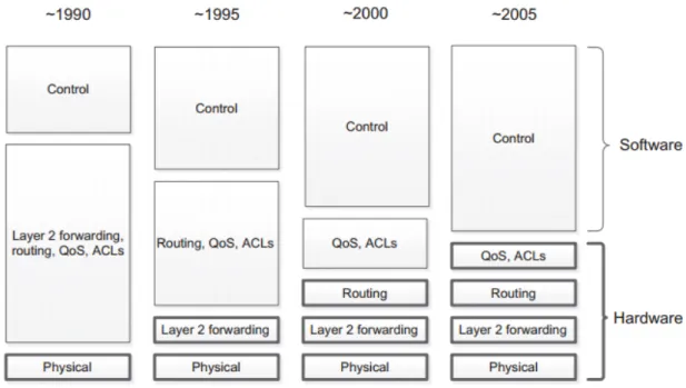
In the beginning of networking it was fairly common to have autonomous devices with all networking functionality built inside it, so the design of small networks was more straightforward. In Figure 1.1 it is easily shown that at the beginning the control and data planes were mostly implemented in software. Then, with the advance of new technologies, hardware became responsible for all data plane tasks while the control plane functionality continued to be done by software. All tasks relating data packet forwarding, in routers or switches, are placed under the data plane, while all tasks related to the overall topology and reachability of the network are placed under the control plane. More recently, Software Defined Networking (SDN) gained a lot of attention.[2]

(14)

1.1 SDN

Software Defined Networking is an emergent paradigm that offers a software-oriented network design, simplifying network management by decoupling the control logic from forwarding devices [3]. The control logic is the brain of the network that decides for best paths, prevents the outage and enforces the business logic into action. This is done in a centralized manner with the help of a computational device (server) instead of using the old distributed design, where every node in the network has the role of finding for best paths or recovering from failures.

1.2 SDN Layers

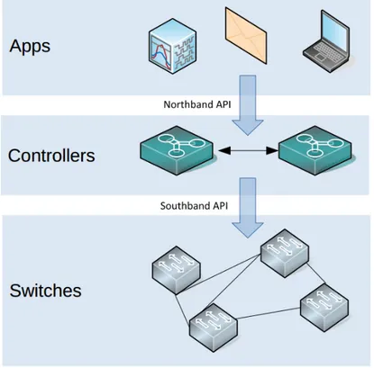
The SDN is composed of three planes: management, control, and data, which are shown in Figure 1.2. The management plane is responsible for defining the network policies, and it is connected to the control plane via northbound interfaces. The brain of SDN is the control plane, which interacts with the data plane using southbound interfaces like OpenFlow [4]. Data plane is mostly responsible of forwarding data packets in switching or routing manner.

In SDN, there are 3 different interfaces:

1. Northbound, a software interface that is responsible for communication be-tween the management application and the controller module.

2. Southbound, a software interface that is responsible for communication be-tween the controller and the networking device.

3. West-East, which is responsible for communication between controllers.

1.3 SDN Architecture

Most of the currently available controllers, like NOX [5] and Beacon [6], are physi-cally centralized. Although a single controller offers a complete network-wide view, it represents a single point of failure and lacks both reliability and scalability [7]. For this reason multi-controller SDNs were developed [4], allowing the control plane to be physically distributed, but maintaining it logically centralized by synchronizing the network state among controllers [1]. Controllers of this type include OpenDay-light [8] and Kandoo [9]. Multi-controller SDNs are able to solve the main problems found in the centralized SDN, but new challenges are introduced, like network state synchronization and switch-controller mappings. Another main problem in multi-controller SDNs is the Controller Placement Problem (CPP) [10]. The problem has

(15)

1.4 SDN Functionality

proved to be NP-hard [11], and is one of the hottest topics in multi-controller SDNs [12, 11, 13, 14].

Figure 1.2: SDN Layers: management, control and data planes.

1.4 SDN Functionality

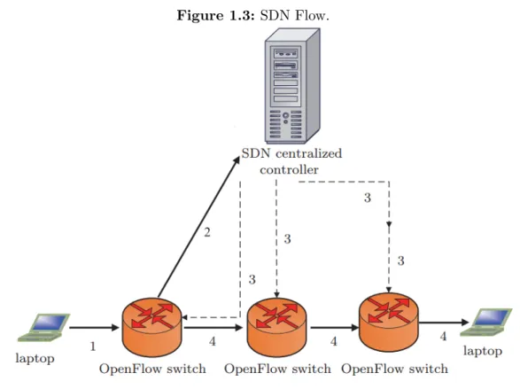
When a switch receives a new packet, it consults its forwarding rules in the flow table in order to determine how to handle the packet. If there is no match in the flow table, the packet is buffered temporarily and the switch initiates a packet-in message to the master controller. Reactively, the controller calculates the path for this packet and installs a new rule in the affected switches. Two major factors that influence the effectiveness of this process are: i) load at the controller; ii) propagation delay

between the switch and the controller. These two constitute a single efficiency

measure: the flow setup time, which will be twice the switch-controller propagation delay plus the queuing and processing time at controllers. The steps performed by a switch and a controller are shown in Figure 1.3. These are the following:

1. The first packet misses the flow-table entry.

2. The flow is forwarded to the controller so that a new flow entry, including an action on the particular flow, can be found.

(16)

1.5 Problem Statement

Figure 1.3: SDN Flow.

4. A new designated flow path.

Nowadays there are SDN enabled products used for different networking land-scapes. Table 1.1 illustrates some of the SDN enabled devices that can be used in different production environments [15].

Table 1.1: SDN enabled switches.

Product Type Description Vendor

Arista 7150 Switch Data center class chasis Arista

CX600 series Router Carrier Class Man Router Huawei

MLX Series Router Service Provider class Brocade

Rackswitch Switch Data center Class Switch IBM

1.5 Problem Statement

As it was mentioned before, one of the main problems in multicontroller SDNs is the Controller Placement Problem (CPP). There are three main questions regarding the controller placement problem [16]:

1. How many controllers are needed? 2. Where should controllers be placed?

(17)

1.6 Related Work

3. Which metrics should be considered?

The main concern in SDN networks is deciding for the number of the controllers, while not letting too many controllers affect the deployment cost. Note, however, that reducing them too much will turn the control plane into a bottleneck.

The second concern in SDN is, therefore, the location of controllers. Network op-erators may plan the controller location from scratch, or may plan for the expansion of the network, usually having cost minimization in mind while meeting the growing number of users and services. In the expansion case this means avoiding disturb-ing the operation of the network. The focus of this work plan is the placement of controllers while considering resilience.

Another concern is the scalability. This is a major concern in any system and it is intensified in SDNs due to the introduction of new control plane traffic (configuration

of switches by controllers). This adds extra concern for controllers which have

to process many requests, forcing researchers to work more on scalability so that networks become more productive.

There are 3 different approaches to tackle the scaling problem in SDN networks. These act, respectively, on: i) data plane, ii) control plane, iii) hybrid [17]. The first approach is to reduce the overloading of controllers by transferring some jobs to forwarding devices. The second approach is to increase the computational power of controllers or use distributed controllers. The last one is the combination of the two previous approaches.

The CPP aims at deciding for the number of required controllers and where to place them [12], partitioning the network into subregions (domains), while consider-ing some quality criteria and cost constraints [13, 18]. The CPP model discussed in this thesis incorporates the previously mentioned flow setup time, while presenting reliable and scalable solutions.

1.6 Related Work

The placement problem was mentioned for the first time in [12]. In fact, this problem is similar to the popular facility location problem, and is solved in the aforementioned article as K-center problem, to minimize the inter-plane propagation delay. In [11] the problem is extended to incorporate the capacity of the controllers. A new metric called expected percentage of control path loss is proposed in [19] to guarantee a reliable model. Cost, controller type, bandwidth, and other factors are considered in [13], and the expansion problem is considered in [14]. The problem is usually modeled in these articles as an integer programming problem.

(18)

1.7 Research Objectives

[21] a game model is also proposed. A comprehensive review of heuristic methods can be found in [22]. QoS-aware CPP is presented in [23] and solved using greedy and network partitioning algorithms. Recently, scalability and reliability issues in large-scale networks are considered in [18]. Clustering and genetic approaches are proposed, but these approaches are prune to sub-optimality.

1.7 Research Objectives

The main goal of this thesis is to define a mathematical model that minimizes metrics related to the deployment of controllers in SDN, while considering the scalability of the network. The work is done in the following steps:

1. Literature review of existing approaches for SDN controller placement prob-lem.

2. Proposal of approaches for controller placement, while considering resilience and scalability, for single-mapping and multiple-mapping cases.

3. Implementation and evaluation proposals.

1.8 Contributions

While in [24] the authors make failure planning in a way to choose backup controllers and minimize two latencies, the latency from switch to the primary controller and to the backup controller, the approach followed in this thesis uses link failure scenarios and then decides for a controller placement that minimizes latency taking all failure scenarios into consideration. Besides such difference regarding protection, the scala-bility is also taken into account. As far as known those two concerns have not been addressed simultaneously in the literature. The single mapping (SM) case is ad-dressed in Chapter 3, while the multiple mapping (MM) case adad-dressed in Chapter 4. Chapters 5 and 6 evaluate the results.

As a result of the first step (SM) a paper has been presented in a conference: • Mohammad Ashrafi, No´elia Correia and Faroq AL-Tam. A Scalable and Reliable Model for the Placement of Controllers in SDN Networks, Broadnet 2018.

(19)

C H A P T E R

2

Adopted Methodology

2.1 Introduction

In the beginning of SDN, every switch was assigned to a single controller (single mapping) but this couldn’t satisfy criteria like load balancing, failover and offload-ing of controllers. For example, to tackle failures different approaches are suggested in Table 2.1, with a brief comparison. Therefore, multiple mapping (each switch mapped to several controllers) is more accepted for tackling failures. In this the-sis two kind of modeling for controller placement are tested: single mapping and multiple mapping. These integer or mixed integer linear programming models are

introduced to CPLEX1 optimizer that solves them.

Table 2.1: Fault tolerance approaches [1].

Mechanism of fault tolerance Fault type Solution

Controller replication Controller fault Ensure the switches-controllers communication without interruption Failure recovery Node or link fault Switches recovery without controllers, recovery time within 50 ms Protection switching Node or link fault Monitoring function, fault recovery time within 50 ms

Segment protection Node or link fault Avoid controllers’ participation in recovery process Fast failover Node or link fault Maximize network resiliency

Packets modification Node or link fault Carry backup route or fault message to change the forwarding policies

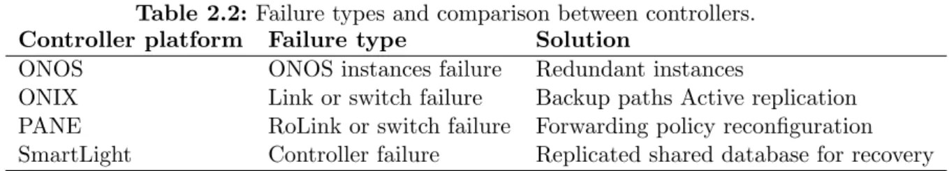
To have a better understanding of how failure is tackled by different controllers, Table 2.2 shows a comparison between different controllers and their capabilities to tackle different kinds of failures.

Table 2.2: Failure types and comparison between controllers.

Controller platform Failure type Solution

ONOS ONOS instances failure Redundant instances

ONIX Link or switch failure Backup paths Active replication

PANE RoLink or switch failure Forwarding policy reconfiguration

SmartLight Controller failure Replicated shared database for recovery

(20)

2.2 Topology

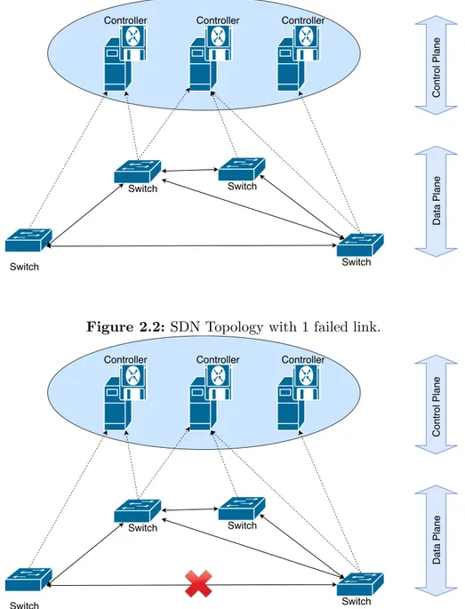
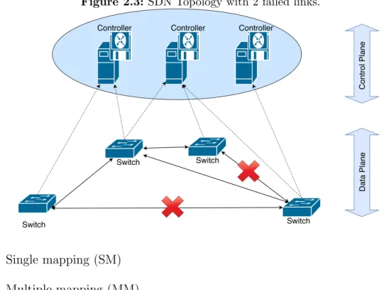
Keeping in mind that we are trying to introduce new metrics like scalability and failover, we have done this by creating different failure scenarios. In each scenario we introduce one or more failing links by removing it from original topology. Please note that switches refer here to layer 3 devices, as is commonly used in the SDN literature.

Figure 2.1: SDN Topology: no failed link.

Control Plane

Data Plane

Switch

Switch Switch

Switch Controller Controller Controller

Figure 2.2: SDN Topology with 1 failed link.

Control Plane

Data Plane

Switch

Switch Switch

2.3 Mapping Scenarios

(21)

2.3 Mapping Scenarios

Figure 2.3: SDN Topology with 2 failed links.

Control Plane

Data Plane

Switch

Switch Switch

1. Single mapping (SM) 2. Multiple mapping (MM)

3. Multiple mapping with overlay topology - future work

For single mapping, every switch is connected to a single controller and there is no load sharing among controllers. The model provided in Chapter 3, whose analysis of results in Chapter 5, fits to single mapping. In Chapter 4, a proposed model for multiple mapping is discussed, which is capable of load sharing between controllers. That is, a single switch is controlled by multiple controllers making this a resilient approach.

Distributed controller is a key concept to tackle the single point of failure issue, making the network more resilient, and in case of failure traffic will flow around the failed node. Controllers reside on physical devices, which are subject to failures, while the software is also subject to failure due to poor design, bugs or overload because of scale [25]. These scenarios enforce the SDN designer to think of a log-ically centralized controller made of one or multiple controllers. The former, as it was mentioned, is a single point of failure which is not accepted in production envi-ronments. The latter will require complex approaches to maintain the global view of the network consistent.

As everybody knows “Many hands make light work.”, and this is exactly how a distributed controller works. It makes handling the load of requests easier compared to single controller, but it will introduce new challenges regarding the location of controllers, controller-switch mapping and delay. The latter is very vital because with high delay, between switch and controller, the overall performance of the

(22)

net-2.4 Remarks

work will decrease and the controller can not respond to requests in a timely manner [26].

2.4 Remarks

In the next chapter, optimal solution models will be found that place controllers on a SDN network or expand an existing one. Besides minimizing the cost of the network, various constrains like flow-setup latency and controller to controller connectivity will also be considered.

(23)

C H A P T E R

3

Controller Placement in SDN - Single

Mapping

3.1 Mathematical Model

In the following discussion the physical topology graph is assumed to be defined by G(N , L), where N is a set of physical nodes/locations and L is a set of physical links. The remaining notation for known information and variables, used through this report, is presented in Tables 3.1 and 3.2, respectively.

3.2 Mathematical Formalization

3.2.1 Objective Function:

To ensure the linear scale up of the SDN network, the goal will be:

Minimize δ + K1

ΘTOTAL

∆ + K2

ΠTOTAL

∆ (3.1)

where ∆ is a big value. The primary goal is to minimize δ, the scalability factor,

and then to reduce latency. The factors K1 and K2 should be adapted according

to switch-controller and inter-controller latency relevance. The motivation behind giving δ more importance is that the provided solution for controller placement will be used for a relatively long period of time, during which traffic conditions may change. Therefore, the scalability of the solution is considered to be critical.

3.2.2 Constraints:

The following additional constraints must be fulfilled. – Placement of controllers:

X

{n∈Nc}

(24)

3.2 Mathematical Formalization

Table 3.1: Known information for Single Mapping.

Term Description

C Set of controllers.

Nc Possible places for controller c ∈ C, Nc⊆ N .

hc Number of requests per second that can be handled by

con-troller c ∈ C.

S Set of switches.

ps Number of requests not matching the lookup table of s ∈ S.

F Set of physical link failure scenarios. Includes a scenario where

all links are up.

Lf Set of physical links failing when scenario f ∈ F occurs.

Table 3.2: Required variables for Single Mapping. Variable Description

σ_nc One if controller c ∈ C is placed at location n ∈ Nc.

µci,cj

ni,nj,f,l One if link l ∈ L\Lf is used for inter-controller ci−cj

commu-nication, located at nodes ni and nj respectively, when failure

f ∈ F occurs. βl

f One if link l ∈ L\Lf is used for inter-controller

communica-tion when failure f ∈ F occurs.

γ_fs,c One if switch s ∈ S is assigned to controller c ∈ C when failure

f ∈ F occur.

λs,c_n,f One if switch s ∈ S is assigned to controller c ∈ C when failure

f ∈ F occurs, and the controller is placed at location n ∈ Nc.

φs,c,ni_f,l One if switch s ∈ S is assigned to controller c ∈ C located at

nodes ni ∈ Nc when failure f ∈ F , and uses link l ∈ L\Lf in

its path.

δ Scalability factor, 0 ≤ δ ≤ 1.

ΘTOTAL _{Total latency, under any failure scenario.}

ΠTOTAL _{Total number of links used, under any failure scenario.}

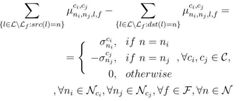
X {l∈L\Lf:src(l)=n} µci,cj ni,nj,f,l− X {l∈L\Lf:dst(l)=n} µci,cj ni,nj,f,l = = ( σ_nci i, if n = ni −σcj nj, if n = nj 0, otherwise , ∀ci, cj ∈ C, ∀f ∈ F , ∀ni ∈ Nci, ∀nj ∈ Ncj, ∀n ∈ N (3.3)

Constraints (3.2) ensure a single location for each controller c ∈ C, while con-straints (3.3) ensure that there will be a path between every pair of controllers, under any failure scenario, while considering their location. These paths are used for state synchronization among controllers.

(25)

among neighboring controllers, if controllers communicate only with its local neigh-bors. Therefore, the paths from any controller, towards all the other controllers, should share as many links as possible (leads to a bus logical topology). This is ensured by the following constraints.

β_fl ≥ µci,cj ni,nj,f,l, ∀ci, cj ∈ C, ∀ni, nj ∈ Nc, ∀f ∈ F , ∀l ∈ L (3.4) ΠTOTAL = X ∀f ∈F X ∀l∈L β_fl × 1/2 (3.5)

where ΠTOTAL_{, counting for the highest number of end-to-end hops in inter-controller}

communication, is to be included in the objective function. – Switch to controller mapping:

X {c∈C} γ_fs,c = 1, ∀s ∈ S, ∀f ∈ F (3.6) X {s∈S} γ_fs,c× ps ≤ hc× δ, ∀c ∈ C, ∀f ∈ F (3.7)

Constraints (3.6) ensure single mapping and constraints (3.7) avoid the overload of controllers, while ensuring scalability regarding future switch migrations (triggered to deal with load fluctuations) due to the use of δ, which is to be included in

the objective function too. Again, the multiple failure scenarios are taken into

consideration. – Switch-controller latency: λs,c_n,f ≥ γs,c_f + σc_n− 1, ∀c ∈ C, ∀n ∈ Nc, ∀f ∈ F , ∀s ∈ S (3.8) X {l∈L\Lf:src(l)=n} φs,c,ni_f,l − X {l∈L\Lf:dst(l)=n} φs,c,ni_f,l = = ( λ s,c n,f, if n = loc(s) −λs,c_n,f, if n = ni 0, otherwise , ∀s ∈ S, ∀c ∈ C, ∀f ∈ F , ∀ni ∈ Nc, ∀n ∈ N (3.9)

Constraints (3.9) ensure switches are placed near to the corresponding controller, and loc(s) is the location of switch s. The total latency is obtained by:

ΘTOTAL = X {s∈S} X {c∈C} X {f ∈F } X {l∈L} X {n∈Nc} φs,c,n_f,l (3.10)

(26)

The ΘTOTAL _{is included in the objective function for latency minimization.}

– Non-negativity assignment to variables:

0 ≤ δ ≤ 1; σ_nc, µci,cj ni,nj,f,l, β l f, γ s,c f , λ s,c n,f, φ s,c,ni f,l ∈ {0, 1}; Θ TOTAL_{, Π}TOTAL_{∈ <}+_{. (3.11)}

This model assumes that the physical layer is not disconnectable under a single

physical link failure. The CPLEX1 _{optimizer has been used to solve the problem}

instances discussed later in Chapter 5.

(27)

C H A P T E R

4

Controller Placement in SDN - Multiple

Mapping

4.1 Mathematical Model

Let us define G(N , L) as the physical topology graph, where N is a set of physical nodes/locations and L is a set of physical links. The remaining notation for known information and variables, used through this report, is presented in Tables 4.1 and 4.2 respectively.

4.2 Mathematical Formalization

4.2.1 Objective Function

To ensure the linear scale up of the SDN network the goal will be:

Minimize δ + K1

ΘMAX

∆ + K2×

ΠMAX

∆ (4.1)

where ∆ is a big value. The primary goal is to minimize δ, and then to reduce

latency. K1 vs K2 should be adapted according to switch-controller and

inter-controller latency relevance.

4.2.2 Constraints

The following additional constraints must be fulfilled. – Placement of controllers:

X

{n∈Nc}

(28)

Table 4.1: Known information for Multiple Mapping.

Term Description

C Set of controllers.

Nc Possible places for controller c ∈ C, Nc⊆ N .

hc Number of requests per second that can be handled by

con-troller c ∈ C.

S Set of switches.

ps Number of requests not matching the lookup table of s ∈ S.

F Set of physical link failure scenarios. Includes a scenario where

all links are up.

Lf Set of physical links failing when scenario f ∈ F occurs.

Table 4.2: Required variables for Multiple Mapping. Variable Description

σ_nc One if controller c ∈ C is placed at location n ∈ Nc.

µci,cj

ni,nj,l,f One if link l ∈ L\Lf is used for inter-controller ci − cj

com-munication, when controllers and placed at ni and nj,

respec-tively, and failure f ∈ F occurs. βl

f One if link l ∈ L\Lf is used for inter-controller

communica-tion when failure f ∈ F occurs.

γ_fs,c Fraction of flow from switch s ∈ S to controller c ∈ C when

failure f ∈ F occurs.

φs,c_f,l Fraction of flow from switch s ∈ S to controller c ∈ C, flowing

at link l ∈ L\Lf when failure f ∈ F occurs.

ω_s,fc,n Fraction of flow arriving to controller c ∈ C, if located at node

n ∈ N , coming from switch s ∈ S when failure f ∈ F occurs.

ΘMAX Highest switch-controller latency, under any failure scenario.

ΠMAX _{Highest number of links used for inter controller}

communica-tion, under any failure scenario.

X {l∈L\Lf:src(l)=n} µci,cj ni,nj,l,f − X {l∈L\Lf:dst(l)=n} µci,cj ni,nj,l,f = = ( σ_nci i, if n = ni −σcj nj, if n = nj 0, otherwise , ∀ci, cj ∈ C, , ∀ni ∈ Nci, ∀nj ∈ Ncj, ∀f ∈ F , ∀n ∈ N (4.3)

Constraints (4.2) ensure a single location for each controller c ∈ C, while con-straints (4.3) ensure that there will be a path between every pair of controllers, under any failure scenario and considering their location. For controllers to communicate just with their local neighbors, the paths from any controller, towards all the other controllers, should share as many links as possible. The following is required:

(29)

4.2 Mathematical Formalization β_fl ≥ µci,cj ni,nj,l,f, ∀ci, cj ∈ C, ∀ni ∈ Nci, ∀nj ∈ Ncj, , ∀l ∈ L, ∀f ∈ F (4.4) ΠMAX ≥ 1 2 X ∀l∈L β_fl, ∀f ∈ F (4.5)

and ΠMAX_{, counting for the highest number of hops between any two controllers,}

should be included in the objective function. – Switch to controller mapping:

X {c∈C} γ_fs,c = 1, ∀s ∈ S, ∀f ∈ F (4.6) X {s∈S} γ_fs,c× ps ≤ hc× δ, ∀c ∈ C, ∀f ∈ F (4.7)

where constraints (4.6) ensure 100% delivery of switch requests to controllers, and constraints (4.7) avoid the overload of controllers, while ensuring scalability regard-ing future multi-mappregard-ing reassignments and/or switch migration (triggered to deal with load fluctuations) due to the inclusion of δ used by the objective function. Again, the multiple failure scenarios are taken into consideration.

– Switch-controller latency: X {l∈L\Lf:src(l)=n} φs,c,ni l,f − X {l∈L\Lf:dst(l)=n} φs,c,ni l,f = = ( ωc,n_s,f, if n = loc(s) −ωc,n_s,f, if n = ni 0, otherwise , ∀s ∈ S, ∀c ∈ C, ∀f ∈ F , , ∀ni ∈ Nc, ∀n ∈ N (4.8)

where loc(s) is the location of switch s. The ω_s,fc,n variables are limited by:

X

{s∈S}

(30)

X

{n∈Nc}

ω_s,fc,n= γ_fs,c, ∀s ∈ S, ∀c ∈ C, ∀f ∈ F (4.10)

Switch-controller communication is ensured, under any failure scenario, accord-ing to placement of controllers. The highest latency is obtained by:

ΘMAX≥ X {l∈L} X {ni∈Nc} φs,c,ni l,f , ∀s ∈ S, ∀c ∈ C, ∀f ∈ F (4.11)

The ΘMAX _{is included at the objective function for latency minimization.}

– Non-negativity assignment to variables:

0 ≤ δ, γ_fs,c, φs,c_f,l, ω_s,fc,n≤ 1; σ_nc, µci,cj f,l , β l f ∈ {0, 1}; Θ MAX , ΠMAX∈ <+. (4.12)

This model assumes that the physical layer is not disconnectable under any single physical link failure.

(31)

C H A P T E R

5

Results and Evaluation - Single Mapping

5.1 Scenario Setup

The values for input parameters, used by the optimizer, are displayed in Table 5.1. Different failure cases were used to evaluate the model under the three topologies shown in Figure 5.1. A case relates to single link failure (no two links fail at the same time in each scenario), while the other relates to multiple link failure scenarios. Two percentages for affected links were tested. More specifically:

Case I: Single link failure scenarios, where ∪f ∈FLf affects a total of 5% (a) or

15% (b) of all the links;

Case II: Two or more links failing simultaneously, in each failure scenario, where

∪f ∈FLf affects a total of 5% (a) or 15% (b) of all the links.

That is, in case Ia 5% of the links may fail, but no two links fail at the same time, while in case IIa there is a 0.5 probability for any two of the failed links to go down at the same time, which may lead to failure scenarios where two or more links fail simultaneously. In cases Ib and IIb, 15% of the links may fail.

(32)

5.1 Scenario Setup

(a) Topology I. #Controllers=2 #Switches=9

(b) Topology II. #Controllers=2 #Switches=9

(c) Topology III. #Controllers=2 #Switches=9

Figure 5.1: Physical topologies used for analysis of results in single-mapping architec-tures. Large nodes are controllers, medium are switches, and small are non-used locations. Different color indicates switch-controller mapping.

(33)

5.2 Analysis of Results

Table 5.1: Input parameters - Single Mapping.

Parameter Value

K1 0.5

K2 0.5

ps [40, 100]

hs [500, 600]

Table 5.2: Physical topology details - Single Mapping.

Topology # Nodes # Links # Possible controller locations

Topology I 21 40 4

Topology II 21 25 4

Topology III 21 25 9

5.2 Analysis of Results

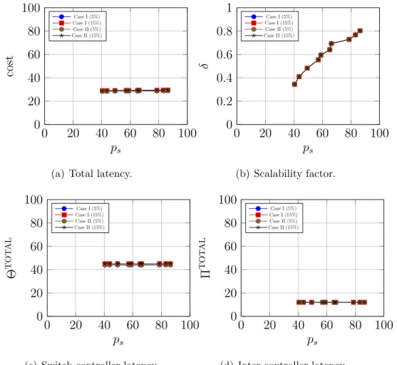
Topology I:

Results for this topology are shown in Figure 5.2. This is the most dense topology, with relatively small number of possible locations for controllers. The scalability factor δ increases linearly as the number of packet-in messages increases , meaning that the gap between controller loads and capacity is reducing due to more

packet-in messages arrivpacket-ing. The latency is relatively low, when compared with other

topologies, because this topology has more links. For different failing scenarios the model presents similar results which is an indicator that the model is able to effectively deal with different failure scenarios.

(34)

5.2 Analysis of Results 0 20 40 60 80 100 0 20 40 60 80 100 ps cost Case I (5%) Case I (15%) Case II (5%) Case II (15%)

(a) Total latency.

0 20 40 60 80 100 0 0.2 0.4 0.6 0.8 1 ps δ Case I (5%) Case I (15%) Case II (5%) Case II (15%) (b) Scalability factor. 0 20 40 60 80 100 0 20 40 60 80 100 ps Θ TOT AL Case I (5%) Case I (15%) Case II (5%) Case II (15%) (c) Switch-controller latency. 0 20 40 60 80 100 0 20 40 60 80 100 ps Π TOT AL Case I (5%) Case I (15%) Case II (5%) Case II (15%) (d) Inter-controller latency.

Figure 5.2: Results for Topology I, having high connectivity and relatively low number of possible locations for the controllers, using single-mapping.

Topology II:

Results for this topology are depicted in Figure 5.3. This topology presents less links than Topology I, but the number of possible locations is kept similar. The main difference regarding these results is that the switch-controller latency has increased while the model keeps the inter-controller communication the same as in Topology I.

(35)

(a) Total latency.

Figure 5.3: Results for Topology II, having high connectivity and relatively low number of possible locations for the controllers, using single-mapping.

Topology III:

Results for this topology are shown in Figure 5.4. This topology also presents less links than Topology I, but the number of possible locations for each controller has increased. In this case it is possible to observe that the total latency significantly decreases due to better results for switch-controller latency. Therefore, the model was able to compensate the reduced number of links, finding adequate places for controllers that lead to lower latency. Results for all scenarios are the same which indicates that the model is able to deal with different failure scenarios without affecting the switch-controller latency, inter-controller latency, and scalability.

(36)

5.3 Conclusions 0 20 40 60 80 100 0 20 40 60 80 100 ps cost Case I (5%) Case I (15%) Case II (5%) Case II (15%)

(a) Total latency.

Figure 5.4: Results for Topology III, having high connectivity and relatively low number of possible locations for the controllers, using single-mapping.

5.3 Conclusions

Results show that scalability is ensured under different failure scenarios, while la-tency increase can be compensated through more freedom in controller’s locations. The model also serves adequately multiple failure scenarios, presenting similar re-sults for more critical failure scenarios and less critical ones.

In general, results show that the model is able to keep scalability (δ) while considering failure scenarios, ensuring load balancing among controllers. The latency may increase when less network connectivity decreases, but this might be avoided if more possible locations for controllers are allowed. Results are similar for Cases Ia, Ib, IIa and IIb, meaning that the model makes a controller placement that serves adequately multiple failure scenarios.

(37)

C H A P T E R

6

Results and Evaluation - Multiple

Mapping

6.1 Scenario Setup

Similarly to single mapping, randomly generated topologies have been used to eval-uate the multiple mapping approach, and these are shown in Figure 6.1. The values for input parameters, used by the optimizer, are displayed in Table 6.1. Different failure cases were used to evaluate the model. A case relates to single link failure (no two links fail at the same time in each scenario), while the other relates to mul-tiple link failure scenarios. Two percentages for affected links were tested. More specifically:

Case I: Single link failure scenarios, where ∪f ∈FLf affects a total of 5% (a) or

15% (b) of all the links;

Case II: Two or more links failing simultaneously, in each failure scenario, where

∪f ∈FLf affects a total of 5% (a) or 15% (b) of all the links.

In case Ia, 5% of the links may fail, but no two links fail at the same time, while in case IIa there is a 0.5 probability for any two of the failed links to go down at the same time, which may lead to failure scenarios where two or more links fail simultaneously. In cases Ib and IIb, 15% of the links may fail.

(38)

6.1 Scenario Setup

(a) Topology I. #Controllers=2 #Switches=9

(b) Topology II. #Controllers=2 #Switches=9

(c) Topology III. #Controllers=2 #Switches=9

Figure 6.1: Physical topologies used for analysis of results in multiple-mapping architec-tures. Large nodes are controllers, medium are switches, and small are non-used locations. Different color indicates switch-controller mapping.

(39)

6.2 Analysis of Results

Table 6.1: Input parameters - Multiple Mapping.

Parameter Value

K1 0.5

K2 0.5

ps [40, 100]

hs [500, 600]

Table 6.2: Physical topology details - Multiple Mapping.

Topology # Nodes # Links # Possible controller locations

Topology I 21 40 4

Topology II 21 25 4

Topology III 21 25 9

6.2 Analysis of Results

Topology I:

Results for this topology are shown in Figure 6.2. This is the most dense topology, with relatively small number of possible locations for controllers. The scalability factor δ increases linearly as the number of packet-in messages increases, meaning that the gap between controller loads and capacity is reducing due to more

packet-in messages arrivpacket-ing. The latency is relatively low, when compared with other

topologies, because this topology has more links. For different failing scenarios the model presents similar results which is an indicator that the model is able to effectively deal with different failure scenarios. But inter-controller communication and switch-controller communication are very low since there are more connection

between devices. For different failing scenarios the model has the same results

which is an indicator that the model is effective under different failure scenarios, while keeping the same latency for inter-controller and switch-controller.

(40)

(a) Total latency.

Figure 6.2: Results for Topology I, having high connectivity and relatively low number of possible locations for the controllers, using multiple-mapping.

Topology II:

Results for this topology are depicted in Figure 6.3. This topology presents less links than Topology I, but the number of possible locations is kept similar. The main difference regarding these results is that the switch-controller latency has increased while the model keeps the inter-controller communication the same as in Topology I. The switch-controller latency has increased because this topology is less dense, although this has not affected inter-controller latency.

(41)

(a) Total latency.

Figure 6.3: Results for Topology II, having high connectivity and relatively low number of possible locations for the controllers, using multiple-mapping.

Topology III:

Results for this topology are shown in Figure 6.4. This topology also presents less links than Topology I, but the number of possible locations for each controller has increased. In this case it is possible to observe that the total latency significantly decreases due to better results for switch-controller latency. Therefore, the model was able to compensate the reduced number of links, by finding adequate places for controllers that lead to lower latency. Results for all scenarios are the same which indicates that the model is adequate to deal with failure scenarios.

(42)

6.3 Comparing Multiple Mapping and Single Mapping 0 20 40 60 80 100 0 20 40 60 80 100 ps cost Case I (5%) Case I (15%) Case II (5%) Case II (15%)

(a) Total latency.

Figure 6.4: Results for Topology III, having high connectivity and relatively low number of possible locations for the controllers, using multiple-mapping.

6.3 Comparing Multiple Mapping and Single

Map-ping

In Figures. 6.5, 6.6, 6.7, it is shown that when a single switch is mapped to multiple controllers, the model is able to find the best placement while distributing switches load between controllers, so scalability factor has more freedom since there is less chance to have overloaded controllers. As a result, the overall performance of the network is optimized.

(43)

6.3 Comparing Multiple Mapping and Single Mapping 0 20 40 60 80 100 0 0.2 0.4 0.6 0.8 1 ps δ Case I (5%) Case I (15%) Case II (5%) Case II (15%)

(a) Multiple Mapping.

0 20 40 60 80 100 0 0.2 0.4 0.6 0.8 1 ps δ Case I (5%) Case I (15%) Case II (5%) Case II (15%) (b) Single Mapping.

Figure 6.5: Scalability factor for Topology I, having high connectivity and relatively low number of possible locations for the controllers.

0 20 40 60 80 100 0 0.2 0.4 0.6 0.8 1 ps δ Case I (5%) Case I (15%) Case II (5%) Case II (15%)

Figure 6.6: Scalability factor for Topology II, having low connectivity and relatively low number of possible locations for the controllers.

0 20 40 60 80 100 0 0.2 0.4 0.6 0.8 1 ps δ Case I (5%) Case I (15%) Case II (5%) Case II (15%)

Figure 6.7: Scalability factor for Topology III, having low connectivity and relatively high number of possible locations for the controllers.

(44)

6.4 Conclusions

The results show that scalability is ensured under different failure scenarios, while latency increase can be compensated through more freedom in controller’s locations. The model also serves adequately multiple failure scenarios, presenting similar re-sults for more critical failure scenarios and less critical ones.

In general, in the multiple mapping case the results show that the model is able to keep scalability (δ) better than single mapping case while considering failure scenarios, ensuring load balancing among controllers. The latency may increase when less network connectivity decreases, but this might be avoided if more possible locations for controllers are allowed. Results are similar for Cases Ia, Ib, IIa and IIb, meaning that the model makes a controller placement that serves adequately multiple failure scenarios.

(45)

C H A P T E R

7

Conclusions and Future Work

Programmable networks, like SDN, are getting more and more attention over the last years. In such kind of architectures, the controllers are the most important elements, and most of the ongoing research focus on different issues about them. One of the most important research topic has to do with finding the best placement for controller, while fulfilling different criteria like latency and/or failover.

In this thesis, a scalable and reliable model for controller placement is introduced. This model is mathematically formulated and optimal solutions for controller place-ment, under different failure scenarios, are obtained. This study tries to find for the best placement while considering failover and scalability. A first mathematical model regarding single mapping scenarios has been implemented, and results have been obtained and analyzed in chapter 5. Results indicate that scalability is en-sured under different failure scenarios while resilience is guaranteed. The second mathematical model regarding multiple mapping is also implemented, and results overcome the ones obtained for single mapping due to the flexible nature of multiple mapping approaches.

Recently, switches implemented as software applications, usually running in con-junction with a hypervisor in a data center rack, have been proposed [26]. Like virtual machines, virtual switches may be instantiated or moved under software control. Therefore, given an existing physical network, the placement of controllers can be planned having switch virtualization into consideration. Such scenarios are to be considered in future work. An issue that must be considered is that when there are multiple controllers, state synchronization is required to keep network in-formation consistent among controllers. One might think that full inter-controller connectivity is the best choice, as in [13], but this brings scaling problems. That is, state synchronization load, to maintain a consistent information state among con-trollers, should be reduced for scalability [28]. In [27] it is stated that the controller load can be reduced, and load balance among neighboring controllers is achieved, if controller needs to communicate only with its local neighbors, within a predefined number of hops. Having this issue in mind, the approach can be to provide a virtual

(46)

Conclusions and Future Work

controller topology (expected connectivity between controllers) for further embed-ding at the physical topology. This way any inter-controller connectivity can be provided as input. Such approach, together with virtual switch instantiation, will allow for physical resources to be efficiently utilized. Figure 7.1 illustrates the use of VXLAN and VTEP technologies to achieve virtual implementation in SDN.

(47)

References

[1] Y. Zhang, L. Cui, W. Wang, and Y. Zhang, “A survey on software defined networking with multiple controllers,” Journal of Network and Computer Ap-plications, vol. 103, pp. 101 – 118, 2018.

[2] P. Goransson and C. Black, “Chapter 2 - why sdn?,” in Software Defined Net-works (P. Goransson and C. Black, eds.), pp. 21 – 35, Boston: Morgan Kauf-mann, 2014.

[3] N. McKeown, T. Anderson, H. Balakrishnan, G. Parulkar, L. Peterson, J. Rex-ford, S. Shenker, and J. Turner, “OpenFlow: Enabling innovation in campus networks,” ACM SIGCOMM COMPUTER COMMUNICATION REVIEW, vol. 38, pp. 69–74, APR 2008.

[4] O. N. Foundation, “Openflow switch specification,” tech. rep., 2011.

[5] N. Gude, T. Koponen, J. Pettit, B. Pfaff, M. Casado, N. McKeown, and S. Shenker, “Nox: Towards an operating system for networks,” SIGCOMM Comput. Commun. Rev., vol. 38, pp. 105–110, July 2008.

[6] D. Erickson, “The beacon openflow controller,” in Proceedings of the Second ACM SIGCOMM Workshop on Hot Topics in Software Defined Networking, HotSDN ’13, (New York, NY, USA), pp. 13–18, ACM, 2013.

[7] S. H. Yeganeh, A. Tootoonchian, and Y. Ganjali, “On Scalability of Software-Defined Networking,” IEEE COMMUNICATIONS MAGAZINE, vol. 51, pp. 136–141, FEB 2013.

[8] J. Medved, A. Tkacik, R. Varga, and K. Gray, “OpenDaylight: Towards a Model-Driven SDN Controller Architecture,” in 2014 IEEE 15TH INTER-NATIONAL SYMPOSIUM ON A WORLD OF WIRELESS, MOBILE AND MULTIMEDIA NETWORKS (WOWMOM), IEEE, 2014.

[9] S. Hassas Yeganeh and Y. Ganjali, “Kandoo: A framework for efficient and scalable offloading of control applications,” in Proceedings of the First Workshop on Hot Topics in Software Defined Networks, HotSDN ’12, (New York, NY, USA), pp. 19–24, ACM, 2012.

(48)

References

[10] P. Vizarreta, C. M. Machuca, and W. Kellerer, “Controller Placement Strate-gies for a Resilient SDN Control Plane,” in PROCEEDINGS OF 2016 8TH IN-TERNATIONAL WORKSHOP ON RESILIENT NETWORKS DESIGN AND MODELING (RNDM) (Jonsson, M and Rak, J and Somani, A and Papadim-itriou, D and Vinel, A, ed.), pp. 253–259, 2016.

[11] G. Yao, J. Bi, Y. Li, and L. Guo, “On the Capacitated Controller Placement Problem in Software Defined Networks,” IEEE COMMUNICATIONS LET-TERS, vol. 18, pp. 1339–1342, AUG 2014.

[12] B. Heller, R. Sherwood, and N. McKeown, “The Controller Placement Prob-lem,” ACM SIGCOMM COMPUTER COMMUNICATION REVIEW, vol. 42, pp. 473–478, OCT 2012.

[13] A. Sallahi and M. St-Hilaire, “Optimal Model for the Controller Placement Problem in Software Defined Networks,” IEEE COMMUNICATIONS LET-TERS, vol. 19, pp. 30–33, JAN 2015.

[14] A. Sallahi and M. St-Hilaire, “Expansion Model for the Controller Placement Problem in Software Defined Networks,” IEEE COMMUNICATIONS LET-TERS, vol. 21, pp. 274–277, FEB 2017.

[15] R. Masoudi and A. Ghaffari, “Software defined networks: A survey,” Journal of Network and Computer Applications, vol. 67, pp. 1 – 25, 2016.

[16] R. El-Azouzi, D. Menasche, E. Sabir, F. De Pellegrini, and M. Benjillali, Ad-vances in Ubiquitous Networking 2: Proceedings of the UNet16. Lecture Notes in Electrical Engineering, Springer Singapore, 2016.

[17] D. Kreutz, F. M. V. Ramos, P. E. Verissimo, C. E. Rothenberg, S. Azodolmolky, and S. Uhlig, “Software-Defined Networking: A Comprehensive Survey,” PRO-CEEDINGS OF THE IEEE, vol. 103, pp. 14–76, JAN 2015.

[18] F. Bannour, S. Souihi, and A. Mellouk, “Scalability and reliability aware sdn controller placement strategies,” in 2017 13th International Conference on Net-work and Service Management (CNSM), pp. 1–4, Nov 2017.

[19] H. Yannan, W. Wendong, G. Xiangyang, Q. Xirong, and C. Shiduan, “On Reliability-optimized Controller Placement for Software-Defined Networks,” CHINA COMMUNICATIONS, vol. 11, pp. 38–54, FEB 2014.

[20] L. Yao, P. Hong, W. Zhang, J. Li, and D. Ni, “Controller Placement and Flow based Dynamic Management Problem towards SDN,” in 2015 IEEE

(49)

References

INTERNATIONAL CONFERENCE ON COMMUNICATION WORKSHOP (ICCW), IEEE International Conference on Communications Workshops, pp. 363–368, IEEE, 2015.

[21] G. Cheng and H. Chen, “Game model for switch migrations in software-defined network,” ELECTRONICS LETTERS, vol. 50, pp. 1699–1700, NOV 6 2014. [22] S. Lange, S. Gebert, T. Zinner, P. Tran-Gia, D. Hock, M. Jarschel, and M.

Hoff-mann, “Heuristic Approaches to the Controller Placement Problem in Large Scale SDN Networks,” IEEE TRANSACTIONS ON NETWORK AND SER-VICE MANAGEMENT, vol. 12, pp. 4–17, MAR 2015.

[23] T. Y. Cheng, M. Wang, and X. Jia, “QoS-Guaranteed Controller Place-ment in SDN,” in 2015 IEEE GLOBAL COMMUNICATIONS CONFERENCE (GLOBECOM), IEEE Global Communications Conference, 2015.

[24] B. P. R. Killi and S. V. Rao, “Controller placement with planning for fail-ures in software defined networks,” in 2016 IEEE International Conference on Advanced Networks and Telecommunications Systems (ANTS), pp. 1–6, Nov 2016.

[25] A. Sallahi, “Optimal placement of controllers in software defined networks,” mathesis, Department of Systems and Computer Engineering, Carleton Uni-versity, May 2014.

[26] P. Gransson, C. Black, and T. Culver, “Chapter 8 - sdn in the data center,” in Software Defined Networks (Second Edition) (P. Gransson, C. Black, and T. Culver, eds.), pp. 191 – 215, Boston: Morgan Kaufmann, second edition ed., 2017.

[27] S. Schmid and J. Suomela, “Exploiting locality in distributed sdn control,” in Proceedings of the Second ACM SIGCOMM Workshop on Hot Topics in Software Defined Networking, HotSDN ’13, (New York, NY, USA), pp. 121– 126, ACM, 2013.

[28] Z. Guo, M. Su, Y. Xu, Z. Duan, L. Wang, S. Hui, and H. J. Chao, “Improving the performance of load balancing in software-defined networks through load variance-based synchronization,” Computer Networks, vol. 68, pp. 95 – 109, 2014. Communications and Networking in the Cloud.

(50)

A P P E N D I X

A

Implementation

A.1 Introduction

The general approach used by CPLEX to solve mathematical models is shown in Figure. A.1. In this thesis, additional steps were required for tests to be performed, whose flowchart is shown in Figure. A.2. It starts with a set of initial inputs which include the existing nodes and switches, number of controllers, together with phys-ical links. A python algorithm builds failure scenarios and adds the corresponding constraints to the base model.

Figure A.1: General structure of CPLEX solving model.

The data model is applied to CPLEX so that the best location for facilities is found by CPLEX solver. Such solver is able to find the global optimal solution.

A.2 Building the Model

(51)

A.2 Building the Model

Figure A.2: Main flow chart of a test (F is the number of scenarios).

• Modeling objects for defining the optimization problem (constraints, objective function, etc.) They are grouped into an IloModel object representing the complete optimization problem.

• Solving objects for problems represented by modeling objects to be solved. A solving object reads a model, extracts its data, solves the problem and answers queries on solution.

In the following, it is shown the modeling object and solving object, respec-tively.

/********************************************* * OPL 12.8.0.0 Model

* Author: Mohammad Ashrafi

* Creation Date: Apr 19, 2018 at 4:34:04 PM *********************************************/ int nSwitches =...; int nLinks =...; int nControllers =...; int nNodes =...; int Number_of_scenario=...;

(52)

A.2 Building the Model float k=50; float DL=100; range nodes=0..nNodes-1; range scenarios=0..Number_of_scenario-1; tuple edge{ int scenario; int source; int dest; } tuple switch{ int loc; float load; } tuple controller{ int id; float capacity; } {int} possible_node= ...; {edge} links=...; {switch} switches=...; {controller} controllers=...;

dvar boolean sigma[controllers][nodes];

dvar boolean mu[controllers][controllers][possible_node][

,→ possible_node][links];

dvar boolean beta[links];

dvar boolean gamma[switches][controllers][scenarios];

dvar boolean phi[switches][controllers][links][possible_node][

,→ scenarios];

dvar boolean lambda [switches][controllers][possible_node][scenarios

,→ ];

dvar float+ delta ; dvar float+ PI; dvar float+ THETA;

(53)

A.2 Building the Model minimize cost ; subject to { //formula (2) forall(c in controllers) node_uniqe: sum(n in possible_node)sigma[c][n]==1; forall(n in possible_node) node_1: sum(c in controllers)sigma[c][n]<=1; //formula (3)

forall(s in scenarios,ci in controllers, cj in controllers,ni in

,→ possible_node,nj in possible_node:

ci.id!=cj.id && ni!=nj ) {

conservation_law_src:

sum(l in links:l.source == ni && l.scenario==s) mu[ci][cj][ni][nj][l]

,→ == sigma[ci][ni] ;

}

forall(s in scenarios,ci in controllers, cj in controllers,ni in

,→ possible_node,nj in possible_node:

ci.id!=cj.id && ni!=nj ) {

conservation_law_dst:

sum(l in links:l.dest == nj && l.scenario==s) mu[ci][cj][ni][nj][l]

,→ == sigma[cj][nj] ;

}

forall(s in scenarios,n in nodes, ci in controllers, cj in

,→ controllers,ni in possible_node,nj

in possible_node: ci.id!=cj.id && n!=nj && n!=ni ) {

conservation_law_int:

(54)

A.2 Building the Model

,→

-sum(l in links:l.dest == n && l.scenario==s ) mu[ci][cj][ni][nj][l]

,→ == 0 ;

}

//formula (4)

forall(s in scenarios,ci in controllers,ni in possible_node,nj in

,→ possible_node,cj

in controllers,l in links:ci!=cj && s==l.scenario) mu[ci][cj][ni][nj][l] <= beta[l];

//formula (5)

/*forall(s in scenarios) loacl_flow:

sum(l in links: s==l.scenario) beta[l] * 0.5 <= PI;*/ //formula (5)

loacl_flow:

sum(s in scenarios,l in links: s==l.scenario) beta[l] * 0.5 == PI;

//formula (6)

forall(s in switches,sc in scenarios) switch_flow:

sum(c in controllers) gamma[s][c][sc] == 1;

//formula (7)

forall(c in controllers,sc in scenarios) controller_load:

sum(s in switches) gamma[s][c][sc] * s.load <= c.capacity * delta ;

//formula (8)

forall(s in switches,n in possible_node,c in controllers,f in

,→ scenarios)

formula8:

lambda[s][c][n][f]>=gamma[s][c][f]+sigma[c][n]-1;

//formula 9

forall(sc in scenarios,nj in possible_node,s in switches, c in

(55)

A.2 Building the Model {

Switch_controller_latency_src:

sum(l in links:l.source == s.loc && sc==l.scenario ) phi[s][c][l][nj

,→ ][sc] ==

lambda[s][c][nj][sc] ;

}

forall(sc in scenarios,nj in possible_node,s in switches, c in

,→ controllers)

{

Switch_controller_latency_dst:

sum(l in links:l.dest == nj && sc==l.scenario) phi[s][c][l][

,→ nj][sc] ==

lambda[s][c][nj][sc] ;

}

forall(sc in scenarios,n in nodes,nj in possible_node,s in switches,

,→ c in controllers:n!=nj

&& n!=s.loc ) {

Switch_controller_latency_int:

sum(l in links:l.source == n && sc==l.scenario) phi[s][c][l][nj][sc]

,→

-sum(l in links:l.dest == n && sc==l.scenario) phi[s][c][l][nj][sc] ==

,→ 0 ;

}

//formula (10

/*forall(c in controllers,s in switches,sc in scenarios) highest_latenacy:

sum(l in links:sc==l.scenario,ni in possible_node) phi[s][c][l][ni][

,→ sc] <= THETA;*/

// formula (10

sum(sc in scenarios,c in controllers,s in switches,ni in

,→ possible_node,l in links:sc==l.scenario)

(56)

A.2 Building the Model }

execute {

var f=new IloOplOutputFile("output.txt"); f.writeln("[vars]");

f.writeln("Number of Nodes = ",nNodes);

f.writeln("Number of controllers = ",nControllers); f.writeln("Number of Switches = ",nSwitches);

f.writeln(""); f.writeln("cost = ",cost); f.writeln("sigma = ",sigma); f.writeln("gamma = ",gamma); f.writeln("switches = ",switches); f.writeln("Theta = ",THETA); f.writeln("Delta = ",delta); f.writeln("PI = ",PI); f.writeln("controllers= ",controllers); f.close(); }

Controller Placement in Software Defined Networking

UNIVERSIDADE DO ALGARVE