Abstract
The floor pan is an important component that connects the front and rear segments of the automotive underbody structure. Global stiff-ness and NVH characteristics of BIW are highly dependent to shape, thickness and mass of the body panels and could be evaluated by modal characteristics of these panels. The feeling of solidness and comfort of passengers in an automotive is also dependent to the modal behavior of the underbody components as well as the floor pan. On the other hand, it is desired to reduce the total mass of the floor pan, in order to have a lighter vehicle with better fuel economy and emission standards. In this paper, the effect of geometrical pa-rameters on natural frequency and total mass of the floor pan of a conventional B-Segment automotive body is investigated using finite element simulation. The finite element model is verified using an experimental test on the floor pan. Taguchi orthogonal array is used to design the numerical experiments. Subsequently, S/N ratio analysis is performed to evaluate the effect of each design variable on the output functions. The panel’s thickness is determined to have the most contribution in affecting the natural frequency and weight using Analysis of Variance (ANOVA). The best combination of geo-metrical variables which leads to the trade-off results is then figured out by a new multi-criteria decision making (MCDM) method devel-oped in this study. Accuracy of this method is verified by comparing the trade-off results with TOPSIS, as a conventional MCDM method.
Keywords
Floor pan, modal, natural frequency, Taguchi, MCDCM, SVCB.
Parametric Modal Study and Optimization of the Floor Pan
of a B-Segment Automotive Using a Hybrid Method
of Taguchi and a Newly Developed MCDM Model
1 INTRODUCTION
Statistics has reported a growing rate of automotive manufacturing in the last two decades Kline
Mohammad Hassan Shojaeefard a,b Abolfazl Khalkhali a,c
Abdolah Tavakoli Lahijani a,d
a Automotive Simulation and Optimal
Design Research Laboratory, School of Automotive Engineering, Iran University of Science and Technology, Tehran, Iran.
b [email protected] c [email protected]
http://dx.doi.org/10.1590/1679-78253189
year in the future years and the production is expected to exceed 100 million vehicles by 2017 Eco-nomic Outlook (2014). This breathtaking volume of production requires an extremely high level of industrial and management technology to remain in the highly competitive market of automotive manufacturing. This is not possible unless they employ efficient design and manufacturing techniques. Today, Computer-Aided Engineering (CAE) is known as a necessary technique which helps the engi-neers to remarkably save time and money in the design and manufacturing process. In the recent years, a wide range of studies have been carried out to develop Finite Element (FE) analyses as alternatives of the experimental conventional procedures of automotive design such as (Noise, Vibra-tion and Harshness) NVH Sobieski et al (2001), safety Shin et al (2012) and strength Palmonella et al (2005).
Stiffness is a crucial attribute in design process of every road vehicle. Previous studies have been carried out to investigate the effects of automotive body stiffness on vehicle dynamic characteristics. These investigations have demonstrated that the overall response of the vehicle is improved with a stiffer body due to stiffer connection between front and rear components Krishnan (2011). The stiffer a road vehicle’s body, the better ride, handling and NVH performance is obtained Chaturved et al (2010). The overall stiffness of a road vehicle depends on the local stiffness of the constituent parts Chaturved et al (2010). Hence, the target of stiffening a vehicle’s body is automatically cascaded to a set of new targets: stiffening the constituent parts of the Body in White (BIW). The overall stiffness of BIW is remarkably affected by the floor panel. This is why the stiffness of this part of automotive body is specially focused by researchers in the last two decades Mohan Kumar et al (2015). A con-ventional approach to judge about stiffness of the floor panel is vibration analysis Mignery (2016). Due to the direct relation between the natural frequencies and stiffness, the higher the natural fre-quency, the stiffer structure of the panel is expected.
Geometric parameters of the floor pan affect the natural frequency and subsequently, the stiffness of this component Suh et al (2007). It is important for automotive design engineers to find information about the effect of each geometrical variable of the floor pan on the natural frequency. Parametric study of the floor pan’s vibration is important from two points of view: 1- Sensitivity of the natural frequencies with respect to each of the geometrical variables; 2- To obtain a set of geometrical varia-bles leading to the highest natural frequencies.
performance and computational cost. Several applications of this method in the engineering optimi-zation problems including aerospace Mathan Kumar (2016), mechanical engineering Parvin Kumar et al (2016) and automotive engineering P. Senthil Kumar (2013) could be found in the literature.
Sun et al (2015) used Taguchi method to explore how to maximize the crashworthiness of the hybrid steel-aluminum tailor welded structures involving uncertainties. The optimal results showed that Taguchi method is successful not only to reduce the peak force, but also to improve the absorbed energy of impact. Furthermore, the robustness of these two indicators was also significantly enhanced. P. Senthil Kumar et al (2013), used Taguchi method for optimizing a vehicle’s suspension system. They presented an optimum concept to design a passenger- friendly vehicle suspension system. Using Analysis of Variance (ANOVA) sensitivity analysis, they also found that the stiffness of absorber and seat spring are the most significant parameters which affect the seat displacement. Wang Mingqi et al (1997) used Taguchi method to maximize the stiffness of a full structure double-decker finite ele-ment model. As a result of this study, they improved the torsional stiffness by 20% and the bending stiffness by 23.3%. This study verified that the Taguchi method is effective in improving the stiffness of a vehicle. But a full road vehicle is made up by more than 300 distinct components which each part’s stiffness is influenced by several geometrical and mechanical parameters. Therefore, it is a cumbersome, time consuming and costly process to optimize the stiffness of all of these components separately. A good approach is to identify the key components which have the most contribution in the global stiffness of the vehicle. One of these key components is the car’s floor pan Mohan Kumar et al (2015).
2 EXPERIMENTAL MODAL ANALYSIS
In this section, details of the modal experiment on the prototype of the research case are reported. The research case is the floor pan of NP01 (Natural platform project), a B-segment automotive prod-uct family which is under development in Automotive department of Iran University of Science and Technology. The aim of this experiment is to validate the results of the FE modeling and simulation (Section 3) with the real values.
2.1 Experiment Specimen
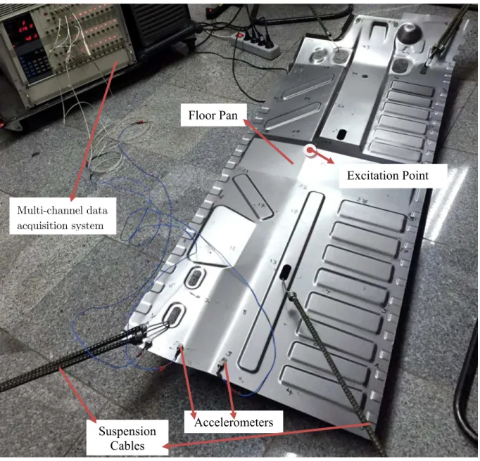
A prototype of the floor pan is produced and submitted to modal experimental test as shown in Figure 1. The fabrication method is stamping by soft tools, drawing operation and trimming is carried out by laser cut. The experiment details are explained as follows.
2.2 Impact Testing
A roving hammer test is the most common type of modal analysis test. An accelerometer is fixed at a Single Degree of Freedom (DOF), and the structure is subjected to impacts at as many DOFs as desired to define the mode shapes of the structure. Using a two channel Fast Fourier Transform (FFT) analyzer, Frequency Response Functions (FRFs) are computed between each impact DOF and the fixed response DOF. A suitable grid is usually marked on the structure to define the impact points.
It is generally impossible to impulse a structure in all three directions at all points, so three-dimensional (3-D) motion cannot be measured at all points. When 3-D motion at all points is desired, a roving tri-axial accelerometer may be used and the structure is excited at a fixed DOF with the hammer. However, tri-axial accelerometers are usually more massive. Since the tri-axial accelerometer must be simultaneously sampled together with the force data, a four-channel FFT analyzer is required. Note, however, that the roving accelerometer presents a different mass-load to the structure at each response site. This can lead to inconsistencies in the data that makes more difficult to find an accurate curve fit.
Figure 1: Modal test setup.
In this research, the charge type hammer has been used to excite the frame. To cover frequency ranges of interest, a rubber tip has been utilized. Excitation point has been selected so that the maximum mode shapes could be obtained (It must not be on the nodal points of any mode of interest). In order to reduce the noises in the measurements, each of the stage results have been obtained by averaging 10 measurements of the same kind.
2.3 Test Equipments
Equipment used during the modal test is listed as below:
Multi-channel data acquisition system, Difa Measuring System, Type ScadasII
Floor Pan
Suspension
Cables
Accelerometers
Multi-channel data acquisition system
Impact Hammer (charge type), Type 8202, B&K
Force Transducer, 208B03, PCB
Tri- directional accelerometers, type 356 A11, PCB
Thermometer, CEWAL CO; Type 11/98-L
Hygrometer, TFA CO.
LMS CADA-X (The post-processing software for the experimental test)/ FMON (Fourier mon-itor module of LMS CADA-X).
LMS CADA-X/ Modal Analysis (The modal analysis module of LMS CADA-X)
2.4 Test Conditions
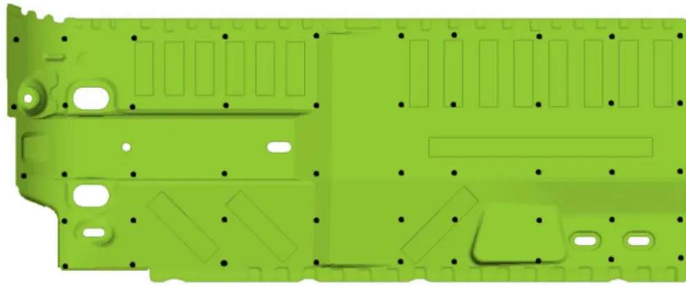
As an overall rule to find the natural frequencies of a system, it is required that the stiffness of suspension be about 10 times higher than the first natural frequency of the system. This matter is checked before any experiment in the modal laboratory Ewins (1984). The frame was suspended using cables having the elasticity suitable enough for the natural mode extraction as depicted in Figure 1. In order to get first 4 natural frequencies of the panel, 48 points were marked on it for accelerometers installation locations. A schematic image of the points where accelerometers are mounted is shown in Figure 2. A geometrical model of the system was created using six coordinates required for each node. Each node corresponds to a point on the panel. The tri-directional accelerometers were attached to these points.
Figure 2: Accelerometers’ positioning points on the floor pan.
2.5 Obtaining Modal Parameters
Here, the most general purpose parameter estimation technique called Time Domain MDOF Analysis has been used LMS theory and background (2000). It provides a complete and accurate modal model from single input multiple output frequency response functions. It uses global estimators; this means that it analyzes all the data records simultaneously in order to estimate the structure’s characteristics. With this approach, a unique estimation of the pole values (natural frequencies) has been obtained.
3 FINITE ELEMENT ANALYSIS
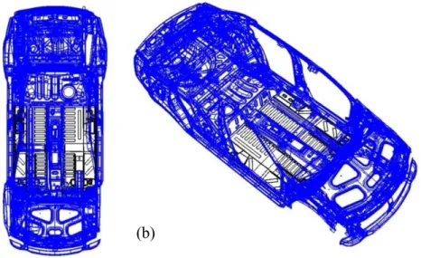
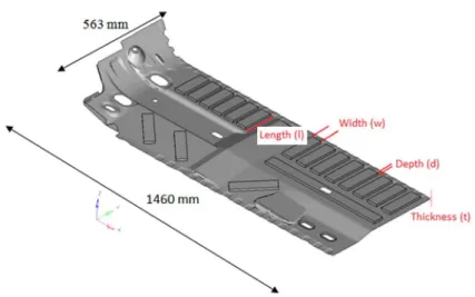
Position of the floor pan in the BIW is shown in Figure 3. Furthermore, the geometrical shape and overall dimensions of the floor pan are shown in Figure 4. Geometrical details of the basic model of the floor pan are presented in Table 1.
Thickness of the floor panel (t) (mm)
Width of the em-bosses (w) (mm)
Length of the em-bosses (l) (mm)
Depth of the em-bosses (d) (mm)
0.65 20 80 2
Table 1: Geometrical configuration of the base design.
Steel is considered as the constituting material of the panel with mechanical properties of
, GPa . Sun et al (2015). The boundary edges of the model are supposed to be free. Due to the low aspect of thickness to the other dimensions, the complex 3D model is replaced by 2D shell elements. As a result of a mesh independence investigation, the model is divided by 6309 elements including 5966 quadratic and 343 triangular elements (about 5%). In the basic model, thickness of the panel is considered to be 0.65mm by benchmarking in the concept design phase.
Figure 3: Position of the left and right floor pans (symmetric) in the wireframe
preview of BIW of NP01 project. (a) Top view (b) Isometric view.
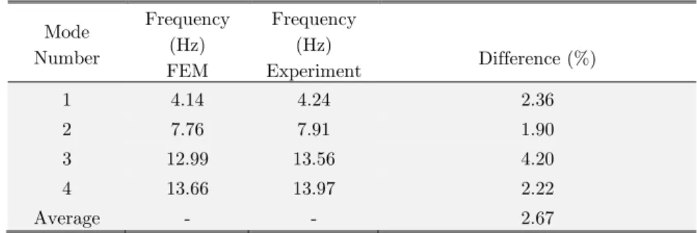
A modal analysis is performed to obtain the main natural frequencies and corresponding mode shapes. The first four natural frequencies of the floor pan’s basic model are reported in Table 2.
Mode Number
Frequency (Hz) FEM
Frequency (Hz)
Experiment Difference (%)
1 4.14 4.24 2.36
2 7.76 7.91 1.90
3 12.99 13.56 4.20
4 13.66 13.97 2.22
Average - - 2.67
Table 2: First four natural frequencies of the floor pan’s basic model of NP01 project found by FEM and Experiment.
3.1 Experimental Results and Validation of the FE Model
First four natural frequencies of the floor panel found by the experiment are listed in Table 2. A comparison with the FEM results shows the maximum and average difference of 4.2% and 2.67% respectively. A good accordance between the frequency results is observed. But this comparison is not enough to make sure about consistency of the mode shapes found by experiment and FEM. Hence, the MAC criterion is used to compare the first four mode shapes. The MAC has been used in the literature as a Mode Shape Correlation Constant to quantify the accuracy of identified mode shapes Pastor et al (2012). For complex modes of vibration the MAC value is found by:
, (1)
Table 3 shows the CrossMAC matrix calculating the MAC between the test model and the FEM model. The values close to 1 show a good accordance between the mode shapes and the values close to one state that there is almost no accordance between the corresponding mode shapes. As it is obvious in the Table, the diagonal values are close to one and demonstrate the good accuracy of the simulation method.
Frequency 4.14 7.76 12.29 13.66
4.24 0.791 0.002 0.201 0.085
7.91 0.002 0.785 0.006 0.005
13.56 0.201 0.006 0.810 0.128
13.97 0.085 0.005 0.128 0.736
Table 3: CrossMAC matrix to compare consistency of the experimental and FEM mode shapes.
4 PARAMETRIC STUDY
4.1 Design of Experiment by Taguchi Method
In this section, four geometrical parameters are considered as the design variables affecting two output functions: first natural frequency and total mass of the floor pan. These design variables are show in Figure 4. Based on design and production restrictions, the upper and lower bound for variations of the design variables are supposed as follows:
. mm . mm
mm mm
mm mm
mm mm
(2)
where t is the thickness of the panel and w, l and d are the width, length and depth of the panel’s embosses. The higher the number of levels, the lower effects of nonlinearity error in the parametric study becomes Ranjit et al (2001). However, four levels of variations are considered for each variable based on time and financial resources including t (0.65, 0.8, 0.9, and 1.2), w (20, 30, 40, and 48), l
(80, 103, 143, and 173), and d (2, 5, 10, and 15). Values of the four variables corresponding to each level are summarized in Table 4.
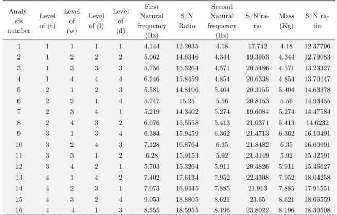
The total number of possible combinations of these variables according to number of levels and variables is equal to 256. In Taguchi method two main parameters are needed to be specified. First is control factor or the vector of design variables; another is the noise factor that denotes all factors that cause variation. Taguchi proposed orthogonal arrays to acquire the attribute data and to analyze the performance measure of the data to decide the optimal process parameters Senthil Kumar [14]. In this study, orthogonal array is employed. This array is suitable for the cases with four design variables and four levels for each design variable Ranjit et al (2001). The total number of experiments is 16 and the corresponding configuration of the experiments is shown in Table 5 (S/N ratio in this table is described in the next section).
Level Number t (mm) w (mm) l (mm) d (mm)
1 0.65 20 80 2
2 0.8 30 103 5
3 0.9 40 143 10
4 1.2 48 173 15
Table 4: Designated levels of the design variables.
Analy-sis number Level of (t) Level of (w) Level of (l) Level of (d) First Natural frequency (Hz) S/N Ratio Second Natural frequency (Hz) S/N ra-tio Mass (Kg) S/N ra-tio
1 1 1 1 1 4.144 12.2035 4.18 17.742 4.18 12.37796
2 1 2 2 2 5.062 14.6346 4.344 19.3953 4.344 12.79083
3 1 3 3 3 5.756 15.3264 4.571 20.5486 4.571 13.23327
4 1 4 4 4 6.246 15.8459 4.854 20.6338 4.854 13.70147
5 2 1 2 3 5.581 14.8106 5.404 20.3155 5.404 14.63378
6 2 2 1 4 5.747 15.25 5.56 20.8153 5.56 14.93455
7 2 3 4 1 5.219 14.3402 5.274 19.6084 5.274 14.47584
8 2 4 3 2 6.076 15.5558 5.413 21.0371 5.413 14.6232
9 3 1 3 4 6.384 15.9459 6.362 21.4713 6.362 16.10491
10 3 2 4 3 7.128 16.8764 6.35 21.8482 6.35 16.00991
11 3 3 1 2 6.28 15.9153 5.92 21.4149 5.92 15.42591
12 3 4 2 1 5.703 15.3264 5.911 20.4826 5.911 15.46627
13 4 1 4 2 7.402 17.6134 7.952 22.4308 7.952 18.04258
14 4 2 3 1 7.073 16.9445 7.885 21.913 7.885 17.91551
15 4 3 2 4 9.053 18.8805 8.621 23.65 8.621 18.66559
16 4 4 1 3 8.555 18.5955 8.196 23.8022 8.196 18.30508
Table 5: Modal results and S/N ratio analysis of the set of experiments proposed by Taguchi orthogonal array.
4.2 S/N ratio analysis
S/N ratio is an index which describes the signals to noise ratio in the Taguchi method. Signal and noise refer to mean (desirable) and standard deviation (undesirable) values of the output respectively. In reality, the target functions will be never fixed in a desired value. Hence, there are always fluctu-ations around the desired (mean) value which depend on external factors such as human errors and temperature effects; these uncontrollable factors are named as noise factors. The S/N ratio character-istics are classified into three categories based on the final decision on the performance:
Case 1: “Smaller is the better”
This case is valid when minimizing the output function is desired.
Case 2: “Nominal is the best”
This case is valid when the nominal or target value and variation about that value are minimized.
log ⋯
∑
(4)
Case 3: “Larger is the better”
This case is valid when maximizing the output function is desired.
log / (5)
In the above equations, N represents the number of repetition of each experiment and denotes the objective function. In the present study, the natural frequency of the floor pan is desired to make maximized and the total mass of the panel is supposed to make minimized. Therefore, the third case is suitable for maximizing frequency and the first case is desired to minimize the total mass of the panel. S/N ratio analysis results are presented in Table 5. Moreover, the graphical figures correspond-ing to S/N ratios of the first and second natural frequency and total mass with respect to the four design variables are depicted in Figures 5-7. Clearly, higher S/N ratios have led to the higher natural frequencies and higher weights. A big conflict is observed between the objective functions. First, let’s consider three separate cases:
Case I: If the first natural frequency is considered as a single objective function in this study, among the 16 cases of experiment, the last case has better results due to the higher natural frequency and S/N ratio. Table 6 shows the S/N ratio corresponding to each design variable in different levels. Based on this table and Figure 5 as well, the highest value of S/N ratio among all of the design variables is related to the fourth level. Therefore, the best combination of the design variables leading to the highest value of first natural frequency is predicted to be . According to Figure 5, thickness (t) with the sharpest slope is the most significant factor which affects the natural frequency. Secondly, the depth (d) is more important than the two other variables. The other fact observed in this figure is that variations of depth (d) will not have any significant effects on the natural frequency after the third level of depth.
the most significant factor which affects the natural frequency. Secondly, the depth (d) is more im-portant than the two other variables.
Case III: If the total mass of the panel is considered as a single objective function in this study, among the 16 cases of experiment, the first case (base model) has better results due to the lower mass and S/N ratio based on the results shown in Table 8. On the contrary, the last case has led to the worst results. According to Figure 7 and Table 8, S/N ratio analysis shows that thickness (t) and depth (d) are the most effecting parameters on the mass of the panel. But this effect is in the opposite way compared to the natural frequency; meaning that due to the mass growth, it is not desired to increase the thickness and depth of the emboss.
According to this conclusion, a big conflict is apparent between the first and second natural frequency and the total mass of the floor pan. In this situation, a good solution is using MCDM methods to find the best combination of the design variables leading to the trade-off values of the objective functions. An MCDM investigation is carried out in Section 5.
Level
Number t (mm) w (mm) l (mm) d (mm)
1 19.58 20.49 20.49 19.93
2 20.44 20.99 20.96 21.07
3 21.3 21.3 21.24 21.63
4 22.95 21.49 21.13 21.64
Rank 1 3 4 2
Table 6: S/N ratio response of the first natural frequency in different levels of control parameters.
Level
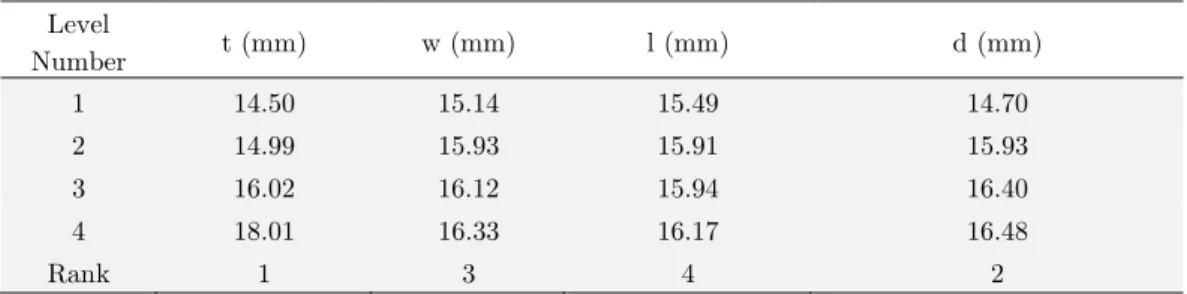
Number t (mm) w (mm) l (mm) d (mm)
1 14.50 15.14 15.49 14.70
2 14.99 15.93 15.91 15.93
3 16.02 16.12 15.94 16.40
4 18.01 16.33 16.17 16.48
Rank 1 3 4 2
Table 7: S/N ratio response of the second natural frequency in different levels of control parameters.
Level
Number t (mm) w (mm) l (mm) d (mm)
1 13.03 15.29 15.26 15.06
2 14.67 15.41 15.39 15.22
3 15.75 15.45 15.47 15.55
4 18.23 15.52 15.56 15.85
Rank 1 4 3 2
Figure 5: Signal to noise ratio graphs of the first natural frequency with respect to the four design variables in four different levels is shown in four sub-figures respectively.
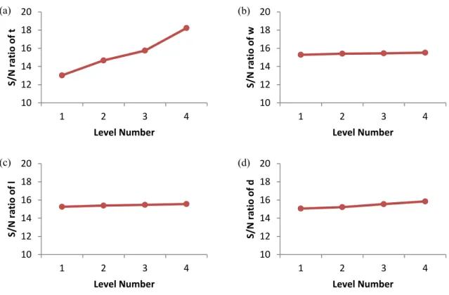
Figure 6: Signal to noise ratio graphs of the second natural frequency with respect to the four
design variables in four different levels is shown in four sub-figures respectively.
S/N ratio respet
to t
Le el Num er S/N ratio respet
to
Le el Num er
(b)
S/N ratio respet
to l
Le el Num er S/N ratio respet
to d
Le el Num er
(d)
S/N ratio respet
to t
Le el Num er S/N ratio respet
to
Le el Num er
(b)
S/N ratio respet
to l
Le el Num er S/N ratio respet
to d
Le el Num er
(d) (a)
(a) (c)
Figure 7: Signal to noise ratio graphs of the total mass with respect to the four design variables in four different levels is shown in four sub-figures respectively.
4.3 Analysis of Variance (ANOVA)
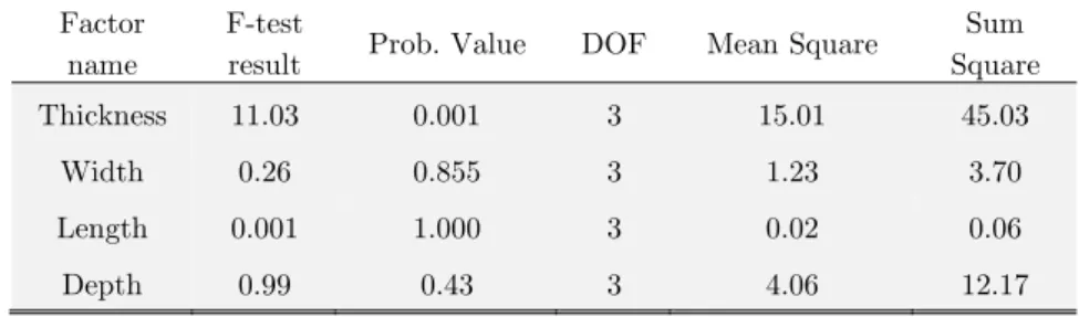
As verification for the S/N ratio results, ANOVA is performed to determine the effect of different design parameters on the output variables. Furthermore, contribution percentage of each control factor is determined from the results of this analysis. As seen, there is a statistical tool called an F test to see which design parameters has a significant effect on the quality characteristic. Usually, when F > 4, it means that the change of the design parameter has a significant effect on the quality characteristic Khalkhali. A, Noraei. H et al (2016). The higher the F-test result, the more contribution percentage in affecting the quality characteristics is expected. The results of this analysis are provided in Tables 9-11 for the first natural frequency, second natural frequency and mass respectively. As it is anticipated from Section 4.2 (S/N ratio analysis), the panel’s thickness is the most effective param-eter on the first and second natural frequency and mass with F-test values of 11.2, 11.03 and 142.14 respectively. Comparing to the first natural frequency, the total mass is more sensitive to the varia-tions of the panel’s thickness according to the F-test results. After that, the depth of emboss (d) has the highest response of F-test equal to 0.83, 0.99 and 0.09 for the first natural frequency, second natural frequency and mass respectively. This conclusion is completely approving the results found by the S/N ratio analysis. Additionally, the length of emboss (l) is the least important parameter in affecting the output value in this study.
S/N
ratio
of
t
Le el Num er
S/N
ratio
of
Le el Num er
S/N
ratio
of
l
Le el Num er
S/N
ratio
of
d
Le el Num er
(a)
(c) (d)
Factor name
F-test
result Prob. Value DOF Mean Square
Sum Square
Thickness 11.03 0.001 3 15.01 45.03
Width 0.26 0.855 3 1.23 3.70
Length 0.001 1.000 3 0.02 0.06
Depth 0.99 0.43 3 4.06 12.17
Table 9: Analysis of variance (ANOVA) of the first natural frequency with respect to different factors.
Factor name
F-test
result Prob. Value DOF Mean Square
Sum Square
Thickness 11.2 0.001 3 5.555 16.664
Width 0.28 0.838 3 0.5 1.49
Length 0.05 0.986 3 0.09 0.26
Depth 0.83 0.502 3 0.3 3.91
Table 10: Analysis of variance (ANOVA) of the second natural frequency with respect to different factors.
Factor name
F-test
result Prob. Value DOF Mean Square
Sum Square
Thickness 142.14 0.0001 3 9.76 29.29
Width 0.01 0.999 3 0.01 0.04
Length 0.01 0.999 3 0.01 0.04
Depth 0.09 0.962 3 2.45 0.69
Table 11: Analysis of variance (ANOVA) of the total mass with respect to different factors.
4.4 Numerical Validation
method and S/N ratio analysis are the optimum designs of the floor pan considering the first natural frequency and the second natural frequency separately as the single objective functions.
Strategy
St1 1 1 1
St2 2 2 1
1 1 2
Table 12: Geometrical configuration and output values of and case.
5 MULTI-CRITERIA DECISION MAKING
In this section, a new method is developed to find the trade-off design considering three objective functions, including the first natural frequency, the second natural frequency and the total mass. These quantities are selected to be optimized based on target cascading plan of the platform project to reduce the mass and improve the NVH characteristics of the panel. First, using Taguchi array a sixteen-sized set of experiments is defined as previously explained in Section 4. Now, a multi-criteria decision making (MCDM) method is needed to choose the trade-off design, among the present cases. Different strategies may be employed by engineers in MCDM problems based on the importance priorities that they previously designated to different attributes. Three different strategies are declared in Table 13 in case of choosing a trade-off design for the floor pan of a B-segment automotive body. The first strategy (St1) is used when there is no difference in importance of weight and stiffness attributes of the vehicle. The second and third strategies (St2 and St3) are used when stiffening or mass reduction is two times more important than the other respectively. A weight-sensitive MCDM method is needed to cope with such a problem which the objectives have different weight factors. Two different weight-sensitive MCDM methods are introduced and employed to choose the trade-off design with different strategies.
t (mm) w
(mm) l (mm)
d (mm)
First Natural frequency (Hz)
Second Natural
Fre-quency (Hz) Mass (Kg)
1.2 48 173 15 9.63 15.93 8.96
1.2 48 143 15 9.57 16.11 8.83
Table 13: Strategy definition and corresponding weight factors. ( , , are the weight
coefficients corresponding to first and second natural frequencies and mass respectively).
5.1 Sum of Variations Compared to the Base Design (SVCB)
In the first step, non-dimensional variation of each objective function is calculated:
∆ , , ,
, (6)
where, , is the i-th objective function of the j-th case and , is the i-th objective function of the base case.
Subsequently, the weighted sum of non-dimensional variations of the objective functions is ob-tained as follows:
∑ ∆ , , for j=1 to m (7)
where, NNI is the Non-dimensional Net Improvement in the objective functions of the j-th case com-pared to the base case, n is the number of objective functions, is the weight of i-th objective function, m is the number of design alternatives (cases) and k applies the effect of minimizing or maximizing the i-th objective function to the Equation 6, which is found using the following relation:
(8)
This method which is named as “Sum of Variations Compared to the Base Design (SVCB)” is set up to solve the current MCDM problem and is applicable to all of the weighted MCDM problems where a base design is supposed to be improved.
5.2 The Technique for Order of Preference by Similarity to Ideal Solution (TOPSIS)
TOPSIS is a conventional method used in this study to validate operation of the new developed MCDM method (SVCB). The objective of TOPSIS is to determine the best compromise solution based on the distance from the positive, (S+), and negative, (S-), ideal solutions according to the weights appointed for every criterion. The best solution is the closest one to the positive ideal solution and the farthest one from the negative ideal solution. This method is widely used in both engineering and non-engineering MCDM problems. The governing equations and the procedure of this method are present in the prior works Khalkhali et al (2014).
5.3 Results and Discussion
SVCB sorting of the Taguchi 16 cases is demonstrated in Table 14. Considering St1 or St2 as the current strategy, the fifteenth case is elected. Comparing the results of St1 with the base case, 119% improvement in the first natural frequency, 97% improvement in the second natural frequency and 106% deteriorating in the mass is observed. Totally, a non-dimensional net improvement (NNI) of 110% is observed in the three objective functions. An analogous conclusion is derived considering St2 as the current strategy. But NNI in this case is 327% due to the higher effect of natural frequency enhancements. If mass reduction is an important attribute in the automotive design, the third strategy St3 is suitable to be employed.
and second natural frequencies respectively, whereas a 32% unfavorable enhancement in the floor pan’s mass is also observed. Totally, the value of NNI is 58.6% compared to the base design.
Case
Number St1 St2 St3
TOPSIS SVCB TOPSIS SVCB TOPSIS SVCB
H Rank NNI Rank H Rank NNI Rank H Rank NNI Rank
1 (Base) 0.339 16 0 16 0.204 16 0 16 0.506 10 0 12
2 0.480 10 0.380 13 0.381 14 0.798 14 0.602 3 0.340 4
3 0.538 5 0.663 5 0.462 10 1.419 10 0.633 2 0.569 2
4 0.566 4 0.747 4 0.508 7 1.656 7 0.637 1 0.586 1
5 0.457 13 0.405 12 0.402 12 1.103 12 0.524 8 0.112 9
6 0.473 11 0.467 10 0.429 11 1.263 11 0.528 7 0.137 7
7 0.405 15 0.224 15 0.333 15 0.710 15 0.493 12
-0.038 13
8 0.533 6 0.637 6 0.495 8 1.569 9 0.581 4 0.342 3
9 0.492 9 0.539 9 0.488 9 1.600 8 0.496 11 0.017 11
10 0.580 3 0.811 3 0.594 3 2.140 3 0.563 5 0.291 5
11 0.529 7 0.632 7 0.513 6 1.680 6 0.549 6 0.215 6
12 0.433 14 0.319 14 0.397 13 1.052 13 0.478 14
-0.095 14
13 0.511 8 0.582 8 0.585 4 2.067 4 0.420 15
-0.320 15
14 0.466 12 0.445 11 0.528 5 1.776 5 0.390 16
-0.441 16
15 0.659 2 1.103 1 0.793 1 3.269 1 0.492 13 0.041 10
16 0.664 1 1.092 2 0.779 2 3.145 2 0.520 9 0.131 8
Table 14: TOPSIS and SVCB results and ranking for three different strategies.
Figure 8: The output domain, First natural frequency with respect to total mass of the panel.
Figure 9: The output domain, First natural frequency with respect to second natural frequency of the panel.
Figure 10: The output domain, second natural frequency with respect to total mass of the panel.
, , , , , , ,
Mass of the panel Kg
Fist
Natual Feuency Hz
, , , , , , ,
Second Natu al F e uency Hz
Fist
Natual Feuency Hz
Mass of the panel Kg
Second Natual Feuency Hz
St1, St2
St3
St1, St2
St3
St1, St2
(a)
1st mode: 4.14 Hz 2st mode: 7.76 Hz
3st mode: 12.99 Hz 4st mode: 13.66 Hz
(b)
1st mode: 6.25 Hz 2st mode: 10.84 Hz
3st mode: 15.31 Hz 4st mode: 18.76 Hz
(c)
1st mode: 9.05 Hz 2st mode: 15.32 Hz
3st mode: 23.01 Hz 4st mode: 29.93 Hz
Figure 11: Comparison of first four natural mode shapes of (a) the base case and the trade-off design introduced
The TOPSIS ranking of all cases with three different strategies are also shown in Table 14. A very good accordance between the results found by SVCB and TOPSIS is clearly observed. Therefore, the present method (SVCB) is trustable and has the following advantages over TOPSIS:
1-SVCB has a simpler and shorter procedure compared to TOPSIS
We face to a more complicated procedure in TOPSIS compared to SVCB. The first step in both methods is similar. Calculation of the non-dimensional variation for each alternative in SVCB and according to Khalkhali et al (2014), calculation of the normalized rating ̃ for each alternative in TOPSIS. However, this procedure is shorter and simpler in SVCB; because a division (SVCB) takes shorter time compared to a division along with calculation of square root of sum of squares (TOPSIS). The next steps are different in the two methods. In TOPSIS, first two parameters and must be calculated and then, two distances (the distance from best and worst virtual designs) are found using square root of sum of squares. But the next step in SVCB is much shorter and simpler; NNI is calculated using summation of a limited number of products.
2-In SVCB, it is possible to make a clear comparison between the trade-off design and the base case, based on negative or positive values of NNI.
In TOPSIS, no base case is defined. Instead, a virtual best and a virtual worst point are considered. Therefore, in TOPSIS the best alternative is the design which has the minimum relative closeness to the virtual best point. This gives no sense about being the results better or worse compared to a base case. In SVCB, the negative, zero or positive value of NNI clearly gives information about being worse, equal or better than the base case.
It should be noted that requiring a base design is not a limitation for SVCB. If a base case is not available, an arbitrary design case could be chosen as the base case among all of the present cases. In this situation, the trade-off design corresponds to the highest positive value of NNI.
6 CONCLUSIONS
tive functions. The thickness of panel is found to be the most effective parameter on the both objec-tives simultaneously. Then, an MCDM method was developed to consider the effects of first natural frequency, second natural frequency and mass at the same time. Three strategies were introduced based on the importance of different parameters deciding according to the automotive design attrib-utes. Considering these three strategies, trade-off ranking was reported using the new developed MCDM method (SVCB) and the conventional method (TOPSIS). A very good accordance was ob-served between the rankings found by two methods. Using this newly developed MCDM model, NNI of the trade-off design associated with St1 and St2 was reported to be 110% showing a good improve-ment in total behavior of the floor pan.
References
Abolfazl Khalkhali, Sharif Khakshournia, Nader Narimanzadeh. (2014). A hybrid method of FEM, modified NSGAII and TOPSIS for structural optimization of sandwich panels with corrugated core. Journal of Sandwich Structures and Materials .
Abolfazl Khalkhali, Sharif Khakshournia, Parvaneh Saberi. (2016). Optimal design of functionally graded PmPV/CNT nanocomposite cylindrical tube for purpose of torque transmission. Journal of Central South University , 23 (2), 362-9.
B. Chaturved, D. Rana and M. Ravindran. (2010). Correlation of vehicle dynamics & NVH performance with body static & dynamic stiffness through CAE and experimental analysis. SAE World Congress and Exhibition , 1-8. Eun Suk Suh, Olivier de Weck, Yong Kim, David Chang. (2007). Flexible platform component design under uncer-tainty. Journal of Intelligent Manufacturing , 18, 115-26.
Ewins, D. J. (1984). Modal testing: theory and practice (Vol. 15). Letchworth: Research studies press.
Guangyong Sun, Jiang Fang, Xuanyi Tian, Guangyo Li, Qing Li. (2015). Discrete robust optimization algorithm based on Taguchi method for structural crashworthiness design. Expert Systems with Applications , 42, 4482-92.
Guangyong,S. Jiang,F. Xuanyi,T. Guangyo,L. Qing,L. (2015). Discrete robust optimization algorithm based on Taguchi method for structural crashworthiness design. Expert Systems with Applications , 42, 4482-92.
Hari Krishnan. (2011). Establishing correlation between torsional and lateral stiffness parameters of BIW and vehicle handling performance. SAR International Journal of Passenger Cars , 4, 22-31.
Khalkhali, A., Noraie, H., & Sarmadi, M. (2016). Sensitivity analysis and optimization of hot-stamping process of automotive components using analysis of variance and Taguchi technique. Proceedings of the Institution of Mechanical Engineers, Part E: Journal of Process Mechanical Engineering, 0954408916633491.
Khalkhali,A. Khakshournia,S. Saberi,P. (2016). Optimal design of functionally graded PmPV/CNT nanocomposite cylindrical tube for purpose of torque transmission. Journal of Central South University , 23 (2), 362-9.
Khalkhali,A. Khakshournia,Sh. Narimanzadeh,N. (2014). A hybrid method of FEM, modified NSGAII and TOPSIS for structural optimization of sandwich panels with corrugated core. Journal of Sandwich Structures and Materials . Krishnan, H. (2011). Establishing correlation between torsional and lateral stiffness parameters of BIW and vehicle handling performance. SAR International Journal of Passenger Cars , 4, 22-31.
Kumar,P. Singh D. Patel S.B. Parsad. (2016). Optimization of process parameters during vibratory welding technique usin Taguchi's analysis. Perspectives in Science , Accepted Manuscript.
LMS theory and background (2000), LMS International 2000.
Mathan Kumar, N. S. (2016). Aerospace application on Al 2618 with reinforced - Si3N4, AIN and ZrB2 in-situ com-posites. Journal of Alloys and Compounds , 672, 238-50.
Mohan Kumar G R, Dr. Maruthi B H, Chandru B T, Manoranjan S N. (2015). Vibration analysis of automotive car floor using FEM and FFT analyzer. International Journal for Technological Research in Engineering , 2 (11), 2891-96. Mohan Kumar, G.R., Maruthi, B.H. Chandru,B.T. Manoranjan,S.N. (2015). Vibration analysis of automotive car floor using FEM and FFT analyzer. International Journal for Technological Research in Engineering , 2 (11), 2891-96. N. Mathan Kumar, S. S. (2016). Aerospace application on Al 2618 with reinforced - Si3N4, AIN and ZrB2 in-situ composites. Journal of Alloys and Compounds , 672, 238-50.
P. Senthil Kumar, R. Kalidas, K. Sivakumar, E. Hariharan, B. Gautham, R. Ethiraj. (2013). Application of Taguchi method for optimizating passenger- friendly vehicle suspension system. International Journal of Latest Trends in En-gineering and Technology , 2 (1).
Palmonella, Matteo, Michael l. Friswell, John E. and Arthur W, Lees. (2005). Finite element models of spot welds in structural dynamics: review and updating. Computers & Structures , 83 (8), 648-61.
Parvin Kumar, Singh D. Patel S.B. Parsad. (2016). Optimization of process parameters during vibratory welding technique usin Taguchi's analysis. Perspectives in Science , Accepted Manuscript.
Pastor, M., Binda, M., & Harčarik, T. (2012). Modal assurance criterion. Procedia Engineering, 48, 543-548. Ranjit, K. (2001). Roy. Design of experiments using the Taguchi approach. John Willey & Sons Inc., New York. Shin, Jaeho, Neng Yue and Costin D. Untaroiu. (2012). A finite element model of the foot and ankle for automotive impact applications. Annals of Biomedical Engineering , 40 (12), 2519-31.
Sobieszczansk,S. Jaroslaw, Srinivas,K.Yang, R. (2001). Optimization of car body under constraints of noise, vibration and harshness (NVH) and crash. Structural and Multidisciplinary Optimization , 22 (4), 295-306.
Sobieszczanski-Sobieski, Jaroslaw, Srinivas Kodiyalam, R.Y. Yang. (2001). Optimization of car body under constraints of noise, vibration and harshness (NVH) and crash. Structural and Multidisciplinary Optimization , 22 (4), 295-306. Steve Kline, J. (March 2016). Automotive Production Growth Strong. Plastics Technology .
Steve Kline, J. (March 2016). Automotive Production Growth Strong. Plastics Technology .
Steven Tebby, Ahmad Barari and Ebrahim Esmailzadeh. (2012). Analysis and optimization of automotive's structure's bending stiffness using beam elements. ASME, 14th International Conference on Advanced Vehicle Technologies , 6, 12-15.
Suh,E. Weck,O. Kim,Y. Chang,D. (2007). Flexible platform component design under uncertainty. Journal of Intelligent Manufacturing , 18, 115-26.
Taguchi G., Konishi S. (1987). Taguchi methods, orthogonal arrays and linear graphs, tools for quality. Ammerican Supplier Institute , 8-35.
The global automotive market. (2014). Economic Outlook , 1210, 1-20.
Wang Mingqi, Jin Guodong. (1997). The application of Taguchi method to the stiffness improvement of a double- decker structure. International Journal of Materials and Product Technology (4-6).