Repositório ISCTE-IUL
Deposited in Repositório ISCTE-IUL:
2019-03-27
Deposited version:
Post-print
Peer-review status of attached file:
Peer-reviewed
Citation for published item:
Moro, S., Cortez, P. & Rita, P. (2014). A data-driven approach to predict the success of bank telemarketing. Decision Support Systems. 62, 22-31
Further information on publisher's website:
10.1016/j.dss.2014.03.001
Publisher's copyright statement:
This is the peer reviewed version of the following article: Moro, S., Cortez, P. & Rita, P. (2014). A data-driven approach to predict the success of bank telemarketing. Decision Support Systems. 62, 22-31, which has been published in final form at https://dx.doi.org/10.1016/j.dss.2014.03.001. This article may be used for non-commercial purposes in accordance with the Publisher's Terms and Conditions for self-archiving.
Use policy
Creative Commons CC BY 4.0
The full-text may be used and/or reproduced, and given to third parties in any format or medium, without prior permission or charge, for personal research or study, educational, or not-for-profit purposes provided that:
• a full bibliographic reference is made to the original source • a link is made to the metadata record in the Repository • the full-text is not changed in any way
The full-text must not be sold in any format or medium without the formal permission of the copyright holders.
A Data-Driven Approach to Predict the
Success of Bank Telemarketing
S´
ergio Moro
a,∗ Paulo Cortez
bPaulo Rita
aaISCTE - University Institute of Lisbon, 1649-026 Lisboa, Portugal bALGORITMI Research Centre, Univ. of Minho, 4800-058 Guimar˜aes, Portugal
Abstract
We propose a data mining (DM) approach to predict the success of telemarketing calls for selling bank long-term deposits. A Portuguese retail bank was addressed, with data collected from 2008 to 2013, thus including the effects of the recent finan-cial crisis. We analyzed a large set of 150 features related with bank client, product and social-economic attributes. A semi-automatic feature selection was explored in the modeling phase, performed with the data prior to July 2012 and that allowed to select a reduced set of 22 features. We also compared four DM models: logistic regression, decision trees (DT), neural network (NN) and support vector machine. Using two metrics, area of the receiver operating characteristic curve (AUC) and area of the LIFT cumulative curve (ALIFT), the four models were tested on an eval-uation phase, using the most recent data (after July 2012) and a rolling windows scheme. The NN presented the best results (AUC=0.8 and ALIFT=0.7), allowing to reach 79% of the subscribers by selecting the half better classified clients. Also, two knowledge extraction methods, a sensitivity analysis and a DT, were applied to the NN model and revealed several key attributes (e.g., Euribor rate, direction of the call and bank agent experience). Such knowledge extraction confirmed the obtained model as credible and valuable for telemarketing campaign managers.
Key words: Bank deposits, Telemarketing, Savings, Classification, Neural Networks, Variable Selection
1 Introduction
Marketing selling campaigns constitute a typical strategy to enhance busi-ness. Companies use direct marketing when targeting segments of customers by contacting them to meet a specific goal. Centralizing customer remote in-teractions in a contact center eases operational management of campaigns. Such centers allow communicating with customers through various channels, telephone (fixed-line or mobile) being one of the most widely used. Market-ing operationalized through a contact center is called telemarketMarket-ing due to the remoteness characteristic [16]. Contacts can be divided in inbound and outbound, depending on which side triggered the contact (client or contact center), with each case posing different challenges (e.g., outbound calls are often considered more intrusive). Technology enables rethinking marketing by focusing on maximizing customer lifetime value through the evaluation of available information and customer metrics, thus allowing to build longer and tighter relations in alignment with business demand [28]. Also, it should be stressed that the task of selecting the best set of clients, i.e., that are more likely to subscribe a product, is considered NP-hard in [31].
Decision support systems (DSS) use information technology to support man-agerial decision making. There are several DSS sub-fields, such as personal and intelligent DSS. Personal DSS are related with small-scale systems that
support a decision task of one manager, while intelligent DSS use artificial intelligence techniques to support decisions [1]. Another related DSS concept is Business Intelligence (BI), which is an umbrella term that includes informa-tion technologies, such as data warehouses and data mining (DM), to support decision making using business data [32]. DM can play a key role in personal and intelligent DSS, allowing the semi-automatic extraction of explanatory and predictive knowledge from raw data [34]. In particular, classification is the most common DM task [10] and the goal is to build a data-driven model that learns an unknown underlying function that maps several input variables, which characterize an item (e.g., bank client), with one labeled output target (e.g., type of bank deposit sell: “failure” or “success”).
There are several classification models, such as the classical Logistic Regres-sion (LR), deciRegres-sion trees (DT) and the more recent neural networks (NN) and support vector machines (SVM) [13]. LR and DT have the advantage of fit-ting models that tend to be easily understood by humans, while also providing good predictions in classification tasks. NN and SVM are more flexible (i.e., no a priori restriction is imposed) when compared with classical statistical mod-eling (e.g., LR) or even DT, presenting learning capabilities that range from linear to complex nonlinear mappings. Due to such flexibility, NN and SVM tend to provide accurate predictions, but the obtained models are difficult to be understood by humans. However, these “black box” models can be opened by using a sensitivity analysis, which allows to measure the importance and effect of particular input in the model output response [7]. When comparing DT, NN and SVM, several studies have shown different classification perfor-mances. For instance, SVM provided better results in [6][8], comparable NN and SVM performances were obtained in [5], while DT outperformed NN and
SVM in [24]. These differences in performance emphasize the impact of the problem context and provide a strong reason to test several techniques when addressing a problem before choosing one of them [9].
DSS and BI have been applied to banking in numerous domains, such as credit pricing [25]. However, the research is rather scarce in terms of the specific area of banking client targeting. For instance, [17] described the potential useful-ness of DM techniques in marketing within Hong-Kong banking sector but no actual data-driven model was tested. The research of [19] identified clients for targeting at a major bank using pseudo-social networks based on relations (money transfers between stakeholders). Their approach offers an interesting alternative to traditional usage of business characteristics for modeling.
In previous work [23], we have explored data-driven models for modeling bank telemarketing success. Yet, we only achieved good models when using at-tributes that are only known on call execution, such as call duration. Thus, while providing interesting information for campaign managers, such models cannot be used for prediction. In what is more closely related with our ap-proach, [15] analyzed how a mass media (e.g., radio and television) marketing campaign could affect the buying of a new bank product. The data was col-lected from an Iran bank, with a total of 22427 customers related with a six month period, from January to July of 2006, when the mass media campaign was conducted. It was assumed that all customers who bought the product (7%) were influenced by the marketing campaign. Historical data allowed the extraction of a total of 85 input attributes related with recency, frequency and monetary features and the age of the client. A binary classification task was modeled using a SVM algorithm that was fed with 26 attributes (after a fea-ture selection step), using 2/3 randomly selected customers for training and
1/3 for testing. The classification accuracy achieved was 81% and through a Lift analysis [3], such model could select 79% of the positive responders with just 40% of the customers. While these results are interesting, a robust validation was not conducted. Only one holdout run (train/test split) was considered. Also, such random split does not reflect the temporal dimension that a real prediction system would have to follow, i.e., using past patterns to fit the model in order to issue predictions for future client contacts.
In this paper, we propose a personal and intelligent DSS that can automati-cally predict the result of a phone call to sell long term deposits by using a DM approach. Such DSS is valuable to assist managers in prioritizing and se-lecting the next customers to be contacted during bank marketing campaigns. For instance, by using a Lift analysis that analyzes the probability of success and leaves to managers only the decision on how many customers to contact. As a consequence, the time and costs of such campaigns would be reduced. Also, by performing fewer and more effective phone calls, client stress and intrusiveness would be diminished. The main contributions of this work are:
• We focus on feature engineering, which is a key aspect in DM [10], and pro-pose generic social and economic indicators in addition to the more com-monly used bank client and product attributes, in a total of 150 analyzed features. In the modeling phase, a semi-automated process (based on busi-ness knowledge and a forward method) allowed to reduce the original set to 22 relevant features that are used by the DM models.
• We analyze a recent and large dataset (52944 records) from a Portuguese bank. The data were collected from 2008 to 2013, thus including the effects of the global financial crisis that peaked in 2008.
rolling windows evaluation and two classification metrics. We also show how the best model (NN) could benefit the bank telemarketing business.
The paper is organized as follows: Section 2 presents the bank data and DM approach; Section 3 describes the experiments conducted and analyzes the obtained results; finally, conclusions are drawn in Section 4.
2 Materials and Methods
2.1 Bank telemarketing data
This research focus on targeting through telemarketing phone calls to sell long-term deposits. Within a campaign, the human agents execute phone calls to a list of clients to sell the deposit (outbound) or, if meanwhile the client calls the contact-center for any other reason, he is asked to subscribe the deposit (inbound). Thus, the result is a binary unsuccessful or successful contact.
This study considers real data collected from a Portuguese retail bank, from May 2008 to June 2013, in total of 52944 phone contacts. The dataset is unbalanced, as only 6557 (12.38%) records are related with successes. For evaluation purposes, a time ordered split was initially performed, where the records were divided into training (four years) and test data (one year). The training data is used for feature and model selection and includes all contacts executed up to June 2012, in a total of 51651 examples. The test data is used for measuring the prediction capabilities of the selected data-driven model, including the most recent 1293 contacts, from July 2012 to June 2013.
“suc-cess”}), and candidate input features. These include telemarketing attributes (e.g., call direction), product details (e.g., interest rate offered) and client in-formation (e.g., age). These records were enriched with social and economic influence features (e.g., unemployment variation rate), by gathering external
data from the central bank of the Portuguese Republic statistical web site1.
The merging of the two data sources led to a large set of potentially useful features, with a total of 150 attributes, which are scrutinized in Section 2.4.
2.2 Data mining models
In this work, we test four binary classification DM models, as implemented in the rminer package of the R tool [5]: logistic regression (LR), decision trees (DT), neural network (NN) and support vector machine (SVM).
The LR is a popular choice (e.g., in credit scoring) that operates a smooth nonlinear logistic transformation over a multiple regression model and allows
the estimation of class probabilities [33]: p(c|xk) = 1+exp(w 1
0+PMi=1wixk,i)
, where
p(c|x) denotes the probability of class c given the k-th input example xk =
(xk,1, ..., xk,M) with M features and wi denotes a weight factor, adjusted by the
learning algorithm. Due to the additive linear combination of its independent variables (x), the model is easy to interpret. Yet, the model is quite rigid and cannot model adequately complex nonlinear relationships.
The DT is a branching structure that represents a set of rules, distinguishing values in a hierarchical form [2]. This representation can translated into a set of IF-THEN rules, which are easy to understand by humans.
The multilayer perceptron is the most popular NN architecture [14]. We adopt a multilayer perceptron with one hidden layer of H hidden nodes and one output node. The H hyperparameter sets the model learning complexity. A NN with a value of H = 0 is equivalent to the LR model, while a high H value
allows the NN to learn complex nonlinear relationships. For a given input xk
the state of the i-th neuron (si) is computed by: si = f (wi,0+Pj∈Piwi,j× sj),
where Pi represents the set of nodes reaching node i; f is the logistic function;
wi,j denotes the weight of the connection between nodes j and i; and s1 = xk,1,
. . ., sM = xk,M. Given that the logistic function is used, the output node
automatically produces a probability estimate (∈ [0, 1]). The NN final solution is dependent of the choice of starting weights. As suggested in [13], to solve this
issue, the rminer package uses an ensemble of Nr different trained networks
and outputs the average of the individual predictions [13].
The SVM classifier [4] transforms the input x ∈ <M space into a high
m-dimensional feature space by using a nonlinear mapping that depends on a kernel. Then, the SVM finds the best linear separating hyperplane, related to a set of support vector points, in the feature space. The rminer package adopts the popular Gaussian kernel [13], which presents less parameters than
other kernels (e.g., polynomial): K(x, x0) = exp(−γ||x − x0||2), γ > 0. The
probabilistic SVM output is given by [35]: f (xi) =Pmj=1yjαjK(xj, xi) + b and
p(i) = 1/(1 + exp(Af (xi) + B)), where m is the number of support vectors,
yi ∈ {−1, 1} is the output for a binary classification, b and αj are coefficients
of the model, and A and B are determined by solving a regularized maximum likelihood problem.
Before fitting the NN and SVM models, the input data is first standardized to a zero mean and one standard deviation [13]. For DT, rminer adopts the
default parameters of the rpart R package, which implements the popular CART algorithm [2] For the LR and NN learning, rminer uses the efficient BFGS algorithm [22], from the family of quasi-Newton methods, while SVM is trained using the sequential minimal optimization (SMO) [26]. The learning capabilities of NN and SVM are affected by the choice of their hyperparameters (H for NN; γ and C, a complex penalty parameter, for SVM). For setting these values, rminer uses grid search and heuristics [5].
Complex DM models, such as NN and SVM, often achieve accurate predictive performances. Yet, the increased complexity of NN and SVM makes the final data-driven model difficult to be understood by humans. To open these black-box models, there are two interesting possibilities, rule extraction and sensi-tivity analysis. Rule extraction often involves the use of a white-box method (e.g., decision tree) to learn the black-box responses [29]. The sensitivity anal-ysis procedure works by analyzing the responses of a model when a given input is varied through its domain [7]. By analyzing the sensitivity responses, it is possible to measure input relevance and average impact of a particular input in the model. The former can be shown visually using an input importance bar plot and the latter by plotting the Variable Effect Characteristic (VEC) curve. Opening the black-box allows to explaining how the model makes the decisions and improves the acceptance of prediction models by the domain experts, as shown in [20].
2.3 Evaluation
A class can be assigned from a probabilistic outcome by assigning a threshold
charac-teristic (ROC) curve shows the performance of a two class classifier across the range of possible threshold (D) values, plotting one minus the specificity (x-axis) versus the sensitivity (y-axis) [11]. The overall accuracy is given by
the area under the curve (AU C = R1
0 ROCdD), measuring the degree of
dis-crimination that can be obtained from a given model. AUC is a popular classi-fication metric [21] that presents advantages of being independent of the class frequency or specific false positive/negative costs. The ideal method should present an AUC of 1.0, while an AUC of 0.5 denotes a random classifier.
In the domain of marketing, the Lift analysis is popular for accessing the quality of targeting models [3]. Usually, the population is divided into deciles, under a decreasing order of their predictive probability for success. A useful Lift cumulative curve is obtained by plotting the population samples (ordered by the deciles, x-axis) versus the cumulative percentage of real responses cap-tured (y-axis). Similarly to the AUC metric, the ideal method should present an area under the LIFT (ALIFT) cumulative curve close to 1.0. A high ALIFT confirms that the predictive model concentrates responders in the top deciles, while a ALIFT of 0.5 corresponds to the performance of a random baseline.
Given that the training data includes a large number of contacts (51651), we adopt the popular and fast holdout method (with R distinct runs) for feature and model selection purposes. Under this holdout scheme, the training data is further divided into training and validation sets by using a random split with 2/3 and 1/3 of the contacts, respectively. The results are aggregated by the average of the R runs and a Mann-Whitney non-parametric test is used to check statistical significance at the 95% confidence level.
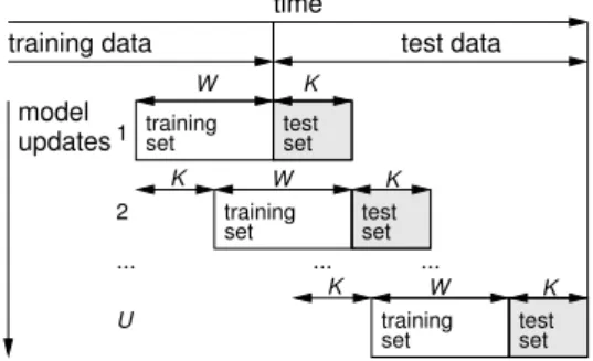
becomes available. Moreover, client propensity to subscribe a bank product may evolve through time (e.g., changes in the economic environment). Hence, for achieving a robust predictive evaluation we adopt the more realistic fixed-size (of length W ) rolling windows evaluation scheme that performs several model updates and discards oldest data [18]. Under this scheme, a training window of W consecutive contacts is used to fit the model and then we perform predictions related with the next K contacts. Next, we update (i.e., slide) the training window by replacing the oldest K contacts with K newest contacts (related with the previously predicted contacts but now we assume that the outcome result is known), in order to perform new K predictions, an so on. For a test set of length L, a total of number model updates (i.e., trainings) is U = L/K. Figure 1 exemplifies the rolling windows evaluation procedure.
K W K
training set testset 2
K W K
training set testset 1 trainingset settest
W K test data training data time ... ... ... U updates model
Fig. 1. Schematic of the adopted rolling windows evaluation procedure.
2.4 Feature selection
The large number (150) of potential useful features demanded a stricter choice of relevant attributes. Feature selection is often a key DM step, since it is useful to discard irrelevant inputs, leading to simpler data-driven models that are easier to interpret and that tend to provide better predictive performances [12]. In [34], it is argued that while automatic methods can be useful, the
best way is to perform a manual feature selection by using problem domain knowledge, i.e., by having a clear understanding of what the attributes actually mean. In this work, we use a semi-automatic approach for feature selection based on two steps that are described below.
In the first step, business intuitive knowledge was used to define a set of fourteen questions, which represent certain hypotheses that are tested. Each question (or factor of analysis) is defined in terms of a group of related at-tributes selected from the original set of 150 features by a bank campaign manager (domain expert). For instance, the question about the gender influ-ence (male/female) includes the three features, related with the gender of the banking agent, client and client-agent difference (0 – if same sex; 1 – else). Table 1 exhibits the analyzed factors and the number of attributes related with each factor, covering a total of 69 features (reduction of 46%).
In the second step, an automated selection approach is adopted, based an adapted forward selection method [12]. Given that standard forward selection is dependent on the sequence of features used and that the features related with a factor of analysis are highly related, we first apply a simple wrapper selection method that works with a DM fed with combinations of inputs taken from a single factor. The goal is to identify the most interesting factors and features attached to such factors. Using only training set data, several DM models are fit, by using: each individual feature related to a particular question (i.e., one input) to predict the contact result; and all features related with the same
question (e.g., 3 inputs for question #2 about gender influence). Let AU Cq
and AU Cq,i denote the AUC values, as measured on the validation set, for the
model fed with all inputs related with question q and only the i−th individual feature of question q. We assume that the business hypothesis is confirmed if
Table 1
Analyzed business questions for a successful contact result
Question (factor of analysis) Number of
features
1: Is offered rate relevant? 5
2: Is gender relevant? 3
3: Is agent experience relevant? 3
4: Are social status and stability relevant? 5
5: Is client-bank relationship relevant? 11
6: Are bank blocks (triggered to prevent certain operations) relevant? 6
7: Is phone call context relevant? 4
8: Are date and time conditions relevant? 3
9: Are bank profiling indicators relevant? 7
10: Are social and economic indicators relevant? 11
11: Are financial assets relevant? 3
12: Is residence district relevant? 1
13: Can age be related to products with longer term periods? 3 14: Are web page hits (for campaigns displayed in bank web sites) relevant? 4 Number of features after business knowledge selection 69 Number of features after first feature selection phase 22
at least one of the individually tested attributes achieves an AU Cq,i greater
than a threshold T1 and if the model will all question related features returns
an AU Cq greater than another threshold T2. When an hypothesis is confirmed,
only the m−th feature is selected if AU Cq,m > AU Cqor AU Cq−AU Cq,m < T3,
where AU Cq,m= max (AU Cq,i). Else, we rank the input relevance of the model
with all question related features in order to select the most relevant ones, such
that the sum of input importances is higher than a threshold T4.
Once a set of confirmed hypotheses and relevant features is achieved, a forward selection method is applied, working on a factor by factor step basis. A DM model that is fed with training set data using as inputs all relevant features of
the first confirmed factor and then AUC is computed over the validation set. Then, another DM model is trained with all previous inputs plus the relevant features of the next confirmed factor. If there is an increase in the AUC, then the current factor features are included in the next step DM model, else they are discarded. This procedure ends when all confirmed factors have been tested if they improve the predictive performance in terms of the AUC value.
3 Experiments and Results
3.1 Modeling
All experiments were performed using the rminer package and R tool [5] and conducted in a Linux server, with an Intel Xeon 5500 2.27GHz processor. Each DM model related with this section was executed using a total of R = 20 runs. For the feature selection, we adopted the NN model described in Section 2.2 as the base DM model, since preliminary experiments, using only training data, confirmed that NN provided the best AUC and ALIFT results when compared with other DM methods. Also, these preliminary experiments confirmed that SVM required much more computation when compared with NN, in an ex-pected result since SMO algorithm memory and processing requirements grow much more heavily with the size of the dataset when compared with BFGS algorithm used by the NN. At this stage, we set the number of hidden nodes using the heuristic H = round(M/2) (M is the number of inputs), which is also adopted by the WEKA tool [34] and tends to provide good classification
results [5]. The NN ensemble is composed of Nr = 7 distinct networks, each
Before executing the feature selection, we fixed the initial phase thresholds
to reasonable values: T1 = 0.60 and T2 = 0.65, two AUC values better than
the random baseline of 0.5 and such that T2 > T1; T3 = 0.01, the minimum
difference of AUC values; and T4 =60%, such that the sum of input
impor-tances accounts for at least 60% of the influence. Table 1 presents the eight confirmed hypothesis (question numbers in bold) and associated result of 22 relevant features, after applying the first feature selection phase. This proce-dure discarded 6 factors and 47 features, leading to a 32% reduction rate when compared with 69 features set by the business knowledge selection. Then, the forward selection phase was executed. Table 2 presents the respective AUC re-sults (column AUC, average of R = 20 runs) and full list of selected features. The second phase confirmed the relevance of all factors, given that each time a new factor was added, the DM model produced a higher AUC value. An additional experiment was conducted with the LR model, executing the same feature selection method and confirmed the same eight factors of analysis and leading to a similar reduced set (with 24 features). Yet, the NN model with 22 inputs got better AUC and ALIFT values when compared with LR, and thus such 22 inputs are adopted in the remaining of this paper.
After selecting the final set of input features, we compared the performance of the four DM models: LR, DT, NN, SVM. The comparison of SVM with NN was set under similar conditions, where the best hyperparameters (H and γ) were set by performing a grid search under the ranges H ∈ {0, 2, 6, 8, 10, 12} and
γ ∈ 2k : k ∈ {−15, −11.4, −7.8, −4.2, −0.6, 3}. The second SVM parameter
(which is less relevant) was fixed using the heuristic C = 3 proposed in for x standardized input data [5]. The rminer package applies this grid search by performing an internal holdout scheme over the training set, in order to select
Table 2
Final set of selected attributes
Factor Attributes Description AUC
1: interest rate
nat.avg.rate national monthly average of deposits interest rate 0.781 suited.rate most suited rate to the client according to bank
criteria
dif.best.rate.avg difference between best rate offered and the na-tional average
2: gender ag.sex sex of the agent (male/female) that made (out-bound) or answered (in(out-bound) the call
0.793
3: agent experience
ag.generic if generic agent, i.e. temporary hired, with less experience (yes/no)
0.799
ag.created number of days since the agent was created 5:
client-bank relationship
cli.house.loan if the client has a house loan contract (yes/no) 0.805 cli.affluent if is an affluent client (yes/no)
cli.indiv.credit if has an individual credit contract (yes/no) cli.salary.account if has a salary account (yes/no)
7: phone call context
call.dir call direction (inbound/outbound) 0.809 call.nr.schedules number of previously scheduled calls during the
same campaign
call.prev.durations duration of previously scheduled calls (in s) 8: date and
time
call.month month in which the call is made 0.810
9: bank profiling indicators
cli.sec.group security group bank classification 0.927 cli.agreggate if the client has aggregated products and services cli.profile generic client profile, considering assets and risk
10: social and economic indicators
emp.var.rate employment variation rate, with a quarterly fre-quency
0.929
cons.price.idx monthly average consumer price index cons.conf.idx monthly average consumer confidence index euribor3m daily three month Euribor rate
nr.employed quarterly average of the total number of employed citizens
the best hyperparameter (H or γ) that corresponds to the lowest AUC value measured on a subset of the training set, and then trains the best model with all training set data.
The obtained results for the modeling phase (using only training and validation set data) are shown on Table 3 in terms of the average (over R = 20 runs) of the AUC and ALIFT metrics (Section 2.3) computed on the validation set. The best result was achieved by the NN model, which outperformed LR (improvement of 3 pp), DT (improvement of 10 pp) and SVM (improvement of 4 and 3 pp) in both metrics and with statistical confidence (i.e., Mann-Whitney p-value<0.05). In the table, the selected NN and SVM hyperparameters are presented in brackets (median value shown for H and γ). It should be noted that the hidden node grid search strategy for NN did not improve the AUC value (0.929) when compared with the H = round(M/2) = 11 heuristic (used in Table 2). Nevertheless, given that a simpler model was selected (i.e., H = 6), we opt for such model in the remainder of this paper.
Table 3
Comparison of DM models for the modeling phase (bold denotes best value) Metric LR DT SVM (˜γ = 2−7.8, C = 3) NN ( ˜H = 6, Nr = 7)
AUC 0.900 0.833 0.891 0.929?
ALIFT 0.849 0.756 0.844 0.878?
? - Statistically significant under a pairwise comparison with SVM, LR and DT.
To attest the utility of the proposed feature selection approach, we compared it with two alternatives: no selection, which makes use of the all 150 features; and forward selection, which adopts the standard forward method. The latter alternative uses all 150 features as feature candidates. In the first iteration, it selects the feature that produces the highest AUC value, measured using the validation set (1/3 of the training data) when considering the average of
20 runs. Then, the selected feature is fixed and a second iteration is executed to select the second feature within the remaining 149 candidates and the obtained AUC is compared with the one obtained in previous iteration. This method proceeds with more iterations until there is no AUC improvement or if all features are selected. Table 4 compares the three feature selection methods in terms of number of features used by the model, time elapsed and performance metric (AUC). The obtained results confirm the usefulness of the proposed approach, which obtains the best AUC value. The proposed method uses lesser features (around a factor of 7) when compared with the full feature approach. Also, it is also much faster (around a factor of 5) when compared with the simple forward selection.
Table 4
Comparison of feature selection methods for the modeling phase using NN model (bold denotes best AUC)
Method #Features Time Elapsed (in s) AUC Metric
no selection 150 3223 0.832
forward selection 7 97975 0.896
proposed 22 18651∗ 0.929
∗ - includes interview with domain expert (5400s) for Table 1 definition.
3.2 Predictive knowledge and potential impact
The best model from previous section (NN fed with 22 features from Table 2,
with H = 6 and Nr = 7) was tested for its predictive capabilities under
a more realistic and robust evaluation scheme. Such scheme is based on a rolling windows evaluation (Section 2.3) over the test data, with L = 1293 contacts from the most recent year. Taking into account the computational effort required, the rolling windows parameters were fixed to the reasonable
values of W = 20000 (window size) and K = 10 (predictions made each model update), which corresponds to U = 130 model updates (trainings and evaluations). We note that a sensitivity analysis was executed over W , where other W configurations were tested (e.g., 19000 and 21000) leading to very similar results. For comparison purposes, we also tested LR, DT and SVM (as set in Section 3.1).
The results of all U = 130 updates are summarized on Table 5. While a trained a model only predicts K = 10 contact outcomes (in each update), the AUC and ALIFT metrics were computing using the full set of predictions and desired values. Similarly to the modeling phase, the best results are given by the NN model and for both metrics, with improvements of: 2.7 pp for SVM, 3.7 pp for DT and 7.9 pp for LR, in terms of AUC; and 1.6 pp for SVM, 2.1 pp for DT and 4.6 pp for LR, in terms of ALIFT. Interestingly, while DT was the worse performing technique in the modeling phase, prediction tests revealed it as the third best model, outperforming LR and justifying the need for technique comparison in every stage of the decision making process [9].
Table 5
Comparison of models for the rolling windows phase (bold denotes best value)
Metric LR DT SVM NN
AUC 0.715 0.757 0.767 0.794 ALIFT 0.626 0.651 0.656 0.672
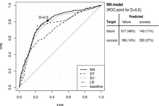
The left of Figure 2 plots the ROC curves for the four models tested. A good model should offer the best compromise between a desirable a high true positive rate (TPR) and low false positive rate (FPR). The former goal cor-responds to a sensitive model, while the latter is related with a more specific model. The advantage of the ROC curve is that the domain user can select the best TPR and FPR trade-off that serves its needs. The NN ROC curve
is related with the highest area (AUC) and outperforms all other methods within most (75%) of the FPR range (e.g., NN is the best method for FPR within [0.00,0.10], [0.26,0.85] and [0.94,1.00]).
Focusing on the case studied of bank telemarketing, it is difficult to finan-cially quantify costs, since long term deposits have different amounts, interest rates and subscription periods. Moreover, human agents are hired to accept inbound phone calls, as well as sell other non deposit products. In addition, it is difficult to estimate intrusiveness of an outbound call (e.g., due to a stressful conversation). Nevertheless, we highlight that current bank context favors more sensitive models: communication costs are contracted in bundle packages, keeping costs low; and more importantly, the 2008 financial crisis strongly increased the pressure for Portuguese banks to increase long term de-posits. Hence, for this particular bank it is better to produce more successful sells even if this involves loosing some effort in contacting non-buyers. Under such context, NN is the advised modeling technique, producing the best TPR and FPR trade-off within most of the sensitive range. For the range FPR within [0.26,0.85], the NN gets a high TPR value (ranging from 0.75 to 0.97). The NN TPR mean difference under the FPR range [0.45,0.62] is 2 pp when compared with SVM and 9 pp when compared with DT. For demonstrative purposes, the right of Figure 2 shows the confusion matrix related with the NN model and for D = 0.5.
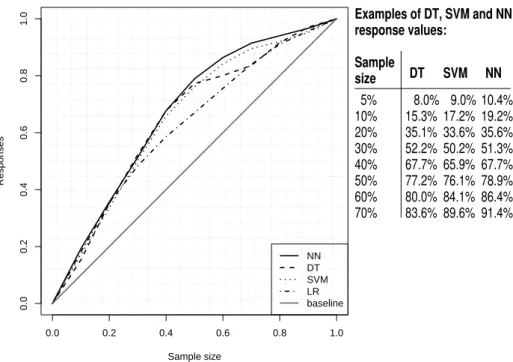
The left of Figure 3 plots the Lift cumulative curves for the predictions using the four models, while the right of Figure 3 shows examples of cumulative lift response values for the best three models (NN, SVM and DT) and sev-eral sample size configurations (e.g., 10% and 50%). Under the cumulative lift analysis, the NN model is the best model within a large portion (77%) of the
0.0 0.2 0.4 0.6 0.8 1.0 0.0 0.2 0.4 0.6 0.8 1.0 FPR TPR ● D=0.5 NN DT SV LR baseline Predicted Target
(ROC point for D=0.5):
NN model success failure failure 617 (48%) 186 (14%) 140 (11%) success 350 (27%)
Fig. 2. ROC curves for the four models (left) and example confusion matrix for NN and D = 0.5 (right)
sample size range. In effect, NN outperforms the SVM model for the sample size ranges of [0.06;0.24] and [0.27;0.99], presenting an average difference of 2 pp within the range [0.27:0.9]. Also, NN is better than DT for the sam-ple size ranges of [0,0.22], [0.33,0.40], [0.46,0.9] and [0.96,1]. The largest NN difference when compared with DT is achieved for the sample size range of [0.46,0.9], reaching up to 8 pp. Since for this particular bank and context the pressure is set towards getting more successful sells (as previously explained), this is an important sample size range. Currently, the bank uses a standard process that does not filter clients, thus involving a calling to all clients in the database. Nevertheless, in the future there can be changes in the bank client selection policy. For instance, one might imagine the scenario where telemar-keting manager is asked to reduce the number of contacts by half (maximum of the bank’s current intentions). As shown in Figure 3, without the data-driven model conceived, telemarketing would reach expectedly just 50% of the possible subscribers, while with the NN model proposed here would allow
to reach around 79% of the responses, thus benefiting from an increase of 29 pp of successful contacts. This result attests the utility of such model, which allows campaign managers to increase efficiency through cost reduction (less calls made) and still reaching a large portion of successful contacts.
0.0 0.2 0.4 0.6 0.8 1.0 0.0 0.2 0.4 0.6 0.8 1.0 Sample size Responses NN DT SVM LR baseline response values: Sample size 10% 5% 70% 20% 30% 40% 50% 60% DT 8.0% 15.3% 35.1% 52.2% 67.7% 77.2% 80.0% 83.6% SVM 10.4% 19.2% 35.6% 51.3% 67.7% 78.9% 86.4% 91.4% NN 9.0% 17.2% 33.6% 50.2% 65.9% 76.1% 84.1% 89.6% Examples of DT, SVM and NN
Fig. 3. Lift cumulative curves for the four models (left) and examples of NN and DT cumulative lift response values (right)
When comparing the best proposed model NN in terms of modeling versus rolling windows phases, there is a decrease in performance, with a reduction in AUC from 0.929 to 0.794 and ALIFT from 0.878 to 0.672. However, such reduction was expected since in the modeling phase the feature selection was tuned based on validation set errors, while the best model was then fixed (i.e., 22 inputs and H = 6) and tested on completely new unseen and more recent data. Moreover, the obtained AUC and ALIFT values are much better than the random baseline of 50%.
3.3 Explanatory knowledge
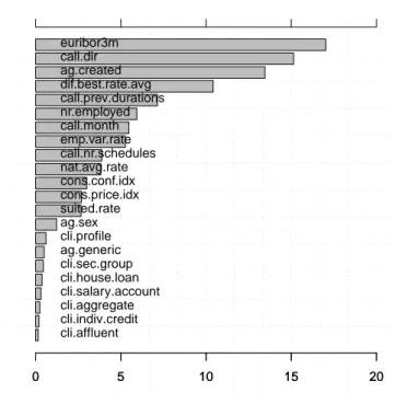
In this section, we show how explanatory knowledge can be extracted by using a sensitivity analysis and rule extraction techniques (Section 2.2) to open the data-driven model. Using the Importance function of the rminer package, we applied the Data-based Sensitivity Analysis (DSA) algorithm, which is capable of measuring the global influence of an input, including its iterations with other attributes [7]. The DSA algorithm was executed on the selected NN model, fitted with all training data (51651 oldest contacts). Figure 4 exhibits the respective input importance bar plot (the attribute names are described in more detail on Table 2). A DT was also applied to the output responses of the NN model that was fitted with all training data. We set the DT complexity parameter to 0.001, which allowed to fit a DT a low error, obtaining a mean absolute error of 0.03 when predicting the NN responses. A large tree was obtained and to simplify the analysis, Figure 5 presents the obtained decision rules up to six decision levels. An example of an extracted rule is: if the number of employed is equal or higher than 5088 thousand and duration of previously scheduled calls is less than 13 minutes and the call is not made in March, April, October or December, and the call is inbound then the probability of success is 0.62. In Figure 5, decision rules that are aligned with the sensitivity analysis are shown in bold and are discussed in the next paragraphs.
An interesting result shown by Figure 4 is that the three month Euribor rate (euribor3m), computed by the European Central Bank (ECB) and published by Thomson Reuters, i.e., a publicly available and widely used index, was considered the most relevant attribute, with a relative importance around 17%. Next comes the direction of the phone call (inbound versus outbound,
cli.affluent cli.indiv.credit cli.aggregate cli.salary.account cli.house.loan cli.sec.group ag.generic cli.profile ag.sex suited.rate cons.price.idx cons.conf.idx nat.avg.rate call.nr.schedules emp.var.rate call.month nr.employed call.prev.durations dif.best.rate.avg ag.created call.dir euribor3m 0 5 10 15 20 0 5 10 15 20
Fig. 4. Relative importance of each input attribute for the NN model (in %)
Fig. 5. Decision tree extracted from the NN model
15%), followed by the number of days since the agent login was created, which is an indicator of agent experience in the bank contact center, although not necessarily on the deposit campaign, since each agent can deal with different types of service (e.g., phone banking). The difference between the best possible rate for the product being offered and the national average rate is the fourth most relevant input attribute. This feature was expected to be one of the top attributes, since it stands for what the client will receive for subscribing the
bank deposit when compared to the competition. Along with the Euribor rate, these two attributes are the ones from the top five which are not specifically related to call context, so they will be analyzed together further ahead. Last in the top five attributes comes the duration of previous calls that needed to be rescheduled to obtain a final answer by the client. It is also interesting to notice that the top ten attributes found by the sensitivity analysis (Figure 4) are also used by the extracted decision tree, as shown in Figure 5.
Concerning the sensitivity analysis input ranking, one may also take into con-sideration the relevance of the sixth and eighth most relevant attributes, both related to social quarterly indicators of employment, the number of employees and the employment variation rate, which reveal that these social indicators play a role in success contact modeling. While client attributes are specific of an individual, they were considered less relevant, with six of them in the bottom of the input bar plot (Figure 4). This does not necessarily mean in that these type of attributes have on general few impact on modeling contact success. In this particular case, the profiling indicators used were defined by the bank and the obtained results suggest that probably these indicators are not adequate for our problem of targeting deposits.
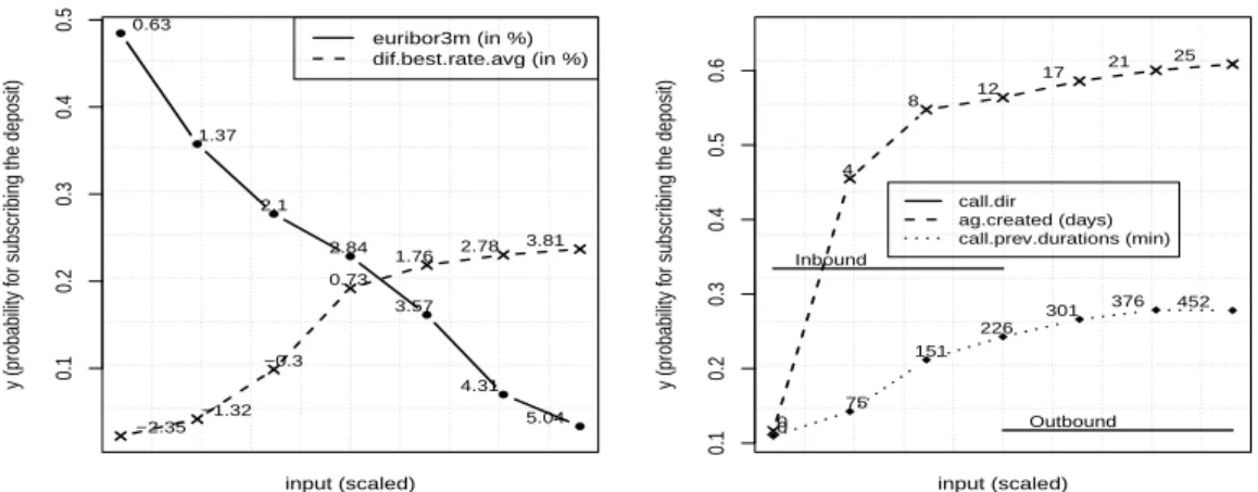
The sensitivity analysis results can also be visualized using a VEC curve, which allows understanding the global influence of an attribute in the pre-dicted outcome by plotting the attribute range of values versus the average sensitivity responses [7]. We analyzed the top five most relevant attributes, with the corresponding VEC curves being plotted in the left (Euribor and product offered interest rates) and right (remaining top 5 relevant attributes) of Figure 6.
0.1 0.2 0.3 0.4 0.5 y (probability f or subscr
ibing the deposit)
● ● ● ● ● ● ● euribor3m (in %) dif.best.rate.avg (in %) input (scaled) 0.63 1.37 2.1 2.84 3.57 4.31 5.04 −2.35 −1.32 −0.3 0.73 1.76 2.78 3.81 0.1 0.2 0.3 0.4 0.5 0.6 y (probability f or subscr
ibing the deposit) call.dir ag.created (days) call.prev.durations (min) input (scaled) Inbound Outbound 0 4 8 12 17 21 25 0 75 151 226 301 376 452
Fig. 6. VEC curves showing the influence of the first and fourth (left) and second, third and fifth (right) most relevant attributes.
When considering the Euribor rate, one might think that a lower Euribor would result in a decline in savings rate since most European banks align their deposits interest rate offers with ECB indexes, particularly with the three month Euribor [27]. Still, the right of Figure 6 reveals the opposite, with a lower Euribor corresponding to a higher probability for deposits subscription, and the same probability decreasing along with the increase of the three month Euribor. A similar effect is visible in a decision node of the extracted DT (Fig-ure 5), where the probability of success decreases by 10 pp when the Euribor rate is higher than 0.73. This behavior is explained by a more recent research [30], which revealed that while prior to 2008 a weak positive relation could be observed between offered rate for deposits and savings rate, after 2008, with the financial crisis, that relation reversed, turning clients more prone to savings while the Euribor constantly decreased. This apparent contradiction might be due to clients perception of a real economic recession and social depression. Consumers might feel an increased need to consider saving for the future as opposed to immediate gratification coming from spending money in purchas-ing desired products or services. This observation emphasizes the inclusion of
this kind of information on similar DM projects. Concerning the difference between best product rate offered and national average, Figure 6 confirms our expectation that an increase in this attribute does increase the probability for subscribing a deposit. Still, once the difference reaches 0.73%, the influence on the probability of subscription is highly reduced, which means that an interest rate slightly above the competition seems to be enough to make the difference on the result. It is also interesting to note that the extracted DT reveals a positive effect of the rate difference with a successful contact (Figure 5).
The right of Figure 6 shows the influence of the second, third and fifth most relevant attributes. Regarding call direction, we validate that clients contacted through inbound are keener to subscribe the deposit. A similar effect is mea-sured by the extracted DT, where an inbound call increases the probability of success by 25 pp (Figure 5). Inbound is associated with less intrusiveness given that the client has called the bank and thus he/she is more receptive for a sell. Another expected outcome is related with agent experience, where the knowledge extraction results show that it has a significant impact on a successful contact. Quite interestingly, a few days of experience are enough to produce a strong impact, given that under the VEC analysis with just six days the average probability of success is above 50% (Figure 6) and the extracted DT increases the probability of successful sell by 9 pp when the experience is higher or equal than 3.3 days (Figure 5). Regarding the duration of previously scheduled calls, it happens often that the client does not decide on the first call on whether to subscribe or not the deposit, asking to be called again, thus rescheduling another call. In those cases (63.8% for the whole dataset), a contact develops through more than one phone call. The sensitivity anal-ysis (Figure 6) shows that more time already spent on past calls within the
same campaign increases probability of success. Similarly, the extracted DT confirms a positive effect of the duration of previous calls. For instance, when the duration is higher or equal than 13 minutes (left node at the second level of Figure 5), then the associated global probability of success is 0.3, while the value decreases to 0.05 (25 pp difference) if this duration condition is false.
It is interesting to note that some explanatory variables are uncontrolled by the commercial bank (e.g., three month Euribor rate) while others are par-tially controlled, i.e., can be influenced by bank managers decisions (e.g., dif-ference between best offered and national average rates, which also depends on competitors decisions), and other variables can be fully controlled (e.g., direction of call, if outbound; agent experience – ag.created; duration of pre-viously scheduled calls). Given these characteristics, telemarketing managers can act directly over some variables, while analyzing expectations influenced by uncontrolled variables. For instance, managers can increase campaign in-vestment (e.g., by assigning more agents) when the expected return is high, while postponing or reducing marketing campaigns when a lower success is globally predicted.
4 Conclusions
Within the banking industry, optimizing targeting for telemarketing is a key issue, under a growing pressure to increase profits and reduce costs. The recent 2008 financial crisis dramatically changed the business of European banks. In particular, Portuguese banks were pressured to increase capital requirements (e.g., by capturing more long term deposits). Under this context, the use of a decision support system (DSS) based on a data-driven model to predict the
result of a telemarketing phone call to sell long term deposits, is a valuable tool to support client selection decisions of bank campaign managers.
In this study, we propose a personal and intelligent DSS that uses a data mining (DM) approach for the selection of bank telemarketing clients. We analyzed a recent and large Portuguese bank dataset, collected from 2008 to 2013, with a total of 52944 records. The goal was to model the success of subscribing a long-term deposit using attributes that were known before the telemarketing call was executed. A particular emphasis was given on feature engineering, as we considered an initial set of 150 input attributes, including the commonly used bank client and product features and also newly pro-posed social and economic indicators. During the modeling phase, and using a semi-automated feature selection procedure, we selected a reduced set of 22 relevant features. Also, four DM models were compared: logistic regression (LR), decision trees (DT), neural networks (NN) and support vector machines (SVM). These models were compared using two metrics area of the receiver operating characteristic curve (AUC) and area of the LIFT cumulative curve (ALIFT), both at the modeling and rolling window evaluation phases. For both metrics and phases, the best results were obtained by the NN, which resulted in an AUC of 0.80 and ALIFT 0.67 during the rolling windows eval-uation. Such AUC corresponds to a very good discrimination. Moreover, the proposed model has impact in the banking domain. For instance, the cumu-lative LIFT analysis reveals that 79% of the successful sells can be achieved when contacting only half of the clients, which translates in an improvement of 29 pp when compared with the current bank practice, which simply contacts all clients. By selecting only the most likely buyers, the proposed DSS cre-ates value for the bank telemarketing managers in term of campaign efficiency
improvement (e.g., reducing client intrusiveness and contact costs).
Two knowledge extraction techniques were also applied to the proposed model: a sensitivity analysis, which ranked the input attributes and showed the av-erage effect of the most relevant features in the NN responses; and a decision tree, which learned the NN responses with a low error and allowed the extrac-tion of decision rules that are easy to interpret. As an interesting outcome, the three month Euribor rate was considered the most relevant attribute by the sensitivity analysis, followed by the direction call (outbound or inbound), the bank agent experience, difference between the best possible rate for the product being offered and the national average rate, and the duration of previ-ous calls that needed to be rescheduled to obtain a final answer by the client. Several of the extracted decision rules were aligned with the sensitivity anal-ysis results and make use of the top ten attributes ranked by the sensitivity analysis. The obtained results are credible for the banking domain and provide valuable knowledge for the telemarketing campaign manager. For instance, we confirm the result of [30], which claims that the financial crisis changed the way the Euribor affects savings rate, turning clients more likely to perform savings while Euribor decreased. Moreover, inbound calls and an increase in other highly relevant attributes (i.e., difference in best possible rate, agent ex-perience or duration of previous calls), enhance the probability for a successful deposit sell.
In future work, we intend to address the prediction of other telemarketing relevant variables, such as the duration of the call (which highly affects the probability of a successful contact [23]) or the amount that is deposited in the bank. Additionally, the dataset may provide history telemarketing behavior for cases when clients have previously been contacted. Such information could
be used to enrich the dataset (e.g., computing recency, frequency and mone-tary features) and possibly provide new valuable knowledge to improve model accuracy. Also it would be interesting to consider the possibility of splitting the sample according to two sub-periods of time within the range 2008-2012, which would allow to analyze impact of hard-hit recession versus slow recovery.
Acknowledgments
We would like to thank the anonymous reviewers for their helpful suggestions.
References
[1] David Arnott and Graham Pervan. Eight key issues for the decision support systems discipline. Decis. Support Syst., 44(3):657–672, 2008.
[2] Leo Breiman, Jerome H Friedman, Richard A Olshen, and Charles J Stone. Classification and regression trees. Wadsworth & Brooks. Monterey, CA, 1984.
[3] David S Coppock. Why lift? data modeling and mining. Inf. Manag. Online, pages 5329–1, 2002. [Online; accessed 19-July-2013].
[4] C. Cortes and V. Vapnik. Support Vector Networks. Mach. Learn., 20(3):273– 297, 1995.
[5] Paulo Cortez. Data mining with neural networks and support vector machines using the r/rminer tool. In Advances in Data Mining. Applications and Theoretical Aspects, volume 6171, pages 572–583. Springer, 2010.
[6] Paulo Cortez, Ant´onio Cerdeira, Fernando Almeida, Telmo Matos, and Jos´e Reis. Modeling wine preferences by data mining from physicochemical
properties. Decis. Support Syst., 47(4):547–553, 2009.
[7] Paulo Cortez and Mark J Embrechts. Using sensitivity analysis and visualization techniques to open black box data mining models. Inform. Sciences, 225:1–17, 2013.
[8] Dursun Delen. A comparative analysis of machine learning techniques for student retention management. Decis. Support Syst., 49(4):498–506, 2010.
[9] Dursun Delen, Ramesh Sharda, and Prajeeb Kumar. Movie forecast guru: A web-based dss for hollywood managers. Decis. Support Syst., 43(4):1151–1170, 2007.
[10] Pedro Domingos. A few useful things to know about machine learning. Commun. ACM, 55(10):78–87, 2012.
[11] Tom Fawcett. An introduction to roc analysis. Pattern Recogn. Lett., 27(8):861– 874, 2006.
[12] Isabelle Guyon and Andr´e Elisseeff. An introduction to variable and feature selection. J. Mach. Learn. Res., 3:1157–1182, 2003.
[13] T. Hastie, R. Tibshirani, and J. Friedman. The Elements of Statistical Learning: Data Mining, Inference, and Prediction. Springer-Verlag, NY, USA, 2nd edition, 2008.
[14] S.S. Haykin. Neural networks and learning machines. Prentice Hall, 2009.
[15] Sadaf Hossein Javaheri, Mohammad Mehdi Sepehri, and Babak Teimourpour. Response modeling in direct marketing: A data mining based approach for target selection. In Yanchang Zhao and Yonghua Cen, editors, Data Mining Applications with R, chapter 6, pages 153–178. Elsevier, 2014.
[16] Philip Kotler and Kevin Lane Keller. Framework for marketing management, 5th Edition. Pearson, 2012.
[17] Kin-Nam Lau, Haily Chow, and Connie Liu. A database approach to cross selling in the banking industry: Practices, strategies and challenges. J. Database Mark. & Cust. Strategy Manag., 11(3):216–234, 2004.
[18] William Leigh, Russell Purvis, and James M Ragusa. Forecasting the nyse composite index with technical analysis, pattern recognizer, neural network, and genetic algorithm: a case study in romantic decision support. Decis. Support Syst., 32(4):361–377, 2002.
[19] David Martens and Foster Provost. Pseudo-social network targeting from consumer transaction data. NYU Working Papers Series, CeDER-11-05, 2011.
[20] David Martens and Foster Provost. Explaining data-driven document classifications. MIS Quarterly, 38(1):73–99, 2014.
[21] David Martens, Jan Vanthienen, Wouter Verbeke, and Bart Baesens. Performance of classification models from a user perspective. Decis. Support Syst., 51(4):782–793, 2011.
[22] M. Moller. A scaled conjugate gradient algorithm for fast supervised learning. Neural Netw., 6(4):525–533, 1993.
[23] S´ergio Moro, Raul Laureano, and Paulo Cortez. Enhancing bank direct marketing through data mining. In Proceedings of the Fourty-First International Conference of the European Marketing Academy, pages 1–8. European Marketing Academy, 2012.
[24] David L Olson, Dursun Delen, and Yanyan Meng. Comparative analysis of data mining methods for bankruptcy prediction. Decis. Support Syst., 52(2):464–473, 2012.
[25] Robert Phillips. Optimizing prices for consumer credit. J. Revenue Pricing Manag., 12:360–377, 2013.
[26] John Platt. Sequential minimal optimization: A fast algorithm for training support vector machines. Technical report msr-tr-98-14, Microsoft Research, 1998.
[27] Gerard O Reilly. Information in financial market indicators: An overview. Q. Bull. Artic. (Central Bank of Ireland), 4:133–141, 2005.
[28] Roland T. Rust, Christine Moorman, and Gaurav Bhalla. Rethinking marketing. Harv. Bus. Rev., 1:1–8, 2010.
[29] R. Setiono. Techniques for Extracting Classification and Regression Rules from Artificial Neural Networks. In D. Fogel and C. Robinson, editors, Computational Intelligence: The Experts Speak, pages 99–114. IEEE Press, 2003.
[30] P Stinglhamber, Ch Van Nieuwenhuyze, and MD Zachary. The impact of low interest rates on household financial behaviour. Econ. Rev. (National Bank of Belgium), 2:77–91, 2011.
[31] Fabrice Talla Nobibon, Roel Leus, and Frits CR Spieksma. Optimization models for targeted offers in direct marketing: Exact and heuristic algorithms. Eur. J. Oper. Res., 210(3):670–683, 2011.
[32] Efraim Turban, Ramesh Sharda, and Dursun Delen. Decision Support and Business Intelligence Systems, 9th Edition. Pearson, 2011.
[33] W. Venables and B. Ripley. Modern Applied Statistics with S. Springer, 4th edition, 2003.
[34] Ian H Witten and Eibe Frank. Data Mining: Practical machine learning tools and techniques, 2nd Edition. Morgan Kaufmann, 2005.
[35] T.F. Wu, C.J. Lin, and R.C. Weng. Probability estimates for multi-class classification by pairwise coupling. J. Mach. Learn. Res., 5:975–1005, 2004.