ADVANCED METHODOLOGIES FOR THE
ASSESSMENT OF THE FATIGUE BEHAVIOUR OF
RAILWAY BRIDGES
Carlos Miguel Correia Albuquerque
2015
Dissertation submitted to the Faculty of Engineering of the University of Porto in fulfilment of the requirements for the degree of Doctor in Civil Engineering.
Supervisor: Rui Artur Bártolo Calçada (Full Professor, FEUP)
À Diana e
ao Francisco,
à Carolina
e aos meus pais
v
ABSTRACT
The relevance of railways as a means of transport of passengers and goods has been increasing over the last decades. This reflects in a number of railway projects that are considered as a priority for the European Union. When assessing the economic viability of such projects, in addition to the high initial cost with the infrastructure construction, there are costs deferred over time that must be accounted for, such as inspection, maintenance, retrofitting and renewal of the track and of the Civil Engineering structures, such as bridges. In this context, fatigue arises as one of the main causes of damage during service life of structures. In the case of steel and composite bridges, it is often reported as the main cause of severe damage.
The research presented in this Thesis aimed at providing new numerical and experimental methodologies that allow the accurate and efficient fatigue assessment of railway bridges. These tools would help Infrastructure Managers to optimise bridge inspection, maintenance and retrofitting interventions, in order to minimise their economic impact.
The work starts by performing a brief historical overview encompassing the main milestones in terms of understanding of the fatigue phenomenon. The typical causes for fatigue damage in bridges are enumerated and some case studies of fatigue damage observed in railway bridges, found in literature, are presented. The fatigue damage assessment methodologies present in the main international standards are debated later, with special emphasis put on the Eurocodes. Alternative and more advanced methodologies for the fatigue analysis are also described. Most
vi
as the parameter governing the stress field at the crack front and, consequently, the crack propagation rate.
The bridge of the new railway crossing of river Sado was used as the case study for the application of the experimental and numerical methods developed. A numerical model of the bridge was built and calibrated based on the results of Ambient Vibration and Load Tests performed in the bridge. A monitoring system was designed and implemented in the structure aiming at characterising traffic and estimating fatigue damage at the critical details identified: the diagonals located in the diaphragms of the deck. Fatigue damage was computed according to linear damage accumulation method present in Eurocode 3. A methodology was developed and incorporated in the monitoring system allowing for the computation of fatigue damage, not only at the directly monitored details (with strain gauges), but also at non-monitored details. The stress state at these non-monitored locations is computed based on the traffic characteristics captured by the monitoring system and on the modal parameters gathered from the calibrated numerical model of the bridge. The results obtained indicate that, for this case study and for the observed traffic volumes, the fatigue damage at the critical locations is very low. Most of the damage is induced by freight trains circulating at low speeds. The contribution of the passenger trains, which typically circulate at speeds above 145 km/h, is almost negligible.
Additionally, a new numerical methodology was developed that allows for the expedite computation of SIF time histories in cracked structures under complex loading. The concept of modal stress intensity factor, required for the application of the proposed methodology, is introduced. The methodology was validated with a simple example, a simply supported beam containing a semi-elliptical crack and subject to dynamic loading. Finally, it was applied to the simulation of a fatigue crack propagation in one of the critical details of the bridge. A local numerical model of the detail, with a finer mesh, was built. Reconciliation with the global model of the bridge was achieved through the implementation of submodelling. A conservative scenario of a pre-existing through-thickness crack, with 15 mm, was considered. The simulation was performed using minimal computational resources. The crack propagation simulation stopped when the maximum simulated SIF achieved the material’s toughness. The results obtained under the above mentioned conservative assumptions and for the current traffic volumes, indicate a remaining fatigue life for the detail of approximately 95 years.
vii
RESUMO
A importância da ferrovia como meio de transporte de pessoas e bens tem aumentado ao longo das últimas décadas. Este facto reflete-se no número de projetos ferroviários considerados prioritários para a União Europeia. Na avaliação da viabilidade económica destes projetos, para além do avultado custo inicial com a construção das infraestruturas, há custos diferidos no tempo a contabilizar, tais como a inspeção, manutenção, reparação e renovação da via e das estruturas de Engenharia Civil, como por exemplo as pontes. Neste contexto, a fadiga surge como uma das principais causas de dano durante a fase de serviço das estruturas, sendo até mesmo reportada como a principal causa de dano severo em pontes de aço e mistas.
A investigação apresentada nesta Tese visa fornecer novas metodologias numéricas e experi-mentais que permitam uma rigorosa e eficiente avaliação da fadiga em pontes ferroviárias. Estas ferramentas poderão ajudar o Gestor das Infraestruturas a otimizar as intervenções de inspeção, manutenção e reparação, de forma a reduzir o seu impacto económico.
Inicialmente apresenta-se uma breve revisão histórica dos principais passos dados em termos da compreensão do fenómeno da fadiga. São enumeradas as causas mais comuns para o dano de fadiga em pontes e são apresentados casos, encontrados na bibliografia, de dano por fadiga em pontes ferroviárias. Posteriormente, são debatidas as metodologias de avaliação do dano por fadiga presentes nos principais códigos internacionais, com especial ênfase nos Eurocódigos. Metodologias alternativas e mais avançadas são também descritas. Maior enfoque é colocado nas
viii
que governa o campo de tensões na frente da fenda e consequentemente a sua taxa de propagação. A ponte da nova travessia ferroviária do rio Sado foi usada como o caso de estudo para aplicação dos métodos numéricos e experimentais desenvolvidos. Um modelo numérico da ponte foi construído e calibrado com base nos resultados de um Ensaio de Vibração Ambiental e de um Ensaio de Carga realizados na ponte. Um sistema de monitorização foi projetado e implementado na estrutura, visando caracterizar o tráfego e estimar o dano de fadiga em detalhes críticos: as diagonais localizadas nos diafragmas do tabuleiro. O dano por fadiga foi calculado com base no método da acumulação linear de dano preconizada pelo Eurocódigo 3. Uma metodologia foi desenvolvida e incorporada no sistema de monitorização permitindo o cálculo do dano por fadiga, não apenas nos detalhes monitorizados diretamente (com extensómetros), mas também nos detalhes não monitorizados. No último caso, o estado de tensão é calculado com base nas características de tráfego capturadas pelo sistema de monitorização e nos parâmetros modais obtidos com o modelo numérico da ponte. Os resultados obtidos indicam que, para o caso de estudo e para o volume de tráfego observado, o dano por fadiga nos detalhes críticos é muito baixo. A maior parte do dano é provocada por comboios de mercadorias que circulam a baixa velocidade. O contributo dos comboios de passageiros, que circulam, tipicamente, a velocidades superiores a 145 km/h, é quase nulo.
Adicionalmente, foi desenvolvida uma nova metodologia numérica que permite calcular, de forma expedita, o histórico do FIT em estruturas com fendas e sujeitas a carregamento complexo. É introduzido o conceito de fator de intensidade de tensão modal, necessário para a aplicação da metodologia proposta. A metodologia foi validada com um exemplo simples, uma viga simplesmente apoiada contendo uma fenda semielíptica e sujeita a um carregamento dinâmico. Posteriormente, foi aplicada à simulação da propagação de uma fenda de fadiga num dos detalhes críticos da ponte. Foi construído um modelo numérico local do detalhe, com uma malha refinada. A compatibilização com o modelo global da ponte foi feita através de técnicas de submodelação. Foi testado um cenário conservador, em que uma fenda inicial, passante, com 15 mm, estava presente no detalhe. A simulação foi realizada utilizando recursos computacionais reduzidos. A simulação da propagação de fenda terminou quando o máximo FIT simulado atingiu a tenacidade do material. Os resultados obtidos com as considerações conservadoras referidas e para o volume de tráfego atual, indicam que o detalhe tenha uma vida à fadiga de aproximadamente 95 anos.
ix
ACKNOWLEDGEMENTS
This Thesis was only possible with the help, support and guidance of several individuals and institutions to whom I owe much gratitude. To all of them I convey my sincere thanks:
To my Supervisor, Professor Rui Calçada, for all the energy and effort put on providing me the conditions to perform this work. I would like to thank all the teachings that highly contributed to my growth in scientific terms, in particular in the areas of numerical and experimental characterization of the dynamic behaviour of structures. I really appreciate all the friendship and support in the different stages of my work and of my life;
To my Co-Supervisor, Professor Paulo Tavares de Castro, for all the teaching, namely on the areas of fatigue and Fracture Mechanics. I would also like to express all the gratitude for the friendship, availability, willingness to help and incentive words throughout the Thesis;
To Professor Raimundo Delgado, for his example, friendship and always kind words. Also for sparking in me the interest for the dynamic behaviour of structures;
To my friend Diogo Ribeiro, for all the fruitful discussions and always valuable comments and inputs. Also for his example of determination and pragmatism;
To Nuno Pinto, for his generosity and for all the support on the set up and installation of the monitoring system of the bridge of the new railway crossing of river Sado;
x
To my friends Joana Delgado, Joel and Pedro Montenegro;
To Diogo Ribeiro, Joel Malveiro, João Francisco Rocha, João Rocha, Nuno Pinto and Nuno Ribeiro for the companionship during the experimental campaigns in the bridge, including the thousands of km driven between Porto and Alcácer do Sal;
To André Paixão, Carlos da Conceição and Carlos Sousa, for the careful review of this Thesis; To my friends and colleagues from our department and research group, for contributing to a very pleasant work environment, where discussion and sharing of experiences benefit each ones work;
To Professor Abílio de Jesus and Luís Silva, for the help, guidance and fruitful collaboration in the last phases of the work. Also for kindly welcoming me at UTAD premises, in Vila Real;
To Professor Álvaro Cunha, for the collaboration in the context of the FADLESS project, for the teaching in the area of experimental methods on structural dynamics and for the several words of esteem and consideration over these years;
To Fernando Marques, for the interesting discussions and collaboration in the context of the FADLESS project;
To Professors Joaquim Gabriel and Teresa Restivo, for the lessons on Instrumentation for Data Measurement, Acquisition and Transmission;
To Professor Miguel Figueiredo, Roberto Miranda and Valentin Richter-Trummer for the fundamental role on the execution of fatigue crack propagation tests;
To the Portuguese Foundation for Science and Technology (FCT), for the funding of the work presented in this Thesis through the scholarship SFRH/BD/47545/2008 and the Research Project “Advanced methodologies for the assessment of the dynamic behaviour of high speed railway bridges” (FCOMP-01-0124-FEDER-007195);
To the European Commission, which funded this same work in the context of the Research Project “FADLESS - Fatigue damage control and assessment for railway bridges” (RFSR-CT-2009-00027);
xi execution of the experimental tests in the bridge;
To Eng. António Reis, designer of the bridge of the new railway crossing of river Sado, for the information provided concerning the design of the structure;
To Teixeira Duarte, S.A., in particular to Eng. Henrique Nicolau, for permitting multiple visits to the bridge during its construction, therefore allowing a better planning of the experimental work performed. Moreover, it was also highly appreciated the availability to provide samples of the steel and welds used on the construction of the critical details of the bridge, which enriched the work performed in this Thesis. In the case of the weld samples, their execution by AMAL is also acknowledged;
To LNEC, in particular to Eng. Luís Oliveira Santos and Eng. João Santos, for the opportunity to perform measurements on the bridge during the load tests performed at the commissioning phase. It is also appreciated the sharing of the results obtained by LNEC during those tests;
To Walter Waes, from Galp Energia, for supporting me in the final stages of this Thesis, seeking its conclusion;
To Professor António Arêde, for the support from the Structural and Seismic Engineering Laboratory, both in terms of personnel and equipment for the experimental campaigns;
To Sr. Valdemar and André for the help on the preparation of the experimental work; To Marta Poinhas and Joana Rodrigues for their always kind and prompt assistance;
Finally, to my family. To my parents, Francisca and José, who always taught me, through words and example, the value of hard work. I’m forever grateful for their effort, understanding and love and for the way they always encouraged me on pursuing this work. To my sister, Carolina, for always being able to make me laugh. Also for her understanding in all the situations where, during this work, I was not as present as I should. To my beloved wife, Diana, for her permanent joy, love, support and patience. Finally, to Francisco, who, without even knowing it, was the final and definitive inspiration to conclude this work.
xiii
CONTENTS
Chapter 1 - Introduction... 1
1.1 CONTEXT... 1
1.2 OBJECTIVES AND SCOPE ... 9
1.3 RESEARCH CONTRIBUTION ... 10
1.4 OUTLINE OF THE THESIS ... 11
Chapter 2 - Fatigue damage of steel and composite bridges ... 13
2.1 INTRODUCTION ... 13
2.2 THE PHENOMENON OF FATIGUE DAMAGE ... 19
2.3 CAUSES FOR FATIGUE DAMAGE OF STEEL AND COMPOSITE BRIDGES ... 28
2.3.1 Presence of defects on the welds ... 28
xiv
2.3.3 Secondary deformations and stresses ... 30
2.3.4 Excessive vibrations ... 31
2.4 EXAMPLES OF FATIGUE DAMAGE ON STEEL AND COMPOSITE BRIDGES ... 31
2.4.1 Eyebars and hangers... 33
2.4.1.1 Silver Bridge ... 34
2.4.1.2 Sungsoo Grand Bridge ... 35
2.4.1.3 Illinois Route 157 Bridge ... 36
2.4.1.4 Bridge over river Skellefte ... 37
2.4.2 Flange gussets and cover-plates ... 38
2.4.2.1 King’s Bridge ... 38
2.4.3 Diaphragms, cross-bracing connections and connections between floor beams and the main load-carrying members ... 39
2.4.3.1 Lafayette Street Bridge ... 39
2.4.3.2 Panaro Bridge ... 41
2.4.3.3 Bridge over river Belle Fourche ... 43
2.4.4 Web penetration and orthotropic decks ... 44
2.4.4.1 Dan Ryan railway viaduct ... 44
2.4.4.2 Maihama Bridge ... 45
2.4.5 Weld defects ... 46
2.4.5.1 Bridge over Quinnipiac River ... 47
2.4.5.2 River Mardle Viaduct ... 48
2.4.5.3 Gulf Outlet Bridge ... 49
2.4.6 Lamellar tearing ... 50
2.4.6.1 Rigid box girder frames of Ft. Duquesne Bridge access viaducts ... 50
xv
2.5 CONCLUDING REMARKS ... 53
Chapter 3 - Standards for the fatigue assessment of railway bridges ... 55
3.1 INTRODUCTION ... 55
3.2 FATIGUE ASSESSMENT ACCORDING TO THE EUROCODES ... 56
3.2.1 Introduction ... 56
3.2.2 Standard fatigue loads and load cases ... 57
3.2.3 Fatigue strength ... 61
3.2.3.1 S-N curves for normal stresses ... 62
3.2.3.2 S-N curves for shear stresses ... 64
3.2.3.3 Partial safety factor for fatigue ... 65
3.2.3.4 Detail categories ... 66
3.2.4 Determination of actuating stresses ... 68
3.2.5 Assessment methods ... 71
3.2.5.1 Equivalent constant amplitude stress range method ... 71
3.2.5.2 Linear damage accumulation method ... 74
3.3 FATIGUE ASSESSMENT ACCORDING TO OTHER INTERNATIONAL STANDARDS... 76
3.3.1 BS5400 - Steel, concrete and composite bridges. Part 10. Code of practice for fatigue… ... 76
3.3.1.1 Introduction ... 76
3.3.1.2 Standard fatigue loads and load cases ... 76
3.3.1.3 Fatigue strength ... 79
3.3.1.4 Determination of actuating stresses ... 83
3.3.1.5 Assessment methods ... 84
3.3.2 AASHTO - LRFD Bridge Design Specifications ... 87
xvi
3.3.2.2 Standard fatigue loads and load cases ... 87
3.3.2.3 Fatigue strength ... 88
3.3.2.4 Assessment methods and other considerations ... 90
3.3.3 International Institute of Welding – Recommendation for Fatigue Design of Welded Joints and Components ... 92
3.3.3.1 Introduction ... 92
3.3.3.2 Fatigue strength ... 93
3.3.3.3 Assessment methods ... 96
3.4 CONCLUDING REMARKS ... 97
Chapter 4 - Advanced methodologies for the fatigue assessment of
structures ... 101
4.1 INTRODUCTION ... 101
4.2 FATIGUE ASSESSMENT BASED ON STRUCTURAL STRAINS AND STRUCTURAL STRESSES 103 4.2.1 Introduction ... 103
4.2.2 General approach ... 103
4.2.3 Dong’s Approach ... 106
4.2.4 Xiao-Yamada Approach ... 108
4.3 FATIGUE ASSESSMENT BASED ON NOTCH STRESSES ... 109
4.3.1 Introduction ... 109
4.3.2 Critical distances approach ... 110
4.3.3 Notch fictitious radius approach ... 111
4.3.4 Highly stressed volume approach ... 112
xvii
4.4.1 Introduction ... 113
4.4.2 General approach ... 114
4.4.2.1 Strength assessment ... 114
4.4.2.2 Loading characterization ... 115
4.4.3 Further improvements to the general approach ... 115
4.5 FATIGUE ASSESSMENT BASED ON FRACTURE MECHANICS AND CRACK PROPAGATION LAWS ... 116
4.5.1 Introduction ... 116
4.5.2 Griffith and the Energy Release Rate, G ... 116
4.5.3 Westergaard and the Stress Intensity Factor, K ... 121
4.5.4 Relationship between the energy release rate and the stress intensity factor ... 126
4.5.5 Fatigue cracks growth as a function of K... 129
4.5.6 Crack propagation retardation laws in LEFM ... 133
4.5.7 Recent advances of the Extended Finite Element Method (XFEM)... 135
4.6 CONCLUDING REMARKS ... 138
Chapter 5 - Crack analysis of dynamically loaded structures using modal
superposition of stress intensity factors ... 141
5.1 INTRODUCTION ... 141
5.2 MODAL SUPERPOSITION OF STRESS INTENSITY FACTORS APPLIED TO THE FATIGUE ANALYSIS ... 143
5.2.1 Dynamic analysis using modal superposition ... 143
xviii
5.2.3 Modal stress intensity factors ... 146
5.2.4 Submodelling ... 148
5.2.5 Computational algorithm ... 149
5.3 APPLICATION ... 152
5.3.1 Introduction ... 152
5.3.2 Description of the structure ... 152
5.3.3 Modal and static stress intensity factors ... 154
5.3.4 Global response ... 157
5.3.4.1 Loading scenario ... 157
5.3.4.2 Time history of K obtained with model BRM ... 158
5.3.4.3 Time history of K obtained with model SSM ... 162
5.4 CONCLUDING REMARKS ... 163
Chapter 6 - Fatigue damage monitoring of the bridge of the new railway
crossing of river Sado ... 165
6.1 INTRODUCTION ... 165
6.2 BRIDGE OF THE NEW RAILWAY CROSSING OF RIVER SADO ... 168
6.2.1 Context ... 168 6.2.2 Description ... 171 6.2.2.1 Structure ... 171 6.2.2.2 Track ... 179 6.2.2.3 Materials ... 180 6.2.3 Construction process ... 180
xix
6.3 NUMERICAL MODEL OF THE BRIDGE ... 188
6.3.1 Description ... 188
6.3.2 Geometrical and mechanical characteristics ... 190
6.3.2.1 Deck ... 190
6.3.2.2 Arches and hangers ... 191
6.3.3 Validation with Ambient Vibration Test ... 193
6.3.3.1 Test Setup ... 193
6.3.3.2 Results ... 194
6.3.4 Validation with Load Tests ... 197
6.3.5 Extraction of relevant modal parameters ... 199
6.4 LONG-TERM MONITORING SYSTEM ... 201
6.4.1 Introduction ... 201
6.4.2 Traffic Characterization Module ... 202
6.4.2.1 Qualitative evaluation ... 202
6.4.2.2 Quantitative evaluation ... 203
6.4.3 Structural Response Characterization Module... 206
6.4.4 Trigger module... 207
6.4.5 Data acquisition and control module ... 207
6.4.6 Communication module ... 208
6.4.7 Database ... 208
6.4.7.1 Determination of Train Speed, Direction and Axles Spacing ... 209
6.4.7.2 Determination of Train Axle Loads... 211
6.4.7.3 Train carriages identification ... 212
xx
6.5 ASSESSMENT OF THE FATIGUE BEHAVIOUR... 213
6.5.1 Methodology ... 213
6.5.2 Traffic characteristics ... 214
6.5.3 Fatigue Damage ... 218
6.5.3.1 Monitored details ... 218
6.5.3.2 Extrapolation for non-monitored details ... 223
6.5.4 Fatigue Damage vs Traffic Characteristics ... 225
6.6 CONCLUDING REMARKS ... 228
Chapter 7 - Advanced fatigue assessment of the bridge of the new railway
crossing of river Sado ... 231
7.1 INTRODUCTION ... 231
7.2 ASSESSMENT OF THE FATIGUE CRACK PROPAGATION STRENGTH ... 233
7.2.1 Fatigue crack growth tests... 233
7.2.1.1 Experimental details ... 233
7.2.1.2 Discussion of the results ... 238
7.2.2 Fractographic analysis... 243
7.2.2.1 Experimental details ... 243
7.2.2.2 Discussion of the results ... 249
7.3 SIMULATION OF FATIGUE CRACK PROPAGATION ... 252
7.3.1 Theoretical background ... 252
7.3.2 Proposed workflow for residual fatigue life assessment of bridge details ... 254
xxi
7.3.3.1 Identification of the critical detail ... 258
7.3.3.2 Local monitoring of the critical detail ... 259
7.3.3.3 The global numerical model of the bridge ... 260
7.3.3.4 The numerical model of the critical detail and shell-to-solid sub-modelling ... 261
7.3.3.5 Fatigue model assumptions ... 263
7.3.4 Analysis and discussion of results ... 263
7.3.4.1 Experimental Validation ... 263
7.3.4.2 Comparison of stress intensity factor’s computation techniques ... 266
7.3.4.3 Computation of residual fatigue life ... 266
7.4 CONCLUDING REMARKS ... 270
Chapter 8 - Conclusions ... 273
8.1 GENERAL CONCLUSIONS ... 273
8.2 FUTURE DEVELOPMENTS ... 281
xxiii
LIST OF FIGURES
Figure 1.1 – Passenger journey times vs. distance: rail vs air transport (EC, 2010). ... 2 Figure 1.2 – Tran-European Transport Network: core network corridors (EC, 2013). ... 3 Figure 1.3 – Planned railways in Portugal (EC, 2013): (a) freight and (b) passenger lines. ... 4 Figure 2.1 - Forced landing of a Boeing 737 due to partial ejection of the aircraft’s fuselage as a consequence of the unstable propagation of fatigue cracks (NTSB, 1989). ... 15 Figure 2.2 - Brittle fracture of a vessel due to unstable propagation of fatigue cracks (Hayes, 1996). ... 15 Figure 2.3 – Steel pipeline after long crack propagation (Makino et al., 2001). ... 16 Figure 2.4 - Derailment of ICE train due to fatigue damage at a wheel of one of the train’s axles (O'Connor, 2007): (a) derailment and (b) location of fatigue cracks. ... 17 Figure 2.5 - Fatigue cracks on rails (Magel et al., 2004): (a) rail-wheel contact and (b) fatigue crack. ... 17 Figure 2.6 – Collapse of the Silver Bridge (Bennett and Mindlin, 1973): (a) bridge before collapse, (b) bridge after collapse, (c) point of failure and (d) fractured eye-plate. ... 18 Figure 2.7 - Effect of crack propagation retardation under variable loading conditions (Schijve, 2003): (a) crack propagation retardation and (b) effective stresses around the crack. ... 22 Figure 2.8 - Experimental results of variable amplitude fatigue tests (Schijve, 2003). ... 23 Figure 2.9 - Phases of fatigue damage (Radaj et al., 2006). ... 24 Figure 2.10 – Schematic representation of the orders of magnitude of the fatigue problem (Broek, 1987). ... 24
xxiv
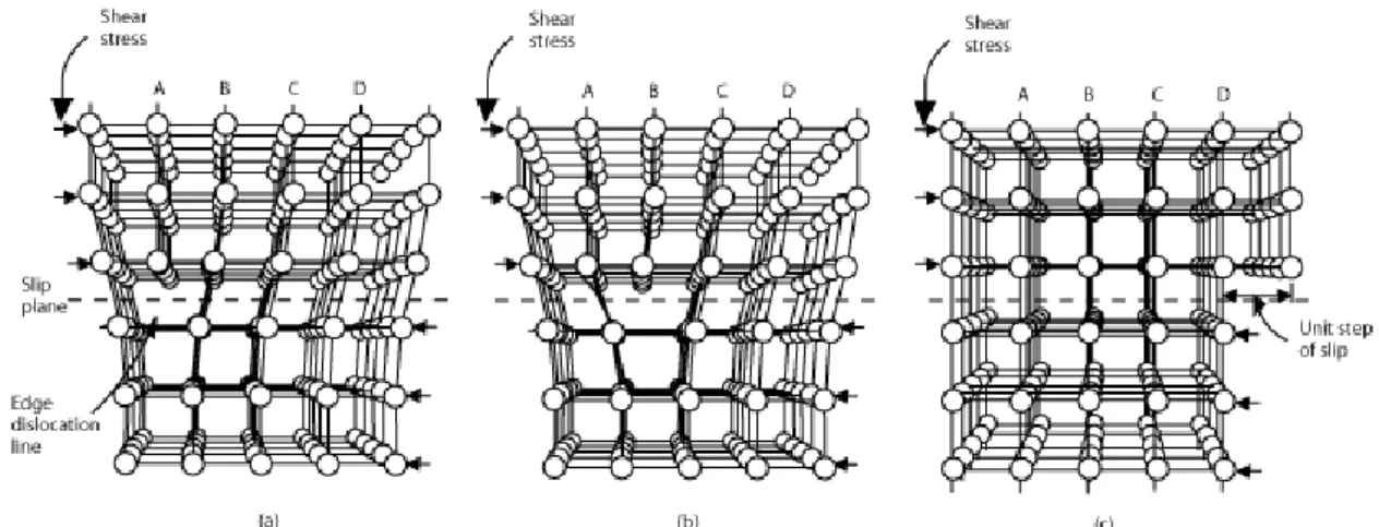
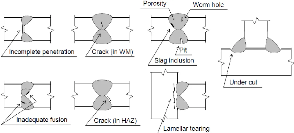
Figure 2.11 - Illustration of the atomic dislocations phenomenon (NDTRC, 2014). ... 25 Figure 2.12 - Cracks initiation and micro-cracks propagation: (a) generation of extrusions and intrusions (NDTRC, 2014) and (b) micro-crack and crack propagation from extrusions and intrusions (ESDEP, 1996). ... 25 Figure 2.13 - Fatigue striation: (a) example of a fracture surface with fatigue striation (ESDEP, 1996) and (b) process of striation generation (NDTRC, 2014). ... 26 Figure 2.14 - Fatigue cracks surface: (a) relation between cyclic loading and crack surface striation appearance (de Castro and Meggiolaro, 2009a) and (b) striation on the fracture surface of a structural steel (Richter-Trummer et al., 2011). ... 27 Figure 2.15 - Ductile fracture: (a) cavitation phenomenon (de Castro and Meggiolaro, 2009a) and (b) ductile fracture surface (Richter-Trummer et al., 2011). ... 28 Figure 2.16 - Different types of defects found in welds (Miki, 2010). ... 29 Figure 2.17 - Crack initiation in the welds due to stress concentrations (ESDEP, 1996): (a) stress concentrations on the weld and (b) potential crack locations. ... 29 Figure 2.18 - Example of main and secondary connection forces (Miki, 2010). ... 31 Figure 2.19 - Categorization of fatigue failures of steel bridges (Haghani et al., 2012). ... 32 Figure 2.20 - Schematic elevation view of the Silver Bridge (Fisher, 1984). ... 34 Figure 2.21 - Eye-plate of the Silver Bridge after collapse (Fisher, 1984): (a) eye-plate and (b) fracture surface. ... 35 Figure 2.22 – Elevation view of the collapsed Sungsoo Grand Bridge (Cho et al., 2001). ... 35 Figure 2.23 – Typical connection of vertical hanger (Cho et al., 2001). ... 36 Figure 2.24 - Illinois Route 157 Bridge (Fisher, 1984): (a) perspective of one suspended segment and (b) scheme of a hanger. ... 37 Figure 2.25 - Bridge over the river Skellefte and hanger-to-arch connection (Al-Emrani and Kliger, 2009). ... 38 Figure 2.26 - King’s Bridge, Melbourne, Australia (Miki, 2010): (a) overview and (b) typical cross-section. ... 38 Figure 2.27 - Cover-plate at King’s Bridge (Miki, 2010): (a) cover-plate and (b) schematic of the crack propagation. ... 39 Figure 2.28 - Bridge of Lafayette street (Fisher, 1984). ... 40 Figure 2.29 - Fatigue crack at the Lafayette Bridge (Fisher, 1984): (a) fatigue crack and (b) schematics of the crack propagation. ... 40
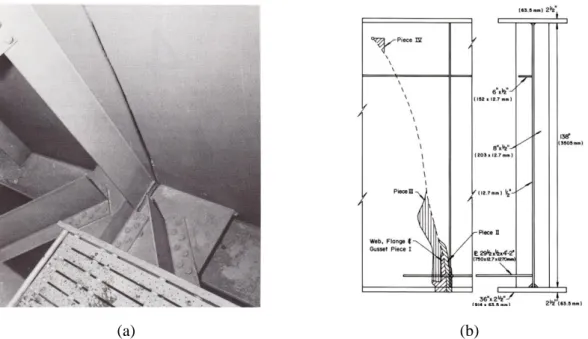
xxv Figure 2.30 - Fatigue crack initiation zone (Fisher, 1984): (a) fractured section and (b) stages of the crack propagation. ... 41 Figure 2.31 – Panaro Bridge (Lippi et al., 2011). ... 41 Figure 2.32 – Distortion induced fatigue crack at track’s cross beam (Lippi et al., 2011). ... 42 Figure 2.33 – Vibration induced fatigue crack at sleepers-longitudinal girder connection (Lippi et al., 2011). ... 42 Figure 2.34 - Fatigue crack initiation zone (Fisher, 1984): (a) fractured section and (b) stages of the crack propagation. ... 43 Figure 2.35 - Fatigue cracks in the bridge crossing the river Belle Fourche (Fisher, 1984): (a) fractured detail and (b) schematics of crack propagation. ... 43 Figure 2.36 - Dan Ryan railway viaduct (Fisher, 1984): (a) overview and (b) structure of the deck. ... 44 Figure 2.37 - Fatigue cracks at the Dan Ryan railway viaduct (Fisher, 1984): (a) crack’s typical location and (b) detail of the crack. ... 45 Figure 2.38 - Cross section of the Maihama bridge (Miki, 2010) ... 45 Figure 2.39 - Typical locations of fatigue cracks observed in the Maihama bridge (Miki, 2010)
... 46 Figure 2.40 - Bridge over river Quinnipiac (Fisher, 1984) ... 47 Figure 2.41 - Fatigue crack at the bridge over river Quinnipiac (Fisher, 1984): (a) visible crack and (b) fatigue crack propagation stages. ... 48 Figure 2.42 – Elevation view of River Mardle Viaduct (Clubley and Winter, 2003). ... 48 Figure 2.43 – Cross section of one of the box girders (Clubley and Winter, 2003). ... 49 Figure 2.44 - Gulf Outlet bridge (Fisher, 1984): (a) overview and (b) cross section. ... 49 Figure 2.45 - Location of fatigue cracks of Gulf Outlet bridge (Fisher, 1984): (a) cross section of one of the deck’s box girder, (b) core extracted and (c) visible location of the crack. ... 50 Figure 2.46 - Rigid box girder frames of the Ft. Duquesne Bridge’s access viaducts (Lindberg and Schultz, 1997): (a) overview and (b) design. ... 51 Figure 2.47 - Fatigue crack due to lamellar tearing (Fisher, 1984): (a) schematics of crack development and (b) observed crack... 51 Figure 2.48 - Fatigue cracks initiated in holes filled with filler material. ... 52
xxvi
Figure 2.49 - Fatigue cracks in components with change in section: (a) due to tension and (b) due to shear stresses. ... 52 Figure 3.1 - Example of a fatigue train: Train Type 1 – Locomotive-hauled passenger train (CEN, 2003)... 57 Figure 3.2 - Load model LM71 (CEN, 2003). ... 59 Figure 3.3 - Flow chart for determining whether a dynamic analysis is required (CEN, 2003). 60 Figure 3.4 - S-N curves for direct stress ranges (CEN, 2004). ... 63 Figure 3.5 - Alternative strength curve for details with special classification, ΔσC* (CEN, 2004).
... 64 Figure 3.6 - S-N curves for shear stress ranges (CEN, 2004). ... 65 Figure 3.7 - Details described in “Table 8.4: Weld attachments and stiffeners” of (CEN, 2004).
... 67 Figure 3.8 - Details described in “Table B.1: Detail categories for use with geometric (hot spot) stress method” of (CEN, 2004). ... 68 Figure 3.9 - Nominal stress example (ESDEP, 1996)... 69 Figure 3.10 - Modified nominal stress example. ... 69 Figure 3.11 – Geometric (hot spot) stress (Radaj et al., 2006). ... 69 Figure 3.12 - Relevant stresses at fillet welds (CEN, 2004). ... 70 Figure 3.13 - Workflow of the linear damage accumulation method (CEN, 2004). ... 75 Figure 3.14 – Example of train (Train 9) considered in RU type of loading (BSI, 1980). ... 77 Figure 3.15 - Example of train (Train 1) considered in RL type of loading (BSI, 1980). ... 77 Figure 3.16 - Typical R – N relationship (BSI, 1980). ... 79
Figure 3.17 - Summary of mean-line R – N curves (adapted from BSI (1980)). ... 81
Figure 3.18 - R – N curves of detail class E for different probabilities of failure (adapted from
BSI (1980)). ... 82 Figure 3.19 - Example of classification of non-welded details (BSI, 1980). ... 83 Figure 3.20 - Reference stress in parent metal (BSI, 1980). ... 84 Figure 3.21 – Example of stress concentration factors provided in Appendix H of BS5400 (BSI, 1980)... 84 Figure 3.22 – S-N curves specified in AASHTO standard (AASHTO, 2012). ... 89 Figure 3.23 - Example of detail categories for Load-Induced Fatigue (adapted from AASHTO (2012)). ... 90
xxvii Figure 3.24 – S-N curves for normal stresses and standard applications (IIW, 2008). ... 94 Figure 3.25 – S-N curves for normal stresses and very high cycles applications (IIW, 2008). .. 94 Figure 3.26 – S-N curves for shear stresses (IIW, 2008). ... 95 Figure 3.27 – Example of fatigue resistance classification against nominal stresses (IIW, 2008).
... 95 Figure 3.28 – Example of fatigue resistance classification against hot spot stresses (IIW, 2008).
... 96 Figure 4.1 - Range of applicability of different methodologies of fatigue analysis (Radaj et al., 2006). ... 102 Figure 4.2 - Structural stress (Radaj et al., 2006). ... 104 Figure 4.3 - Structural stress measurement in hollow section connections (Radaj et al., 2006): (a) conditioning geometric parameters and (b) proposed distances. ... 104 Figure 4.4 - Structural stress/strain measurements in welded connections of plain elements (Radaj et al., 2006): (a) conditioning geometric parameters and (b) reference distances. ... 105 Figure 4.5 - Example of finite element models of welded connections between plain components and points for the stress/strain assessment (Radaj et al., 2006): (a) model using shell elements and (b) model using volume elements. ... 105 Figure 4.6 - Geometric and loading variables influencing the definition of stress concentration factors (Radaj et al., 2006): (a) hollow section connections and (b) cope hole at I-section girder. ... 106 Figure 4.7 - Structural stress strength curves for tubular joints (Radaj et al., 2006). ... 106 Figure 4.8 - Through thickness linearization of stresses, according to Dong: (a) elements with normal thickness (Dong, 2001), (b) element with high thickness or welded connection to the lateral surface of a plate (Dong, 2005) and (c) symmetric welded connection (Dong, 2001). ... 107 Figure 4.9 - Linearization of stresses according to Dong (Radaj et al., 2006): (a) linearization through the entire thickness and (b) linearization through a fraction of the thickness. 107 Figure 4.10 - Fatigue strength curve according to Dong (Radaj et al., 2009). ... 108 Figure 4.11 - Xiao-Yamada approach (Xiao and Yamada, 2004): (a) reference detail, with t = 10 mm, (b) plate with dimensions different from reference and (c) corresponding S-N curve. ... 108
xxviii
Figure 4.12 - Stress concentration factor (Kt) vs. Fatigue notch factor (Kf) (Radaj et al., 2006). ... 109 Figure 4.13 - Notch fictitious radius method: (a) computation of structural stresses (Radaj et al., 2006), (b) plane model with fictitious notch rounding (Fricke, 2012) and (c) transference of the internal forces to the plane model (Radaj et al., 2006). ... 112 Figure 4.14 - Basic hypothesis of the notch strain approach (Radaj et al., 2006). ... 113 Figure 4.15 - Strain S-N curves (Dowling, 2007): (a) generic curve and (b) strain S-N curve for a structural steel. ... 114 Figure 4.16 - Strain energy per unit volume, for uniaxial stress. ... 117 Figure 4.17 - Strain energy per unit volume at a plate under uniaxial stress (Parker, 1981): (a) uncracked plate under uniaxial stress and (b) cracked plate. ... 118 Figure 4.18 – Change in energy as a function of cracks length (Parker, 1981). ... 119 Figure 4.19 – Theoretical resistance of a material under traction (Branco et al., 1999): (a) schematics of a cubic lattice, (b) relative coordinates of 2 consecutive atoms, (c) displacement vs. atomic force and (d) atomic σ-ε curve. ... 120 Figure 4.20 – Infinite plate with a crack perpendicular to the direction of loading. ... 122 Figure 4.21 – Change of the coordinates system to the crack tip. ... 125 Figure 4.22 – Modes I, II and III of crack propagation. ... 126 Figure 4.23 – Closure of the crack tip (Broek, 1987). ... 127 Figure 4.24 – Generic relationship between crack propagation rate and stress intensity factor range (adapted from Roylance (2001)). ... 131 Figure 4.25 – Information required for a fatigue crack propagation analysis (Albuquerque et al., 2012a). ... 132 Figure 4.26 – Parameters intervening in the Wheeler model (Broek, 1987). ... 135 Figure 4.27 – Enriched nodal sets for cracks (adapted from Fries and Belytschko (2010)). .... 137 Figure 5.1 - Criteria for the definition of the Ksta and Kj signs. ... 148
Figure 5.2 - Flow chart for the application of the proposed methodology: (a) with submodelling and (b) without submodelling. ... 151 Figure 5.3 - Geometric properties of the application: (a) beam dimension and crack location [m] and (b) crack dimensions (section A-A) [m]. ... 152 Figure 5.4 - Finite element model BRM: (a) overview and (b) zoom to the mesh near the crack.
xxix Figure 5.5 - Finite element models SSM: (a) overview of the global coarse shell model and (b) local refined brick model. ... 153 Figure 5.6 - Crack front: major points A and B and location based on angle Φ (adapted from Murakami (1987)). ... 154 Figure 5.7 - Modal stress intensity factors through the crack front and corresponding mode shapes. ... 156 Figure 5.8 - Static stress intensity factor through the crack front. ... 157 Figure 5.9 - Contribute of the static loading and of the different modes of vibration to Ktotal(t) at
point B. ... 159 Figure 5.10 - Total response: Ktotal(t) and Ktotal*(t): (a) at point A and (b) at point B. ... 160
Figure 5.11 - Results comparison between novel and conventional methodologies: (a) at point A and (b) at point B... 161 Figure 5.12 - Results comparison between the novel methodology and the application of the expressions of Newman and Raju: (a) at point A and (b) at point B. ... 161 Figure 5.13 - Results comparison between the BRM and SSM models: (a) at point A and (b) at point B. ... 162 Figure 6.1 - Bridge of the new railway crossing of the river Sado: (a) location (REFER, 2011) and (b) overview (REFER, 2010). ... 169 Figure 6.2 - Alcácer Bypass: different routes studied and final commissioned route (solution F) (REFER, 2010) ... 170 Figure 6.3 - Annual cargo movement in the sea port of Sines (Porto de Sines, 2015) ... 171 Figure 6.4 - Side elevation of the 2nd span of the bridge (GRID et al., 2006). ... 171
Figure 6.5 - Cross section of the deck (GRID et al., 2006). ... 172 Figure 6.6 - Diaphragms of the deck: typical details. ... 173 Figure 6.7 - Spherical hinge at hanger to deck connection. ... 174 Figure 6.8 - Concrete slab (GRID et al., 2006) ... 174 Figure 6.9 - Arches: cross section variation (GRID et al., 2006). ... 175 Figure 6.10 - Arches: (a) inside view and (b) diaphragms and stiffeners (GRID et al., 2006). 175 Figure 6.11 - Inspection access to the interior of the arches (GRID et al., 2006). ... 176 Figure 6.12 - Vertical stiffeners bellow the arches’ extremities (GRID et al., 2006). ... 176 Figure 6.13 - Cross section of the piers (GRID et al., 2006): (a) floor-plan and (b) floor-plan including foundations. ... 177
xxx
Figure 6.14 - Pier P2: (a) side elevation (GRID et al., 2006), (b) actual photograph (REFER, 2010) and (c) front elevation (GRID et al., 2006). ... 178 Figure 6.15 - Platforms for piers inspection: (a) design (GRID et al., 2006) and (b) actual .... 178 Figure 6.16 - Pre-stressed concrete sleepers (SATEPOR, 2011). ... 179 Figure 6.17 - Ballasted track located at the upstream side of the bridge. ... 180 Figure 6.18 - Span of the bridge being assembled, over the South access viaduct (REFER, 2010).
... 181 Figure 6.19 - Assembly of the 3 main parts of each elementary unit of the deck (Teixeira Duarte - Engenharia e Construções S.A., 2009). ... 181 Figure 6.20 - Assembly of the parts of the dowels of the deck: (a) webs and bottom flange (Teixeira Duarte - Engenharia e Construções S.A., 2009) and (b) diaphragms and top flanges. ... 182 Figure 6.21 - Welding processes adopted at the construction site (Teixeira Duarte - Engenharia e Construções S.A., 2009): (a) submerged arc welding and (b) MIG/MAG process with Rail Track. ... 182 Figure 6.22 - Dowel’s levelling: (a) dowel over the pulling platform and (b) levelling apparatus.
... 183 Figure 6.23 - Dowels positioning: (a) complimentary dowels, (b) gap control and (c) apparatus for gap control (Teixeira Duarte - Engenharia e Construções S.A., 2009). ... 183 Figure 6.24 - Welding workshop at the pulling platform: (a) steel box exiting workshop and (b) last dowel... 184 Figure 6.25 - Deck’s launching: (a) launching platform and (b) launching nose. ... 184 Figure 6.26 - Temporary piers. ... 185 Figure 6.27 - Elevation of the segments of one arch (REFER, 2010). ... 185 Figure 6.28 - Springing of one arch (REFER, 2010). ... 185 Figure 6.29 - Bottom hinge before nailing (REFER, 2010). ... 185 Figure 6.30 - Removal of the temporary piers (REFER, 2010). ... 186 Figure 6.31 - Concreting of a ballast-guard. ... 186 Figure 6.32 - Track’s construction: (a) sleepers, (b) expansion joint and (c) downstream vs. upstream tracks. ... 186 Figure 6.33 - Catenary and signalling system (REFER, 2010). ... 187
xxxi Figure 6.34 - Details classification according to fatigue: (a) upper (top) extremity and (b) lower (bottom) extremity of the diagonal. ... 187 Figure 6.35 – Numerical model of the bridge of the new railway crossing of river Sado (1st span).
... 188 Figure 6.36 - Numerical model of the bridge: (a) deck and arch’s ending point and (b) cut view of the deck and arch. ... 189 Figure 6.37 - Modelling of diaphragms and diagonals: (a) refined and (b) not refined. ... 189 Figure 6.38 – Cross section of the numerical model of the concrete slab. ... 190 Figure 6.39 – Modelling of the arch and hangers: (a) side elevation of the 2nd span and (b) front elevation of the bridge. ... 191 Figure 6.40 - Monitored points. ... 194 Figure 6.41 - Measurement directions: (a) arch’s section and (b) deck’s section. ... 194 Figure 6.42 - Model update: (a) difference between fnum and fexp and (b) objective function as a
function of Young Modulus of concrete. ... 195 Figure 6.43 - 1st vertical bending mode of vibration. ... 195
Figure 6.44 - 2nd vertical bending mode of vibration... 195
Figure 6.45 - 3rd vertical bending mode of vibration. ... 196 Figure 6.46 - 4th vertical bending mode of vibration. ... 196 Figure 6.47 – Power engine machine (1500 series): (a) distances between axles, average load per axle and (b) overview in the context of the load test performed. ... 197 Figure 6.48 - Double hopper ballast container: (a) distances between axles, average load per axle and (b) overview in the context of the load test performed. ... 197 Figure 6.49 - Single hopper ballast container: (a) distances between axles, average load per axle and (b) overview in the context of the load test performed. ... 198 Figure 6.50 - Long freight train loading positions (adapted from LNEC (2011)). ... 198 Figure 6.51 - Experimental vs. Numerical strain (at position of SG 51-1) due to long freight train static loading. ... 199 Figure 6.52 - Experimental vs. Numerical strain (at position of SG 51-1) due to power engine machine quasi-static loading. ... 199 Figure 6.53 - Location of the different components of the system. ... 201 Figure 6.54 - IP camera installed in a hanger. ... 202
xxxii
Figure 6.55 - IP camera recorded images: (a) Alfa Pendular passengers train, (b) intercity passengers train and (c) freight train. ... 202 Figure 6.56 - Fibre optic rail pad sensors (FORPS): (a) overview and (b) in place. ... 203 Figure 6.57 - Location and labelling of the instrumented rail pads and strain gauges in the rails.
... 203 Figure 6.58 - Instrumented rail pad sensors structure (1 – interference grid (grating), 2 – fibre optic, 3 – elastomer) (SensorLine, 2008) ... 204 Figure 6.59 - Instrumented rail pad sensor signal. ... 204 Figure 6.60 - Strain gauges in the rails: (a) location, (b) welding and (c) protection. ... 205 Figure 6.61 - Signal of full Wheatstone bridges at S2 and S3: (a) τS2 and τS3 and (b) Δτ = τS3 - τS2.
... 206 Figure 6.62 - Location of strain gauges: (a) instrumented sections and (b) nomenclature of strain gauges at Diaphragm 51. ... 207 Figure 6.63 - Data acquisition and control module. ... 208 Figure 6.64 - Filtered transmittance relative variation. ... 210 Figure 6.65 - Detection of peaks of differential shear strain. ... 212 Figure 6.66 - Workflow for fatigue damage computation. ... 214 Figure 6.67 - Histogram of trains’ speed. ... 215 Figure 6.68 - Histogram of trains’ length. ... 216 Figure 6.69 - Histogram of axle loads... 217 Figure 6.70 - Histogram of the load of the trains per unit length. ... 217 Figure 6.71 - Histogram of the number of axles per train... 218 Figure 6.72 - Experimental and numerical stresses for 3 different traffic events stored at the database. ... 219 Figure 6.73 - Dispersion of Alfa Pendular axle load measurements. ... 220 Figure 6.74 - Dispersion of Alfa Pendular numerical simulation results: (a) SG 51-1 and (b) SG 54-1... 220 Figure 6.75 - Example of numerical simulation of response at SG 54-1, with increasing number of modes of vibration. ... 221 Figure 6.76 - Cumulative damage at diagonals 51 and 54: (a) detail at the top of the diagonal and (b) detail at the bottom of the diagonal. ... 222
xxxiii Figure 6.77 - Histograms of stress ranges for numerical and field records at the diagonals of Diaphragms 51 and Diaphragm 54. ... 222 Figure 6.78 - Diaphragms with the most critical non-monitored diagonals. ... 223 Figure 6.79 - Simulated stress history at non-instrumented details of the bridge: (a) traffic event 1 and (b) traffic event 2. ... 223 Figure 6.80 - Cumulative damage for non-instrumented details of the bridge – Category 45. 224 Figure 6.81 - Cumulative fatigue damage after 565 traffic events – Category 45. ... 225 Figure 6.82 - Damage (Diaph. 51 and 54, Cat. 45) vs. Train load per unit length. ... 226 Figure 6.83 - Damage (Diaph. 51 and 54, Cat. 45) vs. Speed of the train. ... 226 Figure 6.84 - Damage (Diaph. 51 and 54, Cat. 45) vs. Total load of the train. ... 227 Figure 6.85 - Damage (Diaph. 51 and 54, Cat. 45) vs. Length of the train. ... 227 Figure 6.86 - Damage (Diaph. 51 and 54, Cat. 45) vs. Number of axles of the train. ... 228 Figure 7.1 - CT specimen... 234 Figure 7.2 - Schematic representation of the location of specimens containing weldments. ... 234 Figure 7.3 - Vickers hardness measurements: (a) hardness and (b) macrostructure. ... 236 Figure 7.4 - Base material da/dN vs. K data for the three R values tested. ... 237 Figure 7.5 - Example of a vs. N data obtained – case of a BM specimen tested under R = 0.1, showing crack lengths on both sides (a1 and a2) and average crack value a. ... 237
Figure 7.6 - Fracture surface in the end of the test (HAZ, R = 0.1). ... 238 Figure 7.7 - Representation of the two exemplary cases studied for determination of the influence of the not-cracked zone on different crack lengths. ... 239 Figure 7.8 - Residual stress perpendicular to the surface where the crack is expected to grow (Richter-Trummer and de Castro, 2011); the max. and min. residual stress values (MPa) are indicated in the vertical axis. ... 241 Figure 7.9 - Weld material da/dN vs. K data for the three R values tested (‘cor’ - Keff). ... 242
Figure 7.10 - Heat affected zone material da/dN vs. K data for the three R values tested (‘cor’ -
Keff). ... 242
Figure 7.11 - Partial representation of the specimen half where micrographs have been taken for analysis of the initial crack growth region. ... 244 Figure 7.12 - Assembly of the micrographs taken in the initial crack growth zone (HAZ, R = 0.1, CT2). ... 245
xxxiv
Figure 7.13 - Example representation of measurements performed for striation spacing determination (HAZ, R = 0.1, CT2). ... 246 Figure 7.14 - Micrograph of the end zone of propagation, showing a typical ductile rupture (HAZ, R = 0.1, CT2). ... 246 Figure 7.15 - Micrograph of a zone of propagation where neither striations nor ductile rupture were found (HAZ, R = 0.1, CT2). ... 247 Figure 7.16 - Striation spacing (s) versus crack length (a) for specimen CT2. ... 247 Figure 7.17 - Striation spacing (s) versus crack length (a) for specimen CT3. ... 248 Figure 7.18 - Relation between results obtained by macroscopic and microscopic measurements for specimen CT3. ... 249 Figure 7.19 - Distance between striations s vs. da/dN for both tested specimens compared to literature data (CT2 - HAZ, R = 0.1 and CT3 - base material, R = 0.4). ... 251 Figure 7.20 - Crack loading modes intervening in mixed mode (I+II) crack propagation: (a) Mode I (opening mode) and (b) Mode II (sliding mode). ... 253 Figure 7.21 - Workflow 1st step: pre-processing of the input data. ... 256
Figure 7.22 - Workflow 2nd step: crack propagation simulation. ... 257
Figure 7.23 - Critical detail to fatigue damage: (a) cross-section of the deck and (b) critical detail. ... 259 Figure 7.24 - Schematic representation of the local weld features of the critical detail: (a) actual weld connection and (b) Eurocode 3 detail category. ... 259 Figure 7.25 - Location of strain gauges at diaphragm 51: (a) global and local strain gauges - schematics and (b) local strain gauges – location and labelling (dimensions in mm). . 260 Figure 7.26 - Local finite element model. ... 262 Figure 7.27 - Shell-to-solid sub-modelling: fit of the local model (in grey) on the global model.
... 262 Figure 7.28 - Strains at the location of the local SG: Experimental vs Numerical. ... 264 Figure 7.29 - Fatigue crack initiation spot: (a) numerical simulation vs. (b) tested experimental joints (Silva et al., 2013). ... 265 Figure 7.30 - Computation of K(t): VCCT vs. DE methods: (a) KI(t) and (b) KII(t). ... 266
Figure 7.31 - Fatigue crack propagation path. ... 267 Figure 7.32 - Crack propagation length as a function of cumulative traffic. ... 268 Figure 7.33 - Crack propagation length vs Time. ... 269
xxxv
LIST OF TABLES
Table 2.1 – Main cause of damage in Civil Engineering structures (adapted from Kühn et al. (2008)). ... 14 Table 2.2 – ATLSS survey of cracking in bridges (Walker et al., 1992). ... 33 Table 2.3 – Minnesota (USA) Department of Transportation survey of cracking in bridges (Lindberg and Schultz, 1997). ... 33 Table 2.4 – Collection of fatigue damage cases in bridges. ... 53 Table 3.1 – Standard fatigue trains (adapted from CEN (2003)). ... 57 Table 3.2 – Standard traffic mix (adapted from CEN (2003)). ... 58 Table 3.3 – Heavy traffic mix (adapted from CEN (2003)). ... 58 Table 3.4 – Light traffic mix (adapted from CEN (2003)). ... 58 Table 3.5 – Partial safety factor for fatigue strength, γMf (CEN, 2004). ... 66 Table 3.6 – Example of k1 factors, for circular hollow sections, in order to account for secondary moments (CEN, 2004). ... 70 Table 3.7 – λ1 for different traffic scenarios (CEN, 2006). ... 73 Table 3.8 – 𝜆2 for different traffic volumes (CEN, 2006). ... 73 Table 3.9 – 𝜆3 for different design lives (CEN, 2006). ... 73 Table 3.10 – λ4 for n = 12% and for different values of ∆σ1∆σ1+2 (CEN, 2006). ... 74 Table 3.11 – RU loading: heavy traffic mix (adapted from BSI (1980)). ... 77
xxxvi
Table 3.12 – RU loading: medium traffic mix (adapted from BSI (1980)). ... 78 Table 3.13 – RU loading: light traffic mix (adapted from BSI (1980)). ... 78 Table 3.14 – RL loading: traffic mix (adapted from BSI (1980)). ... 78 Table 3.15 – σr-N relationships constants (adapted from BSI (1980)). ... 81
Table 3.16 – Probability factors (adapted from BSI (1980)). ... 81 Table 3.17 – Load combinations and load factors (AASHTO, 2012). ... 88 Table 3.18 – Detail Category Constant, A (adapted from AASHTO (2012)). ... 89 Table 3.19 – Constant Amplitude Fatigue Thresholds (adapted from AASHTO (2012)). ... 89 Table 3.20 – Temperature Zone Designations for Charpy V-notch Requirements (AASHTO, 2012). ... 92 Table 3.21 – Fracture Toughness Requirements (AASHTO, 2012). ... 92 Table 5.1 – Natural frequencies of vertical bending vibration modes: BRM vs. SSM. ... 154 Table 6.1 – Additional mass associated to the track and non-structural elements of the deck’s slab. ... 190 Table 6.2 – Geometric characteristics of the diagonals present at the diaphragms. ... 191 Table 6.3 – Geometric characteristics of the hangers. ... 191 Table 6.4 – Geometric characteristics of the 1st arch. ... 192 Table 6.5 – Geometric characteristics of the 2nd arch. ... 192 Table 6.6 – Geometric characteristics of the 3rd arch. ... 193 Table 6.7 – Natural frequencies and modal damping coefficients. ... 196 Table 7.1 – Chemical composition of the S355NL steel (base material). ... 235 Table 7.2 – Some mechanical proprieties of the base material. ... 235 Table 7.3 – C, m and R2 for the several specimens. ... 243 Table 7.4 – Adopted parameters for fatigue analysis. ... 263
1
Chapter 1
INTRODUCTION
1.1 CONTEXT
The relevance of railways as a mean of transport of passengers and goods has been increasing over the last decades. This is due to some advantages of railways when compared to alternative means of transport, such as roadway and airway. Those advantages are economic, environmental and safety related: lower costs of transport; lower energy consumption and CO2 emissions; very
low number of incidents and accidents reported. Also, as the speed of railway traffic increases, it becomes competitive for a wider range of distances. In the case of passenger traffic, in particular, this is boosted by the increased comfort provided by railways and by the development of high-speed railways, with speeds higher than 250 km/h (Figure 1.1). In the case of freight traffic, the development of dedicated freight routes also contributes for the reduction of the time of transportation.
2
Figure 1.1 – Passenger journey times vs. distance: rail vs air transport (EC, 2010).
The above mentioned advantages have been reflecting in: i) increasing volume of passengers and goods transported per year; ii) increasing share of railway traffic when compared to other types of transport systems; iii) increasing loads per train and per train’s axle; iv) expansion of railway networks in many different countries.
In the context of the European Union, the benefits of railways in terms of cost reduction and economic and social cohesion across national boundaries are also acknowledged. The railway sector is expected to take on a larger share of transport demand in the next decades. That intention is reflected in the number of railway projects that are considered as a priority, in the Trans-European Transport Network project (EC, 2013).
Portugal is also to be included in the Trans-European Transport Network. It will connect to the rest of Europe through the Atlantic corridor (in yellow in Figure 1.2).
3 Figure 1.2 – Tran-European Transport Network: core network corridors (EC, 2013).
In the last decades, the country invested in the modernization of some of the rail lines available. The line connecting the two most populous cities, Lisbon and Oporto, was recently upgraded, allowing the increase of speed of conventional trains to around 220 km/h.
Additionally, Portugal has been preparing to install, in the next 2 decades, a few high-speed railway lines, which will allow connecting the country to the European high-speed railway network. Lines specially dedicated to freight traffic are also foreseen. The planned freight and high-speed passenger routes are illustrated in Figure 1.3.
4
(a) (b)
Figure 1.3 – Planned railways in Portugal (EC, 2013): (a) freight and (b) passenger lines.
In addition to the high initial cost with the infrastructure construction, there is a cost that is deferred over time which refers to the inspection, maintenance, retrofitting and renewal of the track and of the Civil Engineering structures, such as bridges. In current days, more than half of the expenditure with infrastructure, in Europe, is related with maintenance and modernization of the existing infrastructure (Kühn et al., 2008). Therefore, and as the ageing process of structures continues, the economic and social relevance of an efficient and effective assessment of infrastructures structures is increasing.
In this context, fatigue arises as one of the main causes of damage during the service life of structures (Oehme, 1989). In the case of steel and composite bridges, it is often reported as the main cause of severe damage (Miki, 2010, Fisher, 1984, Al-Emrani and Kliger, 2009, Cremona et al., 2013, Clubley and Winter, 2003, Cho et al., 2001, Leander et al., 2010, Hai, 2006, Kühn et al., 2008, Wang et al., 2012). The growing speed of trains leads to dynamic amplification effects that accelerate structural degradation, by increasing the number of stress cycles and their amplitudes. Also, as traffic loads also tend to increase, the problem is even more relevant, becoming one of the main topics of investigation of several research projects, such as Details
5 (Chellini et al., 2009), Sustainable Bridges (Cremona et al., 2007), FADLESS (Lippi et al., 2011) and Mainline (Paulsson, 2013).
The fatigue assessment methodologies present in most of the standards are based on S-N curves and linear damage accumulation rules, derived from Palmgren-Miner rule (Miner, 1945). That is the case of the Eurocodes (CEN, 2004). But those approaches, in spite of their easy employment at the design phase, lack effective applicability when dealing with in-service structures. When fatigue damage, e.g. fatigue cracks, are found in those structures, the S-N curves do not allow computing the corresponding remaining fatigue life of the damaged component and structure. Also, they do not help defining the time lapses between inspections or the time available before maintenance and retrofitting measures are required.
On the other hand, the Infrastructure Managers and Railway Operators require that inspection, maintenance and retrofitting interventions are optimised, in order to minimise their economic impact. Line closures are expected to be as short as possible. Therefore, new experimental and numerical fatigue assessment methodologies are required in order to: i) support Infrastructure Manager decision making and planning for interventions; ii) increase safety in railway operations; iii) reduce the costs associated with infrastructure maintenance.
Current investigations focus on both the experimental characterization and numerical assessment of fatigue.
As mentioned before, most standards and procedures, e.g. (CEN, 2004, AASHTO, 2012), quantify fatigue strength on the basis of S-N curves and of linear damage accumulation concepts. This approach, based on the global stress level, is used to predict fatigue life until total failure and is widely spread as a result of its straightforward application; it presents, however, some important limitations. On the one hand, the applicable rules cover a limited number of structural details. On the other hand, the development of S-N curves for new details implies performing tests at the real scale, and these are expensive and time consuming, and consequently generally unpractical for the timings of design and construction (Fricke and Paetzold, 2010, Lotsberg and Landet, 2005, Ling and Pan, 1997). Furthermore, S-N curves are a result of tests that present an important scatter (Pedersen et al., 2010). As a safeguard against this effect the S-N curves are usually very conservative (Casavola and Pappalettere, 2009, Morel and Flacelière, 2005). Finally, fitness for purpose assessments cannot be carried out on the basis of that approach. For a given situation of damage, such as a fatigue crack identified during some non-destructive
6
inspection, the approach does not provide a risk assessment of that defect nor the useful remaining life (Byers et al., 1997). It does not contribute, therefore, for an improved definition of intervals between inspections (Ayala-Uraga and Moan, 2007). Other limitations of the S-N approaches were identified by several authors, concerning, for example, variable amplitude loading (Johannesson et al., 2005), or fatigue life for a very high number of load cycles (Sonsino, 2007).
Alternative approaches developed for the analysis of fatigue are based on local behaviour (Radaj et al., 2009). That is the case of the approaches based on structural stresses, structural strains, notch stresses, notch strains and Fracture Mechanics.
The application of these methodologies to the assessment of large structures poses significant challenges, which limited its use in the context of Civil Engineering structures. Usual calculations involve the application, to the structural detail of interest, of a known loading history under load or displacement control. Computation of the corresponding local stress or strain fields allows for the calculation of fatigue damage indicators. However, for some structures, the loading history is most of the times complex and the corresponding structural dynamical response is unknown in most – or even all – points of interest.
In these circumstances, even when the loading history is known, its effects in the detail under study can only be determined through dynamic analysis of the complete structure. Those analyses are generally based upon the finite element method. The algorithms for solving the numerical problem, as Newmark (Bathe, 1996) or HHT (Chung and Hulbert, 1993), require, frequently, the calculation of thousands of load steps, leading to very time consuming calculation process. High computational costs are heightened as a result of the need for highly refined finite elements meshes in the neighbourhood of the damage locations. That level of refinement cannot be extended to the remaining structure (Chan et al., 2003). This is a problem inherent to the scale difference between the detail where fatigue damage occurred or is likely to occur, of the order of mm or less, and the global structure, that may be of the order of km (Li et al., 2007).
This scale problem is also reflected in the experimental assessments. Since fatigue damage is localised at critical details of the structures, the most usual way for the infrastructure managers to assess it is by periodical or extraordinary bridge inspections (Righiniotis, 2006). When fatigue damage is detected, e.g. fatigue cracks, or expected, the actual condition of the bridge is often assessed by load tests and short term monitoring (Leander et al., 2010, Wang et al., 2012, Lippi
7 et al., 2011, Nagy et al., 2013, Zhou et al., 2013, Caglayan et al., 2009, Brencich and Gambarotta, 2009, Marques et al., 2009, Stamatopoulos, 2013, Srinivas et al., 2013, Fu and Zhang, 2011, Tecchio et al., 2013). In some cases the short term monitoring is also performed during the subsequent repair, strengthening and/or replacement activities (Rodrigues et al., 2012) or even later, to assess the improvements resulting from the retrofitting/enhancement measures (Andersson et al., 2013). The data obtained during the short term monitoring of fatigue prone structures is analysed and, commonly, used to extrapolate the results for longer periods of time (Zhou, 2006).
Nevertheless, it is not economically feasible to perform interventions in all underperforming bridges, at the same time. Their advanced assessment (structural health monitoring - SHM), by means of long-term monitoring systems could help on the prioritization and on the scheduling of inspections and interventions (Orcesi and Frangopol, 2011, Wong, 2012). Advances in technology, such as the development of industrial computers, the wireless communication systems (Picozzi et al., 2010) and the enhancement of all types of electronic transducers, helped increasing the number of applications of long-term monitoring systems to critical structures worldwide (Magalhães et al., 2008, Cross et al., 2013). The benefits of structural health monitoring are quantifiable (Orcesi and Frangopol, 2013) and, in some countries, the use of long-term monitoring systems is even being addressed by regulations (Moreu et al., 2012).
Most of the long-term monitoring systems are focused on detecting damage events (Cury and Crémona, 2012). As the objectives of the SHM become more ambitious, towards damage localization (Whelan and Janoyan, 2010, Dilena and Morassi, 2011, Glisic and Inaudi, 2012), damage severity assessment (Santos et al., 2013) and lifetime prediction update, the complexity of the systems and of the data analysis algorithms also increases.
The long-term monitoring of the global dynamic properties of the structures is one of the most common methods to try to detect the structural damage (Santos, 2014, Rahmatalla et al., 2014, Caglayan et al., 2011, Magalhães et al., 2012b, Ko et al., 2002). In this context, some attempts were made in the past to replace the installation of sensors in the bridge by the utilization of instrumented test vehicles (Van Bogaert, 2012).
An alternative approach is to use a long-term monitoring system that measures strain at a number of details considered of relevance in order to estimate cumulative damage (Costa and Figueiras, 2012, Guo and Chen, 2013, Ye et al., 2012, Xu et al., 2012, Chen et al., 2012, Ni et
8
al., 2012, Guo and Chen, 2011, Liu et al., 2010, Hakola et al., 2012) or even to detect it (Phares et al., 2013, Yao and Glisic, 2012).
Some structures, as the Tsing Ma Bridge, due to their relevance and scale, have long-term monitoring systems that combine the monitoring of their global dynamic behaviour with the local monitoring of strains (Chan et al., 2006, Li et al., 2012).
A structural health monitoring system should be able to perform damage quantification but also to relate the damage with the external actions that originated it. This is the reason why the traffic characterization is a feature of paramount importance in a permanent monitoring system (Guo et al., 2012) to be implemented either in a roadway or in a railway bridge. It allows to understand the type of traffic that has the biggest impact on the structural degradation and to forecast traffic evolution (Fu and You, 2011). The measurement of real traffic also allows avoiding the use of conservative standard load models, when assessing damage evolution and planning inspections frequency (Ottosson et al., 2012a). In the case of railway bridges, the analysis of the transversal positioning of the vehicles is highly simplified, when compared to roadway bridges, since trains are constrained to the rail track.
Several methods for railway traffic characterization are available. The Weight-In-Motion (WIM) techniques try to assess the vehicles geometry by interpreting measurements performed directly in the railway track (Meli and Pugi, 2013). Some common WIM technologies are: i) rail shear measurements using shear strain gauges welded or bonded to the neutral axis of the rail (Julián Valerio, 2005); ii) rail shear measurements, achieved by means of a circular slot drilled on the neutral line of the rail (Esveld, 2001); iii) rail bending measurements (Sekuła and Kołakowski, 2012); iv) instrumented rail pads (SensorLine, 2008). An alternative approach, the Bridge Weight-In-Motion (B-WIM), uses the structural response of the bridge to compute the vehicles geometry and axles load, after a proper calibration process (Karoumi et al., 2005, Liljencrantz et al., 2007, Seo et al., 2013).
As a complement to the SHM systems, in order to forecast the structural behaviour/degradation, due to fatigue or other causes, the development of well-calibrated numerical models of the structure is considered a very important step (Vincenzi et al., 2012, Chen et al., 2011). The calibration of a numerical model may be performed with experimental data resulting from the long-term monitoring system (Gomez and Feng, 2012, He et al., 2008) or from a short term one (Ribeiro et al., 2012, Schlune et al., 2009).
9 As underlined by Guo et al. (2012), the numerical model also plays an important role by allowing to extend the SHM results to the fatigue assessment of non-monitored details. Methodologies based on the influence line concept and that allow achieving those objectives are presented in (Orcesi and Frangopol, 2010) and (Zeng et al., 2012). Other alternative approach explored in the past, was to assume constant relations between the maximum stresses in different details of the bridge, and use those relations as scale factors to convert the damage measured at instrumented details into damage in the remaining points of the structure (Hakola et al., 2012). Finally, in other cases, the simulation of numerical models with real traffic was performed (He et al., 2008).
The above mentioned methodologies lack, in some cases, accuracy, and in other cases are not computationally efficient. That is the reason why, in the past, tracking fatigue damage in all critical details of long-span railway bridges was not achievable in an efficient and economical way.
The current thesis aims to provide new numerical and experimental methodologies that overcome the limitations presented above. The objectives and scope are detailed on the next Section.
1.2 OBJECTIVES AND SCOPE
As mentioned in Section 1.1, the global objective of the current thesis is to provide new numerical and experimental methodologies that allow the accurate and efficient fatigue assessment of railway bridges.
The global objective was achieved through a set of intermediate goals:
Review the methodologies for the fatigue assessment of railway bridges available in the relevant standards;
Review the advanced fatigue assessment methodologies available in literature;
Develop a new numerical approach for the fatigue assessment of railway bridges, based on advanced methodologies found in literature;
Develop a numerical model of the case study and calibrate it based on experimental measurements;