Analysis of a Typical Offshore Tubular KT-Joint to Evaluate the SCF and SIF Values.

(1)

ANALYSIS OF A TYPICAL OFFSHORE TUBULAR

KT-JOINT TO EVALUATE THE SCF AND SIF

VALUES

João Nuno da Silva Pedro Castanheira da Costa

Dissertation submitted to

Faculdade de Engenharia da Universidadedo Porto For the degree of:

Mestre em Engenharia Mecânica

Supervisor: Prof. José A.F.O. Correia (University of Porto, Portugal)

Supervisors: Prof. Abilio M.P. De Jesus (University of Porto, Portugal)

Prof. Dimitrios G. Pavlou (University of Stavanger, Norway)

Mestrado integrado em Engenharia Mecânica

Especialização em Projeto e Construção Mecânica

(2)

(3)

iii

(4)

iv

Acknowledgments

The realization of this thesis could never have been conceivable without the help, support and motivation of a few people to whom I leave my much-appreciated gratitude.

First of all, I would like to express my sincere thankfulness to my thesis supervisor Doctor José António Correia for all the assistance and valuable lessons and advices given during the time of the realization of this thesis.

Secondly, to Professor Dimitios G. Pavlou I leave a special thanks for the extraordinary welcoming and all the help and accessibility showed in the explanation and sharing of information. Furthermore, I would like to express my acknowledgements to all my co-supervisors, Prof. Abílio De Jesus and Prof. Dimitrios Pavlou, who also gave crucial contributes to this master thesis.

The last but not the least, a debt of gratitude to the engineers Paulo Jorge Carmona Mendes and António Mourão for all the time and help made available as well as wise councils for the most entangled issues that may have had risen in the realization of this thesis.

I would like to express my acknowledgements to FCT - Fundação para a Ciência e Tecnologia which supported this work through national funds; UID/ECI/047 08/2019 – CONSTRUCT – Instituto de I&D em Estruturas e Construções funded by national funds through the FCT/MCTES (PIDDAC); and ERASMUS+ program.

I additionally thank the Faculty of Engineering of the University of Porto (FEUP) and the University of Stavanger (Norway) for their support and facilities that were made available to me.

At long last, a major thanks to my friends, family and girlfriend, for the incredible quality and bolster they have constantly given me along my scholarly course.

João Costa September 04, 2019

(5)

v

Agradecimentos

A realização desta tese nunca poderia ter sido concebível sem a ajuda, apoio e motivação de algumas pessoas a quem quero expressar a minha sincera gratidão. Em primeiro lugar, eu gostaria de exprimir a minha gratidão sincera ao meu supervisor de tese doutor José António Correia por toda a toda a ajuda, valiosas lições e conselhos dados durante a realização desta tese.

Em segundo lugar, ao professor Dimitios G. Pavlou deixo um especial obrigado pelas extraordinárias boas-vindas e toda a ajuda e a acessibilidade mostradas na explicação e compartilha de informação. Além disso, gostaria de expressar meus agradecimentos a todos os meus co-orientadores, Prof. Abílio De Jesus e Prof. Dimitrios Pavlou, que também deram contribuições cruciais para esta tese de mestrado.

Por último mas não menos importante, a minha total gratidão aos Engenheiros Paulo Jorge Carmona Mendes e António Mourão por todo o tempo e ajuda postos à disposição bem como sábios concelhos para as questões mais complexas que poderiam surgir na realização da tese.

Eu gostaria de expressar os meus agradecimentos à FCT - Fundação para a Ciência e Tecnologia que suportou este trabalho através de fundos nacionais; UID/ECI/047 08/2019 – CONSTRUCT – Instituto de I&D em Estruturas e Construções financiado por fundos nacionais através do FCT/MCTES (PIDDAC); e ao programa ERASMUS+.

Agradeço ainda à Faculdade da Engenharia da Universidade do Porto (FEUP) e à Universidade de Stavanger (Noruega) pela ajuda e por facultar as instalações para a realização deste trabalho.

Finalmente, os meus sinceros agradecimentos aos meus amigos, família e namorada, pela grande força e pelo apoio incondicional que constantemente me deram ao longo do meu percurso académico.

João Costa 04 de Setembro de 2019

(6)

(7)

vii

Abstract

The organization of increasingly sustainable power source all around the globe is bringing about huge vitality security, environmental change relief and loads of monetary advantages. Support structures are thought to be one of the main drivers for reducing costs in order to make the wind industry more economically efficient. Foundations and towers should be fit for purpose, extending their effective service life but avoiding costs of oversizing. Most of the offshore platforms are normally fixed to seabed and constructed as a truss framework with tubular members as structural elements. The area around the tubular joint has been highly considered among engineers. The stress concentration and stress intensity are the primordial factors in the study of fatigue design. This work was developed with the purpose of studying both stress concentration factors (SCF) and stress intensity factors (SIF) for the typical offshore KT-joint based either on the parametric equations proposed by Lloyd and Efthymiou for the SCF, and IIW, BS7910 and SINTAP standards for SIF. To do a proper study on the matter, an exhaustive and extensive review and state was made. In this way, comparisons between the analytical and numerical solutions were done.

KEYWORDS: Offshore Engineering, Tubular Joint, Hot-Spot Stress, Stress Concentration Factor, Stress Intensity Factor, Parametric Equations

(8)

(9)

ix

Resumo

A organização de uma fonte de energia cada vez mais sustentável em todo o mundo está a trazer uma enorme vitalidade de segurança, atenuação da mudança ambiental e balanços monetários favoráveis. As estruturas de apoio são pensadas para ser um dos principais impulsionadores para a redução de custos a fim de tornar a indústria eólica mais economicamente eficiente. As fundações e as estruturas devem ser adequadas ao propósito estendendo a sua vida de serviço duma forma eficaz evitando custos de sobredimensionamento. A maioria das plataformas offshore são fixadas ao fundo do mar e construídos como estrutura do tipo treliça com membros tubulares servindo de elementos da estrutura. A área em torno da junta tubular tem sido altamente considerada e investigada por engenheiros. O fator de concentração de tensões e o fator de intensidade de tensões são os fatores primordiais no estudo de vida à fadiga. Este trabalho foi desenvolvido com o objetivo de estudar tanto o fator de concentração de tensões (SCF) como o fator de intensidade de tensões (SIF) de uma ligação tubular KT, quer com base nas equações paramétricas propostas por Loyd e Efthymiou para o primeiro parâmetro, e nas normas IIW, BS7910 e SINTAP para o SIF. Para fazer um estudo adequado sobre o assunto, uma revisão exaustiva e extensa foi feita. Assim, comparações foram feitas entre as soluções analíticas e numéricas para os parâmetros em estudo.

PALAVRAS-CHAVE: Engenharia Offshore, Ligação Tubular, Tensões Hot-Spot, Fator de Concentração de Tensões, Fator de Intensidade de Tensões, Equações paramétricas

(10)

(11)

xi

General Index

1. Introduction ... 1 1.1 Motivation ... 1 1.2 Objectives ... 1 1.3 Outline of thesis... 2

2. Review on tubular offshore structures and fatigue assessment methods ... 3

2.1 Introduction ... 3

2.2 Offshore tubular joints ... 4

2.2.1 Introduction ... 4

2.3 Fatigue of offshore structures ... 6

2.3.1 Introduction ... 6

2.3.2 Damage accumulation method ... 9

2.3.3 Nominal stress approach ... 9

2.3.4 Hot-Spot stress approach ... 11

2.3.4.1 Type “a” hot-spots ... 12

2.3.4.2 Type “b” hot-spots ... 13

2.4 Definition of stress concentration factor (SCF) ... 14

2.5 Definition of stress intensity factor (SIF) ... 15

2.6 Estimation of SCF and SIF values based on design codes ... 17

2.6.1 Superposition of stresses in tubular joints ... 17

2.6.2 Parametric equations ... 19

2.6.2.1 Efthymiou equations ... 19

2.6.2.2 Lloyd’s Register equations ... 23

2.6.3 Calculation of SIF by IIW standards ... 23

2.6.4 Calculation of SIF by BS 7910 standards ... 24

2.7 Review on finite element analysis to evaluate the SCF and SIF values of tubular joints ... 26

3. Evaluation of SCF values of a typical tubular KT-joint based on numerical simulation ... 30

3.1. Introduction ... 30

3.2. Geometry of the Tubular KT-joint under consideration ... 30

3.3. SCF evaluation based on DNVGL code/Efthymiou parametric equations ... 32

3.4. SCF evaluation based on Lloyd’s register (LR) equations ... 35

3.5. SCF evaluation based on numerical analysis ... 40

3.6. Conclusions ... 58

4. Evaluation of SIF values of a typical tubular KT-joint ... 61

4.1. Introduction ... 61

(12)

xii 4.2.1 BS7910 standard rules ... 61 4.2.2 Results ... 64 4.2.2.1 Brace B1 ... 64 4.2.2.2 Brace B2 ... 69 4.2.2.3 Brace B3 ... 71

4.3. SIF evaluation based on IIW recommendations ... 75

4.3.1 Rules from IIW recommendations ... 75

4.3.2 Results ... 78

4.3.3.1 Brace B1 ... 78

4.3.3.2 Brace B2 ... 79

4.3.3.3 Brace B3 ... 81

4.4 SIF evaluation on SINTAP standard ... 82

4.4.1 SINTAP standard Rules ... 82

4.4.2 Results ... 85

4.4.2.1 Brace B1 ... 85

4.4.2.2 Brace B2 ... 89

4.4.2.3 Brace B3 ... 90

4.5. Comparison and discussion ... 95

5. Conclusions and future works ... 99

5.1 Conclusions ... 99

5.2 Future works ... 99

(13)

xiii

List of figures

Figure 1 - Piled Structure and Gravity Structure of Brent [4]. ... 3

Figure 2 - Types of offshore structures [4]. ... 4

Figure 3 - Types of tubular joints along with their nomenclature [8]... 5

Figure 4 – Offshore tubular joints: (a) Example of offshore jacket structure; (b) Definition of the geometrical parameters of a joint; (c) Different types of IPB loadings [9]. ... 6

Figure 5 - S-N curves for offshore connections or details based on DNVGL standard [10]. ... 7

Figure 6 - Definition of nominal stress distribution in chord and brace side [1]. ... 7

Figure 7 - Definition of geometric stress distribution in chord and brace side [1]. ... 8

Figure 8 - Definition of notch stress distribution in chord and brace side [1]. ... 9

Figure 9 - Nominal stress approach for assessing the fatigue strength and service life of non-welded structural components [12]. ... 10

Figure 10 - Definition of hot-spot stress [15]. ... 11

Figure 11 - Stress distribution through the thickness of the weld toe and its components [17]. ... 11

Figure 12 - Reference points at different types of meshing [17]... 14

Figure 13 - Stress concentration in tubular joint [8]... 15

Figure 14 - Illustration of arbitrary KT-Joint with definition of saddle and crown points [1]. ... 17

Figure 15 - Superposition of stresses [24]. ... 18

Figure 16 - Stress intensity factor for surface cracks [17]. ... 24

Figure 17 - Examples of welded joints [28]. ... 25

Figure 18 - Stress intensity magnification factor 𝑀𝑏 for surface flaws in bending [28]. ... 25

Figure 19 – Complete profile solid FE T-joint model [15]. ... 27

Figure 20 – Case study a) Jacket-type offshore structure and b) KT-type tubular joint [26]. ... 31

Figure 21 - Solid model with designation of the braces [26]. ... 42

Figure 22 - Solid model with the principal stress points [26]. ... 42

Figure 23 - Solid model with the details of the size of the 8-nodes cube solid elements and 6-nodes triangular solid elements in braces and chord, respectively in the blue zone, 0.15m (Exterior zone) [26]. ... 43

Figure 24 - Solid FE model with the details of the size of the 8-nodes solid elements in green with 5E-2 meters in size [26]. ... 43

Figure 25 - Solid FE model with the designed meshing refinement (Front view) [26]. ... 43

Figure 26 - Solid FE model with the designed meshing refinement (Side view) [26]. ... 43

Figure 27 - Solid FE model with the designed meshing refinement (Top view) [26]. ... 43

Figure 28 - 3D FE model of the KT-Joint under consideration [26]. ... 44

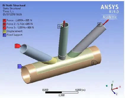
Figure 29 - Solid model with the representation of the axial forces [26]. ... 46

Figure 30 - Details about the support conditions used in the FE model: a) Fixed support; b) Displacement. [26]. ... 46

Figure 31 - Solid model with identification of fixed support [26]. ... 47

Figure 32 - Solid model with identification of restricted and free directions [26]. ... 47

Figure 33 - Stress fields for axial loading case in the KT-joint under consideration [26]. ... 48

Figure 34 - Stress fields for axial loading case in the KT-joint under consideration (Closer look) [26]. . 48

Figure 35 - Stress distribution in brace B1 for axial loading case: Side 1 [26]. ... 49

(14)

xiv

Figure 47 - Stress distribution in chord for axial loading case [26]. ... 55

Figure 48 - Path stresses in chord crown for axial loading case [26] ... 56

Figure 49 - Path stress in brace crown B1 for axial loading case (Side 1 and 2) [26] ... 57

Figure 50 - Path stress in brace saddle B1 for axial loading case (Side 3 and 4) [26] ... 57

Figure 51 - Path stress in brace crown B2 for axial loading case (Side 1 and 2) [26]. ... 57

Figure 53 - Path stress in brace crown B3 for axial loading case (Side 1 and 2) [26] ... 58

Figure 55 - Surface flaw [27]. ... 62

Figure 56 - SIF vs. a curves for the Brace B1 using BS7910 standard based on Lloyd’s Register, DNV standard, and FEA: 𝑎/𝑐 = 0.1. ... 65

Figure 61 - SIF vs. a curves for the Brace B1 using BS7910 standard based on DNV standard for 𝜎𝑛 = 12.5𝑀𝑃𝑎: 0.1 ≤ 𝑎/𝑐 ≤ 0.5. ... 68

Figure 63 - SIF vs. a curves for the Brace B1 using BS7910 standard based on DNV standard for 𝜎𝑛 = 12.5𝑀𝑃𝑎: 1.2 ≤ 𝑎/𝑐 ≤ 2. ... 69

Figure 73 - SIF vs. a curves for the Brace B3 using BS7910 standard based on DNV standard for 𝜎𝑛 = 21.2𝑀𝑃𝑎: 1.2 ≤ 𝑎/𝑐 ≤ 2. ... 75

Figure 74 - SIF vs. a curves for the Brace B1 using IIW recommendations based on Lloyd’s Register, DNV standard, and FEA: 𝑎/𝑐 = 0.1. ... 78

Figure 76 - SIF vs. a curves for the Brace B1 using IIW recommendations based on DNV standard for 𝜎𝑛 = 12.5𝑀𝑃𝑎: 0.6 ≤ 𝑎/𝑐 ≤ 0.9... 79

(15)

xv

Figure 77 - SIF vs. a curves for the Brace B2 using IIW recommendations based on Lloyd’s Register,

DNV standard, and FEA: 𝑎/𝑐 = 0.1. ... 80

Figure 81 - T-joint description. ... 83

Where the limits to the stress intensity factor solution are the following: ... 84

Figure 82 - Y-joint description ... 85

Figure 83 - SIF vs. a curves for the chord side (brace B1) using SINTAP standard based on the SCF values obtained using the Lloyd’s Register, DNV standard, and FEA: 𝑎/𝑐 = 0.1. ... 86

Figure 87 - SIF vs. a curves for the brace side (brace B1) using SINTAP standard based on the SCF values obtained using the Lloyd’s Register, DNV standard, and FEA: 𝑎/𝑐 = 0.1. ... 88

Figure 91 - Crack size and SIF values for different crack growth ratios (σ=10,9385 MPa) ... 90

Figure 100 - SIF vs. a curves for the Brace B1 using BS7910, IIW and SINTAP standards based on DNV standard for 𝜎𝑛 = 12.51𝑀𝑃𝑎: 𝑎/𝑐 = 0.1. ... 97

Figure 101 - SIF vs. a curves for the Brace B1 using BS7910 and IIW to compare Mkm and Mkb values: a/c = 0.1. ... 98

(16)

xvi

List of tables

Table 1 - Types of hot-spots [17]. ... 12

Table 2 - Recommended meshing and extrapolation [17]. ... 14

Table 3 - Stress concentration factors for simple KT tubular joints and overlap KT joints [24]. ... 21

Table 4 - Stress concentration factors for simple KT tubular joints and overlap KT joints [24] (continued). ... 22

Table 5 - SCFs comparison [15]... 28

Table 6 - Cost of computation comparison [15]. ... 29

Table 7 - Comparative analysis of submodel accuracy [15]... 29

Table 8 - Geometric properties of the KT-type joint case study [26]. ... 31

Table 9 - Angles between joint elements according to Figure 20b, [26]. ... 34

Table 10 - Geometrical parameters and stress concentration factors calculation [26] ... 34

Table 11 - Lloyd's SCF calculation [26]. ... 39

Table 12 - Material properties ... 40

Table 13 - The variation of minimum yield strength (N/mm2) with thickness for S420 ... 40

Table 14 - Chemical properties of S420 steel [33] ... 41

Table 15 - Loads used in numerical model of the KT-joint [26] ... 45

Table 16 - Nominal stresses and section properties [26]. ... 45

Table 17 - Stress concentration factors in chord crown (axial) [26] ... 56

Table 18 - Results of the hot-spot stress distribution and stress concentration factor for Brace B1 due to axial loading [26] ... 57

Table 19 - Results of the hot spot stress distribution and stress concentration factor for Brace B2 due to axial loading [26] ... 57

Table 20 - Results of the hot spot stress distribution and stress concentration factor for Brace B3 due to axial loading ... 58

Table 21 - Validity range of values for both parametric equations [26] ... 58

Table 22 - SCF comparison between DNV code and Lloyd [26] ... 59

Table 23 - Stress concentration factors for axial loading case from the Lloyd and DNVGL parametric equations and finite element analysis [26] ... 59

Table 24 - Deviation of stress concentration factors between DNV-FEA and between Lloyd-FEA for axial loading case [26] ... 60

Table 25 - Values of v and w for axial and bending loading [28] ... 64

Table 26 - constants A and B ... 85

Table 27 - Validity range of values according to standards ... 95

(17)

xvii

List of abbreviations

API American petroleum institute AWS American welding society CHS Circular hollow section Den Department of energy FEA Finite element analysis FEM Finite element method GoM Gulf of Mexico

HSE Health and safety executive HSS Hot-spot stress

IIW International Institute of Welding IPB In plane bending

IWM International welding machine LDAR Linear damage accumulation rule OPB Out of plane bending

SCF Stress concentration factor

SCFAS Stress concentration factor at the saddle for axial load SCFAC Stress concentration factor at the crown for axial load SCFMIP Stress concentration factor for in plane moment SCFMOP Stress concentration factor for out of plane moment SIF Stress intensity factor

UK United Kingdom

(18)

(19)

1

1. Introduction

1.1 Motivation

The majority of offshore platforms installed in shallow water, where drilling and extraction of oil and/or gas is under 300 meters, are fixed to the seabed and use tubular members as structural elements to build truss frameworks. The environment surrounding the offshore platforms implicates various cycles or repetitive loadings such as wind, waves, currents and earthquakes, which causes time-varying stresses resulting in global and/or local fatigue damage to the structure. This topic has become a great deal to engineers on previous and recent offshore platform installation design, especially the area around tubular joints [1].

The resistance against fatigue crack propagation has been investigated since the mid-1980s due to the increasing computing power in order to improve calculation accuracy and understand the behavior of the structures in marine environments so that their working lifetime expectancy is prolonged. All the major multinational companies that work in the oil and gas business are interested in offshore structures. These companies provide continuous support for research and development that will enhance the ability of their engineering firms and construction contractors to support their business needs [2].

In this way, the stress concentration factors (SCF) and stress intensity factors (SIF) for a typical KT-joint of offshore structures based on parametric solutions are calculated and discussed. These parameters are extremely important in the fatigue design and residual lifetime of offshore structures applications.

1.2 Objectives

Nowadays, we come across with the increasing usage of tubular structures in various constructions whether they are offshore installations, trusses, high rise buildings, road pole signals and so on. The reason goes through its excellent structural performance as well as its attractive appearance. However, the existing stress concentration, especially in the welded parts of these structures is an aspect of extreme relevance with regard to fatigue design in the context of tubular and non-tubular joints. Many detailed studies are needed to make a more consistent procedure to estimate the stress concentration factors (SCF). In this study, it is aimed to make a comparison between the obtained SCF values for an offshore tubular KT-joint from the analytical equations (Lloyd and Efthymiou) and finite element simulation in order to estimate more suitable and reliable the fatigue design.

Additionally, due to the environmental cycling loading that often lead to fatigue damage in the form of cracks emanating from the weld toes at the joints, becomes essential a proper understanding of the crack growth. Then, the stress intensity factors (SIF) need to be evaluated using analytical and numerical simulations with aims to contribute to the enhanced prediction of the residual lifetime of structural joints in

(20)

2

offshore structures. Hence, a comparison for the Mk factors and SIF solutions, using

the assumptions proposed by IIW, BS7910 and SINTAP standards, are made.

1.3 Outline of thesis

This thesis is organized by an introduction (Chapter 1), a review on tubular offshore structures and fatigue design aspects (Chapter 2), a discussion of the collected SCF values for a typical tubular KT-joint based on numerical simulation and analytical formulations (Chapter 3), an evaluation of SIF values for a typical tubular KT-joint based on BS7910 standard, SINTAP and IIW recommendations, and finally, the conclusions and future works (Chapter 5).

In Chapter 1 (Introduction) is presented the motivation, the objectives, and the thesis organization.

In Chapter 2 is made a detailed review of offshore structures, tubular connections, fatigue, hot-spot and nominal stress approaches, stress concentration factors (SCF), stress intensity factors (SIF) and a review on finite element analysis used to evaluate the SCF and SIF values.

An evaluation of the stress concentration factor values for a typical KT tubular joints collected in literature is made (Chapter 3). A comparison and discussion between DNVGL code/Efthymiou and Lloyd’s register (LR) parametric equations as well as numerical analysis to evaluate the SCF values for the joint under consideration are made. The hot-spot stresses and SCF values are determined with aims to be used in analytical calculations of the SIF values.

In Chapter 4, analytical calculations of the SIF factors and Mk values based on IIW,

BS7910 and SINTAP standards were made and a comparison was made. Conclusions and future works related to this study are presented in Chapter 5.

(21)

3

2. Review on tubular offshore structures and

fatigue assessment methods

2.1 Introduction

Offshore platforms, also referred to oil platforms are large structural facilities used to drill well and extract oil and natural gas. It was the growing demand for exploration and production of these hydrocarbons that provided a continuous and thorough search for developments in this area. Over the past 40 years, two major types of fixed platforms have been developed (Fig. 1): the steel template, which was pioneered in the Gulf of Mexico (GoM); and the concrete gravity type, first developed in the North Sea. Recently, a third type, the tension-leg platform, has been used to drill wells and develop gas projects in deep water [3]. The different types of offshore structures are shown in Figure 2.

Fatigue is the weakening of a certain material, steel structure or mechanical component, caused by the appliance of loads. In other words, the progressive and localized structural damage which occurs when submitted to cyclic loading. One of the main reasons for damage to steel structures, especially welded components, is fatigue cracking that if not controlled can grow into failure or collapse which can bring severe consequences. Fatigue failure in offshore structures is quite different from ordinary mechanical machines as the number of cyclic loading is much more pronounced and the wave forces applied to the structure are inconsistent, corresponding to stochastic and nonlinear loading.

Therefore, period inspections and monitoring have to be carried out to improve the safety of personnel and resources, so the sustainability of floating structures increases.

(22)

4

Reservoir and fluid characteristics, water depth and ocean environment are the variables that primarily determine the functional requirements for an offshore facility. Besides the structure-function, the site infrastructure, management philosophy and financial strength of the operator as well as the rules, regulations and national law are important aspects to be taken into account as well [4]. Depending on the conditions presented in their site of constriction they may be fixed, complaint or floatable. Offshore structures are designed to resist continual wave loading which may lead to significant fatigue damage on individual structural members and other types of loads due to severe storms corrosion, fire and explosion, etc.

This gives the best compromise in satisfying the requirements of low drag coefficient, high buoyancy, and high strength to weight ratio [5].

Figure 2 - Types of offshore structures [4].

2.2 Offshore tubular joints

2.2.1 Introduction

The primary basic parts of jacket type platforms, usually utilized for the generation of oil and gas in seaward fields, are created from circular hollow section (CHS) members by welding the prepared end of brace members onto the undisturbed surface of the chord, resulting in what is called a tubular joint [6].

Offshore structures are subjected to multiple environmental cyclic loadings such as wind, wave, ice, and traffic during their service lives. Fatigue failure occurs where the local peak stresses occur. At these high-stress points, cracks will develop and grow until fatigue failure as the structure is being solicited. The two main characteristics that will affect the high peak stresses and therefore the fatigue life of a structure are the geometry and the loading they are subjected to. The most fragile fatigue areas are the welded parts in the tubular joints. Tubular sections are widely used because of their intrinsic properties consisting of the possession of high torsional rigidity and

(23)

5

higher strength to weight ratio when compared to the conventional steel sections as well as the capability of minimizing the hydrodynamic forces with a great quality-cost balance [7]. In Figure 3, different types of tubular joints are shown.

Figure 3 - Types of tubular joints along with their nomenclature [8].

In Figure 4 are presented the geometry of an offshore tubular joint as well as the primary dimensions and how to calculate the non-dimensional parameters commonly used.

The non-dimensional parameters used are the following: - 𝛼: chord length to half chord diameter ratio; - 𝛽: brace diameter to chord diameter ratio;

- 𝛾: radius to wall thickness ratio of chord member; - 𝜏: brace to chord wall thickness ratio;

(24)

6

Figure 4 – Offshore tubular joints: (a) Example of offshore jacket structure; (b) Definition of the geometrical parameters of a joint; (c) Different types of IPB loadings [9].

2.3 Fatigue of offshore structures

2.3.1 Introduction

Fatigue analysis may be based on different methodologies depending on what is found most efficient for the considered structural detail. The main difference between these methods relies on the parameters used to estimate the fatigue life or fatigue strength. The fatigue design of welded joints is based on the use of S-N curves (Figure 5), which are obtained from fatigue tests. The design S-N curves which follow are based on the mean-minus-two-standard-deviation curves for relevant experimental data, which are associated with a 97.7% probability of survival [10].

(25)

7

Figure 5 - S-N curves for offshore connections or details based on DNVGL standard [10].

It is thus important that the stresses are calculated in agreement with the definition of the stresses to be used together with a particular S-N curve. Three different concepts of S-N curves are defined below: structural action (nominal stress), compatibility between members (geometric stress) and discontinuity at the joint (local stress).

Nominal stress (𝝈𝒏𝒐𝒎) by definition, it is the maximum stress in a cross-section of the

brace member due to forces, moments, or combinations of the two acting at the location of possible cracking, using both the simple beam theory and the superposition principle and ignoring the geometric discontinuity and the weld toe geometry (see Figure 6).

(26)

8

Geometric Stress (𝝈𝑮) is interpreted as the fatigue stress at the toe of the weld where

fatigue cracking will most likely start because of the high-stress concentration caused by discontinuity and/or notch (see Figure 7). It is used to calculate the fatigue life of tubular/non-tubular joints. The geometric stress is a compromise between membrane stress augmentation due to the complexity of the welded joint and the bending stress towards eccentricity. It does not include the nonlinear stress peak of the exact weld toe geometry.

Figure 7 - Definition of geometric stress distribution in chord and brace side [1].

The total stress found at the local notch of the weld toe is called local notch stress (see Figure 8). It is dependent on the geometry of the welding which being not accurate, it varies each time it is made. A very tiny change on the local notch causes a significant difference in the local notch stress. Consequently, the non-linear stress distribution is produced, mainly through-thickness direction. Being dependent on the quality of the welding and the workmanship, the value of the local stress is quite random. That is the reason to be excluded from the nominal and hot stress formulation.

(27)

9

Figure 8 - Definition of notch stress distribution in chord and brace side [1].

2.3.2 Damage accumulation method

The fatigue life may be calculated based on the S-N fatigue approach under the assumption of linear cumulative damage (Palmgren-Miner rule). The linear damage accumulation rule (LDAR) describes the fatigue damage accumulation under variable amplitude load where (D) is the fatigue damage of the material, (ni) is the number of

applied loading cycles corresponding to the ith load level, and (Ni) is the number of

cycles to failure at the ith load level, from constant amplitude experiments [11]. 𝐷 = ∑𝑛𝑖 𝑁_𝑖 𝑘 𝑖=1 (1) where:

𝐷 - Accumulated fatigue damage; 𝑘 - Number of stress blocks;

𝑛_𝑖 - Number of stress cycles the structural detail endures at range, 𝛥𝜎𝑖;

𝑁𝑖 - Number of cycles to failure at stress range, 𝛥𝜎𝑖.

2.3.3 Nominal stress approach

For assessing the fatigue strength and service life of non-welded structural members, or in cases where the stress concentrations due to the weld are disregarded, proceeds from the nominal stress amplitudes in the critical cross-section and it is made a comparison with the S-N curve of the sustainable nominal stress amplitudes (see Figure 9). If specific test data are not available, the S–N curve can be defined approximately based on the normalized S–N curve scheme. The nominal stress S– N curve incorporates the influence of the material, its geometry (inclusive of notch and size effect) and surface (inclusive of hardening and residual stresses). The service

(28)

10

life results from the nominal stress S–N curve and the nominal stress spectrum according to a simple hypothesis of damage accumulation, mostly according to a modified and relative form of Miner’s rule. The nominal stress amplitude spectrum follows from the load amplitude spectrum taking the critical cross-section and the type of loading into account [12].

Figure 9 - Nominal stress approach for assessing the fatigue strength and service life of non-welded structural components [12].

The nominal stress approach has two disadvantages for tubular joints. On the first hand, it is not possible to define reasonable nominal stress due to the complex geometry and the applied loading. Secondly, suitable fatigue test data are often not available for large complex tubular joints.

Nominal stress can be determined, in simple components, using elementary theories and structural mechanics based on linear-elastic behavior. Nominal stress is the average stress in the weld throat or plate at the weld toe as the tables of structural details indicate [13]. 𝜎_𝑛𝑜𝑚 = 𝑃 𝐴± 𝑀 𝐼 𝑦 ₍₂₎ where:

𝑃 – Applied axial compressive load; 𝐴 – Cross-section area;

𝑀 – Applied bending moment; 𝐼 – Moment of inertia;

(29)

11

2.3.4 Hot-Spot stress approach

The hot-spot stress method, also referred to as the geometric stress method, considers the stress raising effect due to structural discontinuity except for the stress concentration due to weld toe, i.e., without considering the localized weld notch stress [8]. Hot- spot stress is the surface value of structural stress at hot-spots. The locations at a welded joint where cracks are most likely to initiate under cyclic loading due to increased stress value are called the hot-spots. Along with research institutes, the offshore platform operators developed this method in the 1970’s aiming the fatigue stress assessment of tubular joints [8]. The definition of hot-spot stress (HSS) was drafted by the review panel of the United Kingdom Offshore Steels Research Project (UKOSRP) and adopted by the UK Department of Energy (DEn) Guidance Notes [14] and states that it is the value calculated by the extrapolation to the weld toe of the maximum principal stresses at a distance x1 and x2 (Figure 10) [15].

Figure 10 - Definition of hot-spot stress [15].

Radaj [16] demonstrated, more focused on plate and shell structures, that the hot-spot stress is a sum of the membrane and bending stress at the weld toe. These stresses can be determined either by surface extrapolation or inner liberalization of the stress. Figure 11 provides stress distribution through the thickness of the weld plate and its components. Three components of notch stress can be distinguished from the non-linear stress distribution of the figure below: membrane stress (𝜎𝑚𝑒𝑚),

shell bending stress (𝜎𝑏𝑒𝑛) and non-linear stress (𝜎𝑛𝑙𝑝) [8].

Figure 11 - Stress distribution through the thickness of the weld toe and its components [17].

As shown in Figure 11, the membrane stress is constant and bending stress varies linearly throughout the thickness. The remaining part is the non-linear stress. Hence, in the hot-spot stress method, the latter part (non-linear stress part, 𝜎𝑛𝑙𝑝) is excluded

from the structural stress due to the fact that an exact and detailed weld profile during the design phase is quite uncertain. In contrast with the nominal stress, in the

(30)

hot-12

spot stress method, fatigue life is directly related to the hot-spot stresses. It is shown in a Shs-N curve a relation between the hot-spot stress range and the number of cycles

to failure. There is an advantage over other methods because there are fewer Shs-N

curves needed to evaluate the fatigue life of welded details by the stress concentration factors.

Besides the definitions of structural spot stress as given above, two types of hot-spots are defined according to their location on the plate and their orientation with respect to the weld toe as defined in Table 1.

Table 1 - Types of hot-spots [17].

Type Description Determination

a Weld toe on plate surface FEA or measurement and extrapolation b Weld toe at plate edge FEA or measurement and extrapolation The structural stress acts normal to the weld toe in each case and is determined either by a special FEA procedure or by extrapolation from measured stresses [17]. The structural hot spot stress can either be determined by measurement or calculation. Here the non-linear peak stress is eliminated by linearization of the stress through the plate thickness or by extrapolation of the stress at the surface to the weld toe. Firstly, it is needed to establish the reference points and after determining the structural hot spot stresses of those reference points. The reference point closest to the weld toe must be chosen to avoid any influence of the notch due to the weld itself. Identification of the critical points (hot spots) can be made by:

a) Measuring several different points;

b) Analysing the results of a prior FEM analysis; and,

c) Experience of existing components, especially if they failed.

If the structural hot-spot stress is determined by extrapolation, the element lengths are determined by the reference points selected for stress evaluation. Aiming the avoidance of influence of the stress singularity, the stress closest to the hot spot is usually evaluated at the first nodal point. That way, the length of the element at the hot spot corresponds to its distance from the first reference point [17].

2.3.4.1 Type “a” hot-spots

The structural hot-spot stress, 𝜎ℎ𝑠, is determined using the reference points and

extrapolation equations as given by Equations (3) and (5).

Evaluation of nodal stresses at three reference points 0.4𝑡, 0.9𝑡 and 1.4𝑡, for a fine mesh (Figure 12 and Table 2) and using the quadratic extrapolation can be done by

(31)

13

Equation (3). This method is recommended for cases of pronounced non-linear structural stress increase towards the hot-spot, at sharp changes of direction of the applied force or for thick-walled structures.

𝜎_ℎ𝑠 = 2.52 ⋅ 𝜎_0.4⋅𝑡− 2.24 ⋅ 𝜎_0.9⋅𝑡+ 0.72 ⋅ 𝜎_1.4⋅𝑡 (3) Application of the usual wall thickness correction is required when the structural hot-spot stress of type “a” is obtained by surface extrapolation (see Figure 12) [17]. The influence of plate thickness on fatigue strength should be considered when the weld toe is the most likely to fatigue crack. The fatigue resistance values here given correspond to a steel wall with a thickness of up to 25 mm. The lower fatigue strength for thicker members is taken into consideration by multiplying the FAT of the structural detail by the thickness reduction factor, 𝑓(𝑡):

𝑓(𝑡) = (𝑡𝑟𝑒𝑓 𝑡_𝑒𝑓𝑓)

𝑛

(4) where:

𝑇𝑟𝑒𝑓 – Reference thickness (tref=25mm);

𝑇𝑒𝑓𝑓 – Effective thickness; and,

𝑛 – Thickness correction exponent.

For circular tubular joints, the wall thickness correction exponent of 𝑛 = 0.4 is recommended [17].

2.3.4.2 Type “b” hot-spots

The stress distribution is not dependent on plate thickness. Therefore, the reference points are given at absolute distances from the weld toe, or from the weld end if the weld does not continue around the end of the attached plate.

For the fine mesh with an element length of not more than 4 mm at the hot-spot, the valuation of nodal stresses at three reference points 4 mm, 8 mm and 12 mm and quadratic extrapolation is made by Equation (5) [17].

(32)

14

Figure 12 - Reference points at different types of meshing [17]. Table 2 - Recommended meshing and extrapolation [17].

2.4 Definition of stress concentration factor (SCF)

When in the presence of a welded connection intersection derived from a change of section, it is inherent modification of the stress distribution. Thus, high-stress concentrations appear where the structure is more predisposed to fail. The stress concentration factor (SCF) is a means to quantitatively measure these high-stress concentrations produced in joints subjected to specific loading conditions and can be defined as the ratio of hot spot stress range (𝜎𝑚𝑎𝑥, 𝜏𝑚𝑎𝑥) over nominal stress

(33)

15

For normal stress (tension and bending): 𝑆𝐶𝐹 = 𝜎𝑚𝑎𝑥

𝜎_𝑛𝑜𝑚

(6)

For shear stress (torsion):

𝑆𝐶𝐹 =𝜏𝑚𝑎𝑥 𝜏𝑛𝑜𝑚

(7)

There are different approaches to a welded joint for fatigue life analysis. The main difference between methods lies in the parameters used for the description of fatigue life or fatigue strength. Among all approaches, includes the nominal stress approach, structural or hot-spot stress approach, notch stress or notch intensity approach, notch strain approach, crack propagation approach, and so on. Within all, hot-spot stress is the most widely used and recommended by various fatigue design guidelines (e.g., American Petroleum Institute (API) [18], CIDECT Design Guide No.8 [19]) [8].

In order to deal with the fatigue problem that has been aggravating tubular joints in many offshore structures for the past years it is required the assessment of the magnitude of the SCF [20]. Regarding welded tubular joints, much research has been carried out to improve the estimation of the HSS range through the SCF. It may be obtained analytically from the Elasticity Theory, computationally from the FE method, and experimentally using methods such as photoelasticity or strain measurements. Although some analytical assumptions are not precise, isotropic and homogeneous material, it is possible to achieve quite good agreement with the experimental work.

Figure 13 - Stress concentration in tubular joint [8]

2.5 Definition of stress intensity factor (SIF)

Fracture mechanics is used to assessing the behaviour of cracks. It can be used to calculate the growth of an initial crack 𝑎𝑖 to a final size 𝑎𝑓. Since crack initiation

(34)

16

method is suitable for the assessment of fatigue life, inspection intervals, crack-like weld imperfections and the effect of variable amplitude loading. The parameter which describes the fatigue action at a crack tip in terms of crack propagation is the stress intensity factor (SIF) range, 𝛥𝐾 [17].

It is affected by loading conditions, geometric shapes, crack sizes and positions which cause residual stresses (those that remain on the surface of an object even when no external load is applied).

The SIF can generally be obtained by analytical, numerical or test methods. Many studies have been done about the stress intensity factor of welded joints using numerical methods [21]. Al-Mukhtar et al. [22] evaluated the stress intensity factor of load-carrying cruciform welded joints using the 2D finite element method, considering the effects of weld size and plate thickness ratio. Results show that only the weld size has a strong impact on the stress intensity factor while the plate thickness ratio can be disregarded. After comparing the results, it was concluded that there is a good compromise between FE solutions and analytical ones.

Irwin [34] published a solution for fatigue assessments regarding the stress intensity factor as it follows:

𝐾 = 𝑌(𝑎) ∙ 𝜎√𝜋 ∙ 𝑎 (8)

𝐾 = (𝑌𝑚(𝑎) ∙ 𝜎𝑚+ 𝑌𝑏(𝑎) ∙ 𝜎𝑏) ∙ √𝜋 ∙ 𝑎 (9)

The geometrical correction factor 𝑌(𝑎) is not only determined with FEM but also analytical solutions are available for 𝑌(𝑎) for many cases in for example BS 7910 standard and IIW recommendations.

Tada [35], like Irwin, published a set of solutions to determine the effective SIF that in the absence of accurate compliance functions can be used to provide pessimistic estimations. In general, the stress intensity factor (SIF) has 3 loading modes required to calculate Kr: tensile loading (mode I), in-plane shear loading (mode II) and out of

plane shear loading (mode III). These are designated as follows:

KIp(a) and KIs(a) are the linear elastic SIFs for the flaw size, a, for loads giving rise,

respectively, to primary and secondary stress components which are normal to the plane of the crack.

𝐾_𝐼 = 𝐾_𝐼𝑝+ 𝐾_𝐼𝑠 ₍₁₀₎

KIIp(a) and KIIs(a) are the linear elastic SIFs for the flaw size, 𝑎, for loads giving rise,

respectively, to primary and secondary stress components which are in-plane shear. 𝐾𝐼𝐼 = 𝐾𝐼𝐼

𝑝

(35)

17

KIIIp(a) and KIIIs(a) are the linear elastic SIFs for the flaw size, 𝑎, for loads giving rise,

respectively, to primary and secondary stress components which are out-of-plane shear (torsion).

𝐾𝐼𝐼𝐼 = 𝐾𝐼𝐼𝐼 𝑝

+ 𝐾_𝐼𝐼𝐼𝑠 (12)

The effective SIF (Budden and Jones [23]) can be calculated as follows: If 𝐾_𝑚𝑎𝑡⁄𝜎_𝑦 ≥ 6.3√𝑚𝑚

𝐾𝑒𝑓𝑓 = {𝐾𝐼2+ 𝐾𝐼𝐼2+ 𝐾𝐼𝐼𝐼2 /(1 − ʋ)}1/2 (13)

If 𝐾𝑚𝑎𝑡⁄𝜎𝑦 < 6.3√𝑚𝑚

refer to Budden and Jones [23] (14)

2.6 Estimation of SCF and SIF values based on design codes

2.6.1 Superposition of stresses in tubular joints

The stresses in tubular joints due to brace loads are calculated at the crown and the saddle points, see Figure 14.

Figure 14 - Illustration of arbitrary KT-Joint with definition of saddle and crown points [1].

It is possible to obtain the hot spot stress at these points by summing up the single stress components from axial, in-plane and out of plane actions. Higher values are possible to get between the saddle and the crown points by using a linear interpolation of the axial action and a sinusoidal bending stress variation from in and out-of-plane bending.

(36)

18

Figure 15 - Superposition of stresses [24].

In such a way, the hot-spot stress should be calculated at 8 different spots circumferencing their intersection, see Figure 15 [24]:

𝜎₁ = 𝑆𝐶𝐹_𝐴𝐶𝜎_𝑥+ 𝑆𝐶𝐹_𝑀𝐼𝑃𝜎𝑚𝑦 (15) 𝜎2 = 1 2(𝑆𝐶𝐹𝐴𝐶 + 𝑆𝐶𝐹𝐴𝑆)𝜎𝑥+ 1 2√2𝑆𝐶𝐹𝑀𝐼𝑃𝜎𝑚𝑦− 1 2√2𝑆𝐶𝐹𝑀𝑂𝑃𝜎𝑚𝑧 (16) 𝜎3 = 𝑆𝐶𝐹𝐴𝑆𝜎𝑥− 𝑆𝐶𝐹𝑀𝑂𝑃𝜎𝑚𝑧 ₍₁₇₎ 𝜎4 = 1 2(𝑆𝐶𝐹𝐴𝐶 + 𝑆𝐶𝐹𝐴𝑆)𝜎𝑥− 1 2√2𝑆𝐶𝐹𝑀𝐼𝑃𝜎𝑚𝑦− 1 2√2𝑆𝐶𝐹𝑀𝑂𝑃𝜎𝑚𝑧 (18) 𝜎5 = 𝑆𝐶𝐹𝐴𝐶𝜎𝑥− 𝑆𝐶𝐹𝑀𝐼𝑃𝜎𝑚𝑦 ₍₁₉₎ 𝜎₆ =1 2(𝑆𝐶𝐹𝐴𝐶 + 𝑆𝐶𝐹𝐴𝑆)𝜎𝑥− 1 2√2𝑆𝐶𝐹𝑀𝐼𝑃𝜎𝑚𝑦+ 1 2√2𝑆𝐶𝐹𝑀𝑂𝑃𝜎𝑚𝑧 (20)

(37)

19 𝜎₇ = 𝑆𝐶𝐹_𝐴𝑆𝜎_𝑥+ 𝑆𝐶𝐹_𝑀𝑂𝑃𝜎𝑚𝑧 ₍₂₁₎ 𝜎₈ =1 2(𝑆𝐶𝐹𝐴𝐶 + 𝑆𝐶𝐹𝐴𝑆)𝜎𝑥+ 1 2√2𝑆𝐶𝐹𝑀𝐼𝑃𝜎𝑚𝑦+ 1 2√2𝑆𝐶𝐹𝑀𝑂𝑃𝜎𝑚𝑧 (22) where:

𝜎𝑥, 𝜎𝑚𝑦 and 𝜎𝑚𝑧 are the maximum nominal stresses derived from axial load and in

plane and out of plane bending respectively;

𝑆𝐶𝐹_𝐴𝑆and 𝑆𝐶𝐹𝐴𝐶 are the stress concentration factor for axial load at the saddle and

crown respectively;

𝑆𝐶𝐹_𝑀𝐼𝑃 and 𝑆𝐶𝐹_𝑀𝑂𝑃 are the stress concentration factor for in plane and out of plane moment respectively.

The stress concentration factors for tubular joints shown in Table 3 are subjected to loads in the braces. Still in the axial direction, for significant dynamic stresses, the hot spot stresses at the crown toe and at the crown heel should be added to the corresponding hot spot-stresses resulting from the brace loads before the S-N curve is entered for calculation of fatigue damage. Braces may be considered attachments to the chord when axial loading in the chord is applied. As a consequence, the axial stress in the chord should be increased by a SCF=1.20 for calculation of additional hot-spot stress at the crown toe and the crown heel for dynamic loading in the axial direction of the chord [24].

2.6.2 Parametric equations

The hot-spot stress method requires an accurate prediction of SCFs. In this section, a brief description of the commonly used parametric equation is provided with an emphasis on how the hot-spot stress is defined and their range of applicability [8].

2.6.2.1 Efthymiou equations

Efthymiou [25] published 1988 a complete and thorough set of simple joint parametric equations covering T/Y, X, K, and KT simple combined setups. These equations were designed using influence functions to describe K, KT, and multi-planar joints in terms of simple T braces with carry-over effects from the additionally loaded braces. [26] In Table 3 are presented, by way of example, different parametric formulas to calculate

(38)

20

the SCF in a KT-joint. These parametric equations are based on Efthymiou’s research and are frequently used in the fatigue design code [10]. These equations presented are for the chord and brace outer surface only. The disadvantage of this study is that the SCFs are only given at certain positions around the weld such as the saddle and the crown disregarding any possible useful further information. However, these equations are widely accepted and used in the offshore industry.

For the design of simple tubular joints, it is standard practice to use parametric equations for the derivation of stress concentration factors (SCF) to obtain hot-spot stress for the actual geometry. Then this spot stress is entered into a relevant hot-spot stress S-N curve for tubular joints [24].

(39)

21

(40)

22

Table 4 - Stress concentration factors for simple KT tubular joints and overlap KT joints [24] (continued).

(41)

23

2.6.2.2 Lloyd’s Register equations

The Lloyd’s Register equations were developed in 1991 for T/Y, X, K, and KT joint configurations [1].

UK Health and Safety Executivereport arranged by Lloyd's Register gave a complete appraisal of existing parametric conditions for basic tubular joints. It likewise secured the new arrangement of parametric conditions created by Lloyd's Register. These new conditions depended on trial examination on steel and acrylic cylindrical joint examples. A survey on trial and numerical demonstrating methods to decide SCF in straightforward tubular joints were as well given in this report. The joints with geometric parameters having applications in seaward stages were incorporated into the database i.e., 𝜏 ≤ 1.05, 𝛾 ≤ 40, 𝑆𝐶𝐹𝑠 ≥ 1.5, and 𝛽 ≤ 1.0. Further, Lloyd's Register arranged a report UK Health and Safety Executive, which covers the exploratory database of SCF in multiplanar K and KK/DK joints. These conditions have a constrained degree and the SCF esteems are given distinctly at crown and seat focuses. These conditions depend on acrylic and steel joint example just, and thus, the SCF esteems may not be solid by and large. In any case, these conditions are appropriate to assess fatigue life utilizing the S-N approach [8].

2.6.3 Calculation of SIF by IIW standards

The international institute of welding, more specifically the Commissions XIII and XV transferred to the joint working group XIII-XV where it was discussed and drafted in the years 1990 to 1996 and then updated in the years 2002-2007.

The IIW, and every other body or person involved in the preparation and publication of this document aimed to provide a basis for the design and analysis of welded components loaded by fluctuating forces, to avoid failure by fatigue. In addition, they may assist other bodies who are establishing fatigue design codes.

The purpose of designing a structure against the limit state due to fatigue damage is to ensure, with an adequate survival probability, that the performance is satisfactory during the design life. The required survival probability is obtained by the use of appropriate partial safety factors. It is shown in the figure below an example of a set of equations regarding the calculation of SIF in surface cracks [17]. In Figure 16, the procedure to calculate the stress intensity factor values for a surface cracks under shell bending and membrane stress are presented.

(42)

24

Figure 16 - Stress intensity factor for surface cracks [17].

2.6.4 Calculation of SIF by BS 7910 standards

This British Standard has been set up by Technical Committee WEE/37 in 2005 which overrides the BS7910: 1999. As the number of application standards determining prerequisites for weld flaw acceptance levels dependent on fitness purposes increases, so it is important to refresh and stretch out the guidance to be utilized in planning and supporting those necessities. This update joins late improvements in crack mechanics appraisal techniques. While subjective control levels will keep on being utilized for quality control purposes, the corresponding utilization of the techniques portrayed in this guide allows the adequacy of known or proposed defects specifically circumstances to be assessed in a balanced way. It has been accepted in drafting BS 7910 that the execution of its arrangements is endowed to properly qualified and experienced individuals, having fitting learning of assessment innovation, NDT, materials conduct and break mechanics. Despite the fact that accentuation is put on welded manufactures in ferritic and austenitic steels and aluminium compounds, the techniques created can be utilized for breaking down defects in structures produced using other metallic materials and in non-welded parts or structures. The methods described can be applied at the design, fabrication and operational phases of a structure’s life [27]. In Figure 17, examples of welded joints according to BS7910 standard are shown. Additionally, as for example, a graphic for calculating the stress intensity magnification factor 𝑀𝑏 for surface flaws in bending is

(43)

25

presented. This kind of parameter, 𝑀, and other related to geometric configurations are extremely important for the evaluation of the stress intensity factor according to BS7910 standard. Normally, 𝑀 and 𝑌 parameters depend on the geometry of the detail under consideration.

Figure 17 - Examples of welded joints [28].

(44)

26

2.7 Review on finite element analysis to evaluate the SCF and

SIF values of tubular joints

FEA is a powerful technique, able to produce solutions to challenging structural analysis problems. The technology and computational efficiency of the method, together with the rapid increases in computer processing power means that today the scope and size of simulations far exceed the capabilities of even a few years ago. There is, however, a steep learning curve to overcome in order to improve designs or achieve certification of new products. There are a bewildering array of element types, solution types, meshing methods and pre-post processing options that have to be faced. The assessment, validation, and interpretation of FEA results are vital for delivering safe, effective products. A process is shown which provides confidence in the results and aims to provide conservative, reliable and qualified results [29].

The Finite Element Method has been combined throughout the most recent four decades as the most flexible numerical procedure for the investigation of strong mechanics 40 issues. It might be characterized as a guess methodology of continuum issues, and is portrayed by the accompanying procedure [15]:

- Domain discretization, the continuum is separated into a limited number of units or gatherings (known as components) interconnected at determined focuses (known as hubs);

- Element Analysis, the nearby solidness framework of every component is resolved, and any stacking is changed into proportional nodal powers;

- System Analysis, gather a worldwide firmness lattice dependent on the blend of the nearby solidness networks. The static harmony conditions and all states of similarity (congruity of the removals) must be fulfilled;

- Equation framework goals, the nodal dislodging vector is resolved;

- Results post-preparing, component stresses and strains can be determined from the nodal relocations.

Numerous authors did heaps of researches with simulated models so as to see how the geometrical parameters and the loads related impact the assessment of the stress concentration factor on various tubular joints. Minguez [15] built up a finite element analysis of a T-Joint (Figure 19) where it was looked at the primary contrasts between a shell model and a solid model in the assessment of the stress concentration factor. Along these lines, all degrees of freedom in the models were fixed at the chord ends. Shell elements are commonly used for tubular joint stress analysis; for this reason, initial models were formed by thin four-node quadrilateral elements. Models were subjected to axial, IPB and OPB load cases. The stresses were measured at the mid-section, without considering the effect of a weld fillet. The SCFs were estimated by dividing the maximum principal stress obtained at the brace/chord intersection by the appropriate nominal stress.

(45)

27

In order to reduce computational time, the mesh of all the models is characterised by fine elements near the intersection and coarser elements in regions where the stresses are more evenly distributed. Elongated or distorted elements were avoided. T-joints with a brace length of about 0.4𝐿 were used in order to avoid the effect of short brace length. Chord lengths greater than 6𝐷 were used to ensure that stresses at the brace/chord intersection were not affected by the boundary conditions. The density, Young’s modulus, and Poisson’s ratio were taken to be 7850 kg/m3, 207 GPa and 0.3, respectively.

Figure 19 – Complete profile solid FE T-joint model [15].

A convergence test was carried out aiming to verify that the meshes used for this research were sufficiently fine to accurately predict the SCFs. Four meshes with 32, 64, 112, and 160 elements respectively around the joint intersection were analysed. Once the mesh was selected, the T-joint model was subjected both to IPB and OPB loading. Solid models were characterised by eight-node hexahedral elements. Models were subjected to axial, IPB and OPB load cases, and both chord ends were rigidly fixed. The SCF values for the solid FE models without fillet weld were estimated directly from the values obtained at the brace/chord intersection in the same manner as for the Shell FE models, except that the maximum principal stresses were measured at the external surface [15]. Minguez [15] presented a comparison of SCF values between numerical simulation and analytical formulations, shown in Table 4.

(46)

28

Table 5 - SCFs comparison [15].

As observed for the shell FE models, the higher stress concentration is located at the saddle for axial and OPB cases, and close to the crown for the IPB case. If the shell FEA results are compared with these results, it can be observed that there is an increase of the SCF of 14.8% for axial loading and 11.8% for OPB loading at the saddle. At the crown, there is an increase in the SCF of 11.7% for IPB loading. It is reasonable that the solid SCFs are slightly higher, since the shell results are measured at the mid-section, whereas the solid results are measured on the external surface [15].

Numerous studies have been carried out for assessing and modelling the uncertainty in fatigue crack growth in tubular joints, since cracks may compromise the integrity of the structure, and because crack growth estimations are needed for maintenance and safety requirements. The shape of the crack changes during growth, extending around the circumference and increasing in crack depth, depending on: the initial crack shape, the crack initiation site, the geometry of the structure, the loading modes, the material's anisotropy, and the environmental conditions. The crack shape development can be determined by plotting the crack aspect ratio (𝑎/𝑐) versus the normalised crack depth (𝑎/𝑇).

The restrictions of the brace and chord lengths, and the recommendations provided by the AWS Welding code used for the complete weld profile solid FE tubular T-joint models, were also applied to the cracked tubular T-joint models. The density, Young’s modulus and Poisson’s ratio were taken to be 7850 kg/m3, 210 GPa and 0.3 respectively. All the models were axially loaded and subjected to a nominal stress of 6 MPa. The nominal stress was defined as the total applied load divided by the hollow cross-sectional area of the brace. Both chord ends were rigidly fixed.

Once the cracked geometry is built, the T-joint part is divided into several regions using different partition tools to create mesh boundaries in order to help the refinement.

(47)

29

Linear elements with reduced integration were applied to be consistent with the previous SCF studies, but in this part of the research the aim is to derive the optimum SIF value. Clearly, the greater the number of elements and the more Gaussian integration points per element there are, the more accurate the output will be. A comparison has been made between four element types: linear elements with reduced integration (C3D8), linear elements with full integration (C3D8R), quadratic elements with reduced integration (C3D20R), and quadratic elements with full integration (C3D20). It was concluded that C3D20 elements are the most favourable option since 8-node elements does not provide accurate results and the difference in running time is not significant enough as for not selecting the most precise elements (see Table 5 and Table 6) [15].

Table 6 - Cost of computation comparison [15].