Interactive effects of genotype x environment on the live weight of GIFT Nile tilapias

Printed version ISSN 0001-3765 / Online version ISSN 1678-2690 http://dx.doi.org/10.1590/0001-3765201720150629

www.scielo.br/aabc | www.fb.com/aabcjournal

Interactive effects of genotype x environment on the live weight of GIFT Nile tilapias

SHEILA N. DE OLIVEIRA1

, RICARDO P. RIBEIRO2

, CARLOS A.L. DE OLIVEIRA2 , LUIZ ALEXANDREFILHO2

, ALINE M.S. OLIVEIRA2

, NELSON M. LOPERA-BARRERO3

, VICTOR F.A.SANTANDER4

and RENAN A.C. SANTANA2

1

Universidade Federal da Grande Dourados, Faculdade de Ciências Agrárias, Rodovia Dourados-Itahum, Km 12, Jardim Universitário, 79804-970 Dourados, MS, Brazil

2

Universidade Estadual de Maringá, Departamento de Zootecnia, Avenida Colombo, 5790, Jardim Universitário, 87020-900 Maringá, PR, Brazil

3

Universidade Estadual de Londrina, Departamento de Zootecnia, Rodovia Celso Garcia Cid, Pr 445 Km 380, Campus Universitário, 86051-980 Londrina, PR, Brazil 4

Universidade Estadual do Oeste do Paraná, Departamento de Informática, Rua Universitária, 2069, Jardim Universitário, Caixa Postal 801, 85814-110 Cascavel, PR, Brazil

Manuscript received on August 24, 2015; accepted for publication on December 17, 2015

ABSTRACT

In this paper, the existence of a genotype x environment interaction for the average daily weight in GIFT Nile tilapia (Oreochromis niloticus) in different regions in the state of Paraná (Brazil) was analyzed. The heritability results were high in the uni-characteristic analysis: 0.71, 0.72 and 0.67 for the cities of Palotina (PL), Floriano (FL) and Diamond North (DN), respectively. Genetic correlations estimated in bivariate analyzes were weak with values between 0.12 for PL-FL, 0.06 for PL and 0.23 for DN-FL-DN. The Spearman correlation values were low, which indicated a change in ranking in the selection of animals in different environments in the study. There was heterogeneity in the phenotypic variance among the three regions and heterogeneity in the residual variance between PL and DN. The direct genetic gain was greater for the region with a DN value gain of 198.24 g/generation, followed by FL (98.73 g/generation) and finally PL (98.73 g/generation). The indirect genetic gains were lower than 0.37 and greater than 0.02 g/generation. The evidence of the genotype x environment interaction was verified, which indicated the phenotypic heterogeneity of the variances among the three regions, weak genetic correlation and modified rankings in the different environments.

Key words:Oreochromis niloticus, fish, genetic gain, heritability, genetic correlation.

Correspondence to: Sheila Nogueira de Oliveira E-mail: sheilanoliveira@ufgd.edu.br

INTRODUCTION

The projection by 2024 of world fishery production

is 191 million tons, in which aquaculture will be the main responsible and that can reach production

of 96 million tons, one of the productive sectors

of accelerated growth, surpassing fishing in 2023

(OECD/FAO 2015). Nile tilapia, Oreochromis niloticus, is one of the most promising fish species

for fish farming because it presents characteristics

is characterized by increased weight, length, height and circumference as a function of age (Rodrigues Filho et al. 2011).

According to data from the Brazilian Institute of Geography and Statistics (IBGE 2014), Brazil reached a production of more than 367 thousand

tons of fish in 2014 and is one of the seven largest

producers of tilapia in the world, being this species one of the between three most cultivated on the planet (ABPA 2014). Despite this commercial production potential, until a few years ago, there

was no appropriate fish selection program. This

fact can be led to intense national inbreeding because of the use of the small parental population that decreased the growth rate and the produce quality standards. In 2005, however, a partnership between the Universidade Estadual de Maringá and the WorldFish Center in Malaysia introduced

approximately 600 breeder fish from a program

based on 20 years of selection (Lupchinski et al. 2008).

Promising results were obtained in some of

the fish breeding programs with the growth rate

showing gains of up to 15% at every generation (Ponzoni et al. 2005). Is very important, when choosing the species, consider some background knowledge on fish production and reproduction and proper raising conditions, environmental conditions and market. However, for achieving high gains is establishing a base population for a genetic improvement program in aquaculture, possessing great genetic variability, which can be obtained from the use of various subpopulations (Hilsdorf et al. 2014).

The appropriate selection of the best animals for the population requires accurate estimates of the genetic parameters and components of covariance. Based on Resende (2007), estimates of the variance components are essential for achieving three goals:

(i) the genetic control of the traits to design efficient

breeding strategies, (ii) prediction of genetic values of the applicants to the selection program, and (iii)

the sample size, the methods for estimating the genetic parameters and the selective accuracy.

In Brazil, the large territory and the various fish

raising systems have made it necessary to evaluate the genotype x environment interaction because the phenotype is a consequence of the genotype

under the influence of the environment, for this reason it is important to know if there is significant

when there are several environments being tested (Ponzoni et al. 2008). Similar experiments were performed in Malaysia, where the responses from the GIFT tilapia were evaluated in ground ponds and net-cages (Khaw et al. 2009a); and in the Philippines under seven environmental conditions

with different agro-climatic conditions and raising

systems (Eknath et al. 2007).

The evaluation of this interaction is also important because it can promote genetic, phenotypic and environmental variations that

affect the estimates of these parameters based on

the environment where outstanding genotypes in one region cannot match the same ranking in another region. The genotype is assessed using several techniques and can interact with environmental factors that affect the responses

and influences the animal phenotype (Baye et al.

2011). If this interaction is not considered, there

will be modifications in the animal ranking selected under different environments (Cerón-Muñoz et al. 2004) with inefficient and biased selection when

the aim of the genetic gain is not achieved. The current experiment was aimed at evaluating the

effect of the genotype x environment interaction on

the GIFT Nile tilapia live weight in three regions of the Paraná State (Brazil) using Bayesian inference.

MATERIALS AND METHODS

Records from 1,132 fish (males and females) were collected from the data bank of the fifth generation

the brothers were distributed randomly getting representatives of each family in all evaluated environments.

A group of fish stayed in ground ponds with

hapas measuring 200 m³ in the Floriano Fisheries Experimental Station (UEM), where the average annual air temperature was approximately 21.9 °C. The second group was sent to Diamante do Norte County, where the average annual temperature was approximately 24 °C, and a third group of fish were grown in cage-nets measuring 600 m³ set up in the watercourse of the Corvo River. Finally, the fourth group was sent to city of Palotina with the average annual air temperature was approximately 20.8 °C to grow in ground pond conditions.

A summary of the data set is reported in Table I. The quality of these data was monitored by the SAS® program (SAS Institute 2000), where outliers (less than 0.1%) were excluded to maintain

the 1,132 fish. The live weight (g) and age (d) in the current experiment were collected from the fifth

and last records taken from these animals.

TABLE I

Mean and standard deviation in every experimental region.

Region Counties Animals _number Mean SD

Floriano

LW

243 417.01 ±137.18

Palotina 457 276.83 ±90.51

Diamante 462 472.73 ±214.03

Floriano

Age

243 333.37 ±15.78

Palotina 427 320.84 ±18.52

Diamante 462 337.13 ±16.27

LW: Live weight (grams); age days.

The covariance components and genetic parameters for live weight (g) were estimated using Bayesian inferences with the Statistical program MTGSAM (Multiple Trait Gibbs Sampling in Animal Models) developed by Van Tassel and Van

Vleck (1995). The animal model with fixed effects of sex, linear and quadratic effects of the covariate

State, Brazil. First, the experiment started in the

aquaculture system of the UEM, where fish from

the fourth generation (G4) were mated to achieve the G5 generation and was responsible for raising siblings and half-siblings in the following regions of the Paraná State: Palotina, Floriano and Diamante do Norte counties. The mating proportion was two females to one male allotted in individual ground hapas measuring 1 m3 under plastic film protection. Every week, males and females were monitored to detect the ideal mating evidence: in males, an expanded urogenital opening and in females, a reddish urogenital opening with a swollen and soft ventral side that indicated the presence of eggs. Thus, males and females with

the best characteristics were mated. Aggressive fish performance, hatching or any other improper fish

performance in the hapas were always monitored to avoid progenitor losses and death during the reproduction season that lasted for approximately four months (from November 2011 to March 2012). Thereafter, the larvae stayed with the females during the entire reproductive season, and this period was proposed as the common environment of larvae culture (c). At the end of the reproduction season, all of the larvae were counted and kept apart. Shortly thereafter, groups (families) of siblings were divided and transferred into two

hapas for raising the fingerlings that were randomly

distributed to avoid bias within the pond. However,

this procedure produced a common effect that was referred to as the “common effect of fingerlings”

age (d) was applied to the data set. Furthermore,

additive genetic effects (a), common environmental effects of the larvae culture (c), common fingerlings environmental effects (w) and the residual effect

were evaluated using the animal model for the

uni-characteristic analysis as follows:

1 2 3

y=Xβ+Z a+Z c+Z w e+ _,

in which y _{is the observation vector;}

_X

_,

1

Z , and Z2,

3

Z are incidence matrices from the identified

environmental effects; direct genetic effects; and the

common environment of fingerlings and larvae

culture, respectively. β is the sex effect vector,

raising place, and age; a, c, w and e are,

respectively, the vectors of the additive

genetic effect, common environment of larvae

culture, fingerlings and residual.

The model in the analysis of bi-characteristics

was:

1 1 1

2 2 2

1 2 3

1 1 1 1 1 1 1

2 2 2 1 2 2 2 3 2 2

0 0 0

0

,

0 0 0 0

Z Z Z

y X a c w

Y

y X Z a Z c Z w

β ε β ε                     =  =   +  +  +    =                       

where y1, y2 are observational vectors of live

weight and the indices 1 and 2 are the experimental

regions. X1 and X2 are the incidence matrices of

sex and age effects in the vectors β1 and β2,

correspondent to every region. Z1

1 and Z12 are

incidence matrices from the additive genetic effects

in the vectors a1 and a2. Z1

2 and Z22 are incidence matrices from common environmental effect of

larvae culture in the vectors c1 and c2. Next, the

matrices Z3

1 and Z32 are the incidence effects of

common environment of fingerlings in the vectors

w1 and w2. Finally,

ε

1 and ε2 are random error

vectors associated with the vectors y1 and y2.

Based on y, a, c, w and e with conjunct

multivariate normal distribution as

2

1 2 3

1 2 3

2 2

0 ´

~ 0 ; ´

0 ´

0

n e

n e n e

y X V Z G Z C Z W I

a GZ G

c NMV CZ C

w CZ W

e I I

β σ

ϕ ϕ ϕ

ϕ ϕ ϕ

ϕ ϕ ϕ

σ ϕ ϕ ϕ σ

                   _  _     _  _     _  _     _  _     _  _      _;

where V=Z GZ_{1 1}′+Z CZ_{2 2}´ +Z WZ_{3 3}´+R, so that, for the bi-characteristics analysis G=G∗⊗A,

where

A: is the parentage matrix; ⊗: is the Kronecker product; G: is the additive genetic covariance matrix:

1 1 2

2 1 2

2

2 ;

a a a

a a a

G σ σ

σ σ ∗   =       , l

C= ⊗I C_∗

where

l

I is the identity matrix, with rank equal to the

group of siblings number.

∗

C is the covariance matrix from the common

environmental effect of larvae culture (c), as

2 1 2 2 0 ; 0 c c C σ σ ∗   =     , m

W =I ⊗W∗ where

m

I is the identity matrix of rank equal to the hapas

number of the fingerlings structure used every year. ∗

W _{is the covariance matrix of the common}

environmental effect of fingerlings (w) as

2 1 2 2 0 ; 0 w w W σ σ ∗   =    

R

=

Ie

⊗

R

Ie is the identity matrix with rank equal to the hapas

number in the fingerlings structure used every year.

R

is the covariance matrix of the residual effect:

Uni- and bi-characteristics were analyzed combining the live weight from every region as distinct characteristics. Based on the diagnosis test described by Heidelberg and Welch (1983), the entire generating chain achieved convergence. The selection intensity was the same for males and females with

approximate genetic gain in every generation of fish

selection. The direct genetic gain was based on

;

2

m f

dir

a

a

G

−

∆

=

where

m

a _{: genetic average of males; and} af _{: genetic}

average of females; The indirect gain was based on

1 2 1

.

a a ind dir

a

G σ G

σ

∆ = ∆

where σa a1 2 _{= genetic covariance of characteristics} of the environment 1 and 2; and σa1 = additive

genetic standard deviation of one characteristic in the environment 1.

The gain percentage (%) was calculated to identify the rate at which the indirect selection has participated in the direct selection:

%

ind

dir

G

Gains

G

∆

=

∆

The Spearman correlation were the estimates that were used to verify the animal ranking based on the genetic values predicted in bi-characteristic

analysis thus to monitor the different ranks of the

animals in every region (Palotina, Floriano and Diamante do Norte), and the Pearson correlation evaluated the level of association among the environments. These correlations were calculated from the predicted genetic values in the bi-characteristics analyses.

RESULTS AND DISCUSSION

Estimates with their credibility intervals (ICr) and the high-density regions (HPD) for the variance

components of live weight (g) in three sites are shown in Table II. Heritability estimates (h²) and genetic participation in phenotype expression from common environment to larvae culture (c²) and

fingerlings (w²) are shown in Table III, both from

the uni-characteristic analyses.

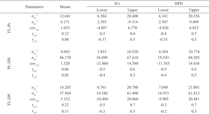
The bi-characteristics analyses in Table IV had posteriori means for the additive genetic variances and genetic correlation, residual and phenotypic with the credibility intervals and high-density region (all values were positive) for all three regions. The results in Table V indicate the values of heritability, credibility intervals and high-density regions.

The highest genetic variation of 37.629 was found in Diamante do Norte (DN), and the lowest of 6.244 was found in Palotina (PL) (Table II). Knowing that in both environments exist the same genetic representation, we can understand the greater genetic variation in DN environment as the environment that most favored the expression of the genetic potential of the animals. Rutten et al. (2005) reported an additive genetic variance from 1.481 to 2.778 from GIFT tilapia mated with other lines. Charo-Karisa et al. (2007) reported low estimates for additive genetic variation with weight of 782.8 g at the harvesting period. These results show the great genetic progress because of outstanding animals, and the genetic variation suggests continual weight gain (Ponzoni et al. 2005).

The differences in the “a posteriori” means for all of the parameters (Table II) were significant

TABLE II

Estimates of the variance components for live weight (g) from uni-characteristic analyses.

Site Parameters Means

ICr HPD

Lower Upper Lower Upper

PL

σa 2

6,244 2,616 9,203 2,790 9,350

σc 2

280 74 836 48 678

σw 2

241 76 580 51 502

σe 2

1,892 624 3,717 508 3,536

σy 2

8,657 6,553 10,720 6,508 10,650

FL

σa 2

13,679 6,454 20,500 6,281 20,245

σc 2

634 171 1,88 114 1,527

σw 2

585 169 1,594 114 1,329

σe 2

3,942 1,347 7,740 1,080 7,278

σy 2

18,841 14,26 24,040 14,053 23,801

DN

σ_a2

37,629 14,24 61,360 13,569 60,553

σc 2

1,519 418 4,524 289 3,679

σw 2

1,438 433 3,591 280 3,07

σe 2

14,968 4,237 27,420 3,736 26,653

σy 2

55,556 42,09 70,650 41,019 69,382

Credibility intervals (ICr) and high-density region (HPD),σ_a2

: additive genetic variance; σ_c2

: environmental variance common to larvae culture; σ_w2: environmental variance common to fingerlings; σ

e 2

: residual variance; σ_y2

: phenotypic variance.

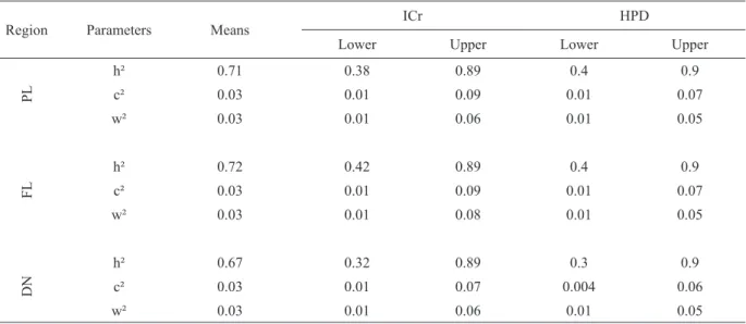
TABLE III

Heritability estimates (h²), participation of common environment of larvae culture (c²) and common environment of fingerlings (w²) in the phenotypic uni-characteristic analyses.

Region Parameters Means

ICr HPD

Lower Upper Lower Upper

PL

h² 0.71 0.38 0.89 0.4 0.9

c² 0.03 0.01 0.09 0.01 0.07

w² 0.03 0.01 0.06 0.01 0.05

FL

h² 0.72 0.42 0.89 0.4 0.9

c² 0.03 0.01 0.09 0.01 0.07

w² 0.03 0.01 0.08 0.01 0.05

DN

h² 0.67 0.32 0.89 0.3 0.9

c² 0.03 0.01 0.07 0.004 0.06

TABLE IV

Estimates from bi-characteristic analyses.

Parameters Means ICr HPD

Lower Upper Lower Upper

FL-PL

σa1 2

13.641 6.384 20.400 6.341 20.356

σa2 2

6.171 2.393 -9.314 2.507 9.409

cov_a12 1.035 -4.887 6.770 -4.826 6.823

r_a12 0.12 -0.5 0.6 -0.4 0.7

r_y12 0.08 -0.37 0.5 -0.35 0.5

PL-DN

σa1 2

8.065 3.855 10.530 4.304 10.774

σa3 2

46.170 18.490 67.610 19.243 68.205

cov_a13 1.320 -11.860 14.380 -11.765 14.436

r_a13 0.06 -0.5 0.6 -0.5 0.6

r_y13 0.05 -0.4 0.5 -0.4 0.5

FL-DN

σa2 2

14.203 6.761 20.780 7.048 21.001

σa3 2

37.564 14.180 61.490 14.553 61.813

cov_a23 5.152 -10.480 20.060 -9.905 20.481

r_a13 0.23 -0.5 0.7 -0.3 0.7

r_y13 0.11 -0.3 0.5 -0.2 0.5

Variance genetic: σa2

; covariance genetic: cov_a; genetic correlation: r_a; residual correlation: r_y; credibility intervals ICr and high density regions: HPD.

of treatment, care and water quality fertilizer tanks - when necessary).

In all of the environments, the participation of the common environment for fingerlings σ_c2,

280(PL), 634(FL), and 1,519(DN), and fingerlings σ_w2_{, 241(PL), 585(FL), and 1,438(DN), were}

similarly and relatively lower than reported by Santos et al. (2011), who found σ_c2 = 1,147.64 in

cage-nets where the common fingerling environment was a motherhood effect. The residual variation was

1,892(PL) and 3,942(FL), which were also lower

than the values reported by Santos et al. (2011), σe 2 ₌

5,965.53 in contrast to DN, where the variation was higher (14,968) than reported in the literature. The phenotypic variance among the regions, 8,657(PL), 18,841(FL) and 55,556(DN), and it performed similarly to the genetic (relatively low).

The “a posteriori” distribution of all parameters

was symmetric based on the closeness of the credibility interval and the high-density region. Because either the mean or the median could be

used to represent the distribution, the current option

was the mean “a posteriori”.

Based on the credibility intervals (Table II), we found residual heterogeneity of variance in the Palotina x Diamante environment and phenotypic heterogeneity variance in the Palotina x Floriano environment. Heterogeneity occurs when the credibility interval of a parameter in one region is not contained in the other region interval. In Table II, the Palotina interval (ICr = 624 – 3,717) is not contained in the ICr of Diamante do Norte (ICr = 4,237 – 27,420) and phenotypic heterogeneity of variance in Palotina (ICr = 6,553 – 10,720) x Diamante do Norte (ICr = 42,090 – 70,650) also exists as in Floriano (ICr = 14,260 – 24,040) x Diamante do Norte (ICr = 42,090 – 70,650) because of the genotype x environment interaction.

These heterogeneities can occur because the

differences in local management, stress, farming

sanitary conditions can affect the animal responses in every experimental condition. Variance differences

with subclass (regions) can reduce the accuracy of predicting parent values with an inadequate

selection of fish in different environments and can

consequently reduce the genetic progress (Weigel and Gianola 1993). Without residual heterogeneity, the results can overwhelm the data from animals raised in large environments.

The heritability values were higher from all of the regions (Table III) with 0.71 in Palotina, 0.72 in Floriano and 0.67 in Diamante do Norte of than authors working with previous generations, in this same lineage as presents Oliveira (2011) when the estimates of h² for live weight were 0.15 using Bayesian Inference and Santos et al. (2011), with a heritability of 0.39 for live weight at the harvesting time using frequentist inference. The increase in heritability results can be seen as a response to the selection that has occurred over the

years in this tilapia (fifth generation - G5) strain in

Paraná, which favors increased genetic and yield performance with each generation. Ponzoni et al. (2005) found h²=0.34 for live weight, similar to Nguyen et al. (2007), who reported an average of 0.35. The closest result to this current report was described by Charo-Karisa et al. (2006, 2007), who found a heritability of the live weight of 0.60 at harvesting time.

With high estimates of heritability, the emphasis of the selection must be centered at the individual level, which means that the best individuals are chosen as the reproducers. However, based on the average to low estimates of h2_{, the best choice is}

based on families. Individual selection exhibits fast responses in genetic gain/generation but the variability in small group is reduced in less time than the selection within the family.

Works with previous generations, show that participation in the genetic variation of the common

environment of larvae production and fingerlings

were close to zero, as reported by Oliveira (2011),

and lower than reported by Santos (2009) from

0.20 to 0.05 for σ_c2

(common maternal environment = common larvae production environment). The explanation for such high heritability values is that

of all of the fish participated in the genetic selection process and the current fifth generation and that

the selection criterion is daily weight gain highly correlated with live weight (0.99) (Porto et al. 2015).

The close estimates of the credibility intervals (ICr) and HPD confirm the symmetrical “a

posteriori” distributions (Table III). The small

interval of credibility for all of the parameters indicate high accuracy in the estimates. The bi-characteristic estimates are similar to the uni-characteristic estimates (Tables II and IV), thus strengthening all of the results of genotype x environment interaction (variance heterogeneity) and indicating that the uni-characteristic analyses are sufficient to explain the current genetic parameters.

environment, where the estimates from 0.58 to 0.65 were responses to this interaction. In Vietnam, the genetic correlation of weight at harvesting time from animals farmed in brackish and fresh water

was 0.45 (Luan et al. 2008).

A genetic correlation higher than 0.8 can discharge the genotype x environment correlation (Robertson 1959), but with estimates lower than

0.8-0.7, the fully genetic gain can only be achieved when the animals are selected and farmed in the same environment (Mulder et al. 2006) because a correlation lower than 0.7 indicates the presence of

interaction, as we found in the current experiment. The estimates from the uni-characteristic analyses were close to the bi-characteristic analyses

(Tables II and V), thus sustaining the results for high heritability. The credibility intervals for

bi-characteristic were lower, and they showed high precision in the results

The Spearman correlation from the uni-characteristic analysis was low (Table VI), where the highest was for Diamante do Norte x Floriano at 0.30 and the lowest was for Floriano x Diamante at 0.08. These values are lower than those reported by Santos (2009), who reported correlations from 0.75 to 0.84 (ground pound and cage-net) and 0.96 (cage net). The low values in the current experiment indicate interaction in the animal ranking. The same was observed with the genetic association from the Pearson correlation lower than 0.22 from Palotina x Diamante to 0.01 in Floriano x Diamante. These results indicate that after selecting animals from one region, they will not occupy the same rank in another location, which is strongly indicative of the interaction.

TABLE V

Estimates using the bi-characteristic analyses.

Regions Parameters Mean ICr

Lower Upper

FL-PL

h₁² 0.71 0.4 0.8

h₂² 0.70 0.3 0.8

c₁² 0.03 0.01 0.1

c₂² 0.03 0.01 0.1

w₁² 0.03 0.01 0.1

w₂² 0.03 0.01 0.1

PL-DN

h₁² 0.73 0.4 0.8

h₂² 0.66 0.3 0.8

c₁² 0.03 0.01 0.1

c₂² 0.03 0.01 0.1

w₁² 0.03 0.01 0.1

w₂² 0.03 0.01 0.1

FL-DN

h₂² 0.71 0.4 0.8

h₃² 0.70 0.3 0.8

c₂² 0.03 0.01 0.1

c₃² 0.03 0.01 0.1

w₂² 0.03 0.01 0.1

w₃² 0.03 0.01 0.1

TABLE VI

Spearman correlation above the diagonal and the Pearson below the diagonal from the uni-characteristic analyses.

Regions PL FL DN

PL 1 0.30 0.15

FL 0.16 1 0.08

DN 0.22 0.01 1

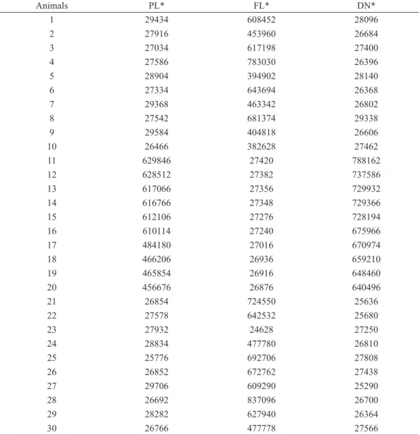
Based on the environment, the animal ranking

was modified, and no single species exhibited

similar records in all of the regions (Table VII). This fact also sustains the interaction for daily mean weight because of the numerous environmental factors such as weather conditions, management and farming systems.

Additional evidence of interaction was the direct gains with values higher than the indirect gains (Table VIII). This was the primary data obtained for

fish breeding because when farming occurs under similar selection conditions, the fish can reach their

TABLE VII

Fish ranking within the families based on high genetic values for live weight (g) from 1-10, intermediate genetic values from 11-20 and lower genetic values from 21-30 in the uni-characteristic analyses.

Animals PL* FL* DN*

1 29434 608452 28096

2 27916 453960 26684

3 27034 617198 27400

4 27586 783030 26396

5 28904 394902 28140

6 27334 643694 26368

7 29368 463342 26802

8 27542 681374 29338

9 29584 404818 26606

10 26466 382628 27462

11 629846 27420 788162

12 628512 27382 737586

13 617066 27356 729932

14 616766 27348 729366

15 612106 27276 728194

16 610114 27240 675966

17 484180 27016 670974

18 466206 26936 659210

19 465854 26916 648460

20 456676 26876 640496

21 26854 724550 25636

22 27578 642532 25680

23 27932 24628 27250

24 28834 477780 26810

25 25776 692706 27808

26 26852 672762 27438

27 29706 609290 25290

28 26692 837096 26700

29 28282 627940 26364

30 26766 477778 27566

full genetic potential with higher gains compared with farming in distinct environments. This result can guide future decisions about selection. Selecting cores and farming conditions in Brazil could intensify the results of breeding programs. Such decisions, however, require high initial investments that may hamper such work, but the incipient results (Table VIII) from the indirect selection show genetic gains because there were no situations with negative values, which indicate losses. In a situation where direct selection for weather and management is not possible, the indirect selection with lower genetic gains can increase productivity (Hulata 2001, Reis Neto et al. 2014).

The highest genetic gain was observed in Diamante do Norte (281.35 g/generation) (Table VIII) because previous generations were selected in net-cages and the cumulative genetic gain can

benefit the current generation with positive effects.

The values from Floriano (198.24 g/generation) and Palotina (98.74 g/generation) are distinct

because 100 g is a significant difference for two

similar ground pond environments. Therefore, this

difference may be the result of different management

approaches, such as feed quality, water quality, or

pond fertilization, which could affect the quantity of phytoplankton because tilapias are omnivorous filter fish that can use this resource when it is available.

TABLE VIII

Direct gain (g/selection generation) in the main diagonal and indirect gains (g/selection generation) above and

below this diagonal.

Gain PL FL DN

PL 98.74 16.38 16.43

FL 15.01 198.24 74.66

DN 7.77 38.52 281.35

The differences between Palotina and Floriano

were highlighted when the animals were selected in Diamante do Norte and evaluated in Palotina. The lower genetic gain of 7.77 g/generation was

incipient compared with the animals selected in Floriano and evaluated in Diamante do Norte, whose gains were 74.66 g/generation (Table VIII).

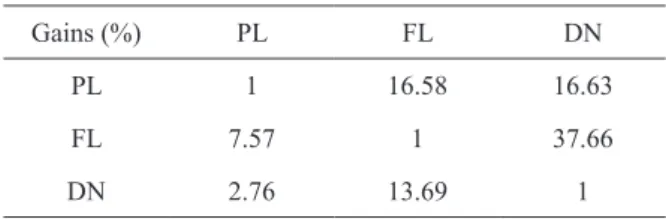
The low participation of indirect genetic gains on the direct ones is evidence of the interaction. The lower participation was in Diamante do Norte with Palotina, where the gain was 0.0276 g/generation, and the highest was 0.3766 g/generation in Floriano with Diamante do Norte (Table IX).

TABLE IX

Percentage of indirect participation in the direct gain in the three regions.

Gains (%) PL FL DN

PL 1 16.58 16.63

FL 7.57 1 37.66

DN 2.76 13.69 1

CONCLUSIONS

The evidence of the genotype x environment

interaction was verified by the results of the uni-

and bi-characteristic analyses, which indicated the phenotypic heterogeneity of the variances among

the three regions, weak genetic correlation, modified rankings in the different environments based on the

higher levels of direct genetic gains compared with indirect gains, and the lower participation (%) of the indirect gains in the direct gains. Such results

can guide further fish breeding programs.

REFERENCES

ABPA - ANUÁRIO BRASILEIRO DA PESCA E

AQUICULTURA. 2014. Florianópolis nº 1, ACEB, 135 p.

BAYE TM, ABEBE T AND WILKE RA. 2011. Genotype-environment interactions and their translational implications. NIH National Institute of Health, 2011 January 8(1): 59-70.

CERÓN-MUÑOZ MF, TONHATI H, COSTA CN, ROJAS-SARMIENTO D AND PORTILLA CS. 2004. Variance heterogeneity for milk yield in Brazilian and Colombian Holstein herds. LRRD 16: 1-8.

measurements, reproductive traits and gut length of Nile tilapia (Oreochromis niloticus) selected for growth in low-input earthen ponds. Aquaculture 273: 15-23. CHARO-KARISA H, KOMEN H, REZK MA, PONZONI

RW, VAN AJ AND BOVENHUIS H. 2006. Heritability estimates and response to selection for growth of Nile tilapia (Oreochromis niloticus) in low-input earthen ponds. Aquaculture 261: 479-486.

EKANATH AE, BENTSEN HB, PONZONI RW, RYE M, NGUIYEN NH, THODESEN J AND GJERDE B. 2007. Genetic improvement of farmed tilapias: Composition and genetic parameters of a synthetic base population of

Oreochromis niloticus for selective breeding. Aquaculture 273: 1-14.

HEIDELBERG P AND WELCH PD. 1983. Simulation Run Length Control in the Presence of an Initial Transient. Oper Res 31: 1109-1144.

HILSDORF AWS, PERAZZA CA, MOREIRA HLM AND FREITAS RTF. 2014. Como fazer melhoramento genético em sua piscicultura: As bases para o melhoramento genético por seleção individual em médias propriedades. Panor Aquic 133: 34 -36.

HULATA G. 2001. Genetic manipulation in aquaculture: a review of stock improvement by classical and modern technologies. Genetica 111: 155-173.

IBGE - INSTITUTO BRASILEIRO DE GEOGRAFIA E ESTATISTICA. 2014. Sistema IBGE de Recuperação Automática, Sidra, Tabela 3940, Produção da aquicultura por tipo de produto. Disponível em <http://www.sidra. ibge.gov.br/bda/ tabela/listabl.asp?c=3940&n=0&z= t&o=21&i=P>. Acesso em: 09 set. 2015.

KHAW HL, BOVENHUIS H, PONZONI RW, REZK MA, CHARO-KARISA H AND KOMEN H. 2009b. Genetic analysis of Nile tilapia (Oreochromis niloticus) selection line reared in two input environments. Aquaculture 294: 37-42. K H AW H L , P O N Z O N I RW, H A M Z A H A A N D

K A M A R U Z Z A M A N N . 2 0 0 9 a . G e n o t y p e b y environmental interaction for live weight between two production environments in the GIFT strain (Nile tilapia,

Oreochromis niloticus). Proc Assoc Advmt Anim Breed Genet 18: 60-63a.

LUAN TD, OLESEM I, ODEGARD J, KOLSTAD K AND DAN NC. 2008. Genotype by environment interaction for harvest body weight and survival of Nile tilapia (Oreochromis niloticus) in brackish and fresh water ponds. 8th

International Symposium on Tilapia in Aquaculture, 12, 2008. Cairo, Egypt. Proceeding, 231 p.

LUPCHINSKI JE, VARGAS L, POVH JA, RIBEIRO RP, MANGOLIM CA AND LOPERA BARRERO NM. 2008. Avaliação da variabilidade das gerações G0 e F1 da linhagem GIFT de tilápia-do-nilo (Oreochromis niloticus) por RAPD. Acta Sci Anim Scie 30: 233-240.

MULDER HA, VEERKAMP RF, DUCRO BJ, VAN AJA AND BIJMA P. 2006. Optimization of dairy cattle breeding programs for different environment with genotype by environment interaction. J Dairy Sci 89: 1740-1752. NGUYEN NH, KHAW HL, PONZONI RW, HAMZAH

A AND KAMARUZZAMAN N. 2007. Can sexual dimorphism and body shape be altered in Nile tilapia (Oreochromis niloticus) by genetic means? Aquaculture 272: S38-S46.

OECD/FAO - ORGANIZAÇÃO PARA COOPERAÇÃO E D E S E N V O LV I M E N T O E C O N Ô M I C O / ORGANIZAÇÃO DAS NAÇÕES UNIDAS PARA ALIMENTAÇÃO E AGRICULTURA. 2015. OECD-FAO Agricultural Outlook 2015, Paris: OECD Publishing, 145 p. Disponível em: <http://www.oecd-ilibrary.org/ agriculture-and-food/oecd-fao-agricultural-outlook-2015_ agr_outlook-2015-en>. Acesso em: 05 out. 2015. DOI: http://dx.doi.org/10.1787/agr_outlook-2015-en.

OLIVEIRA SN. 2011. Parâmetros genéticos para características de desempenho e morfométricas em tilápias do Nilo (Oreochromis niloticus). 39 p. Dissertação de Mestrado - Universidade Estadual de Maringá, Maringá. (Unpublished).

P O N Z O N I RW, H A M Z A H A , TA N S A N D KAMARUZZAMAN N. 2005. Genetic parameters and response for live weight in the GIFT strain of Nile tilapia (Oreochromis niloticus). Aquaculture 247: 203-210. PONZONI RW, NGUYEN NH, KHAW HL AND NINH NH.

2008. Accounting for genotype by environment interaction in economic appraisal of genetic improvement programs in common carp Cyprinus carpio. Aquaculture 285: 47-55. PORTO EP, OLIVEIRA ACL, MARTINS EN, RIBEIRO

RP, CONTI ACM, KUNITA NM, OLIVEIRA SN AND PORTO PP. 2015. Respostas à seleção de características de desempenho em tilápia-do-nilo. Pesqui Agropecu Bras 50(9): 9.

REIS NETO RV, OLIVEIRA CAL, RIBEIRO RP, FREITAS RTF, ALLAMAN IV AND OLIVEIRA SN. 2014. Genetic parameters and trends of morphometric traits of GIFT tilapia under selection for weight gain. Sci Agric 71: 259-265. RESENDE MDV. 2007. Matemática e estatística na análise

de experimentos e no melhoramento genético. Brasília: Embrapa Florestas, Brasilia, Brazil, 362 p.

ROBERTSON A. 1959. The sampling variance of the genetic correlation coefficient. Biometrics 15: 469.

RODRIGUES FIFLHO M, ZANGERONIMO MG, LOPES LS, LADEIRA MM AND ANDRADE I. 2011. Fisiologia do crescimento e desenvolvimento do tecido muscular e sua relação com a qualidade da carne em bovinos. Revista Eletrônica Nutritime 8(2): 1431-1443.

genetic parameters for body weight and survival of Nile tilapia farmed in Brazil. Pesqui Agropecu Bras 46: 33-43.

SANTOS AI. 2009. Interação genótipo-ambiente e estimativas

de parâmetros genéticos em Tilápias (Oreochromis niloticus). 85 p. Dissertação de Doutorado - Universidade Estadual de Maringá, Maringá. (Unpublished).

SAS INSTITUTE. 2000. User’s guide: statistics, version 8.1.4. v.2. Cary: SAS Institute.

VAN TASSEL CP AND VAN VLECK LD. 1995. A manual for the use of MTGSAM: A set of FORTRAN programs to apply Gibbs sampling to animal models for variance component estimation (Draft). Lincon: Department of Agriculture/Agricultural Research Service.