Low-rise structures in reinforced concrete: approximation of material nonlinearity for global stability analysis

(1)

Low-rise structures in reinforced concrete:

approximation of material nonlinearity for global

stability analysis

Estruturas de pequeno porte em concreto armado:

consideração aproximada da não-linearidade física para

análise da estabilidade global

a _{Federal Institute of Education, Science and Technology of Mato Grosso do Sul, Department of Infrastructure, Aquidauana, MS, Brazil;} b _{State University of Maringá, Department of Civil Engineering, Maringá, PR, Brazil.}

Received: 08 Dec 2016 • Accepted: 06 Feb 2017 • Available Online: 15 Feb 2018

L. M. MOREIRA a

[email protected] C. H. MARTINS b

[email protected]

Abstract

Resumo

In the analysis of the second-order global effects, the material nonlinearity (NLF) can be considered in an approximate way, defining for the set of each structural element a mean flexural stiffness. However, there is less research concerning low-rise buildings in the analysis of global stabil -ity in contrast to high buildings, because these have a greater sensitiv-ity to this phenomenon and they are more studied. In this way, the paper objective is to determine the flexural stiffness values, of beams and columns, for buildings with less than four floors, to approximate consideration of the NLF in the global analysis. The idealized examples to buildings with 1, 2 and 3 floors, being simulated through the software CAD/TQS and an analysis model based in an iterative process. The simulations results defined the stiffness values of the set of beams and columns in each example, followed by a statistical analysis to define general values of application in the buildings. Finally, a proposal is suggested of stiffness reduction coefficients for beams and columns to be adopted in the approximation the NLF (EI_sec= α_v/p∙ E_ci I_c), as follows: buildings with 1 floor (α_v= 0,17 and α_p= 0,66), buildings with 2 floors (α_v= 0,15 and α_v= 0,71) and buildings with 3 floors (α_v= 0,14 and α_v= 0,72). The results obtained can be used for the analysis of low-rise structures to consider the second order global effects with more safely.

Keywords: second order effects, global analysis, stiffness of structural elements.

Na análise dos efeitos globais de segunda ordem, a não-linearidade física (NLF) pode ser considerada de forma aproximada, definindo-se para o conjunto de cada elemento estrutural, uma rigidez secante à flexão. No entanto, encontram-se menos pesquisas referentes a edifícios baixos na análise da estabilidade global em contraste com os edifícios altos, pois estes possuem uma maior sensibilidade a esse fenômeno e, consequen-temente, são objeto de maior estudo. Desta forma, o objetivo deste trabalho é determinar os valores de rigidez à flexão, de vigas e pilares, para edificações com menos de quatro pavimentos, de modo a considerar a NLF de forma aproximada na análise global. Os exemplos idealizados são referentes a edificações com 1, 2 e 3 pavimentos, sendo simulados através do software CAD/TQS e por meio de um modelo de análise baseado em um processo iterativo. Os resultados das simulações definiram os valores da rigidez do conjunto de vigas e de pilares em cada exemplo, prosseguindo-se a uma análise estatística com o intuito de se definir valores gerais de aplicação nas edificações. Por fim, apresenta --se uma proposta de coeficientes redutores de rigidez para vigas e pilares a serem adotados na consideração da NLF de forma aproximada (EI_sec= α_v/p∙ E_ci I_c), conforme a seguir: edifícios com 1 pavimento (α_v= 0,17 e α_p= 0,66), edifícios com 2 pavimentos (α_v= 0,15 e α_v= 0,71) e edifícios com 3 pavimentos (α_v= 0,14 e α_v= 0,72). Os resultados obtidos podem ser utilizados para a análise de estruturas de pequeno porte de modo a se considerar os efeitos globais de segunda ordem de forma mais segura.

(2)

1. Introduction

Basically, a global stability analysis evaluates the global second-order effects on buildings, considering the material nonlinearity of the included materials and the geometric nonlinearity that result from the structure in its deformed state. However, at that stage, the struc-tural elements are not yet scaled out, and consequently, there are no details on the armor. As a result, the global stability analysis is char-acterized as a preliminary step before scaling structures, and thus, an approximate evaluation of the material nonlinearity is conducted. The material nonlinearity can be approximately considered, by es-tablishing the secant stiffness of bending for each structural ele-ment. However, there have been very few studies on low rise build-ings in the analysis of global stability compared to tall buildbuild-ings because these have a higher sensitivity to this phenomenon, and consequently, are subject to more studies.

This idea is corroborated by the fact that the ABNT NBR 6118:2014 in its item 15.7.3 proposes approximate stiffness values for beams, columns and slabs in buildings with at least four floors.

According to IBRACON (2015), the use of these stiffness values proposed by the standards organization for smaller buildings may lead to results detrimental to the safety of the structures as these values are usually smaller.

However, setting the stiffness for the entire set of beams and col-umns in low rise buildings is essential but highly complex at the same time. In fact, each building has unique features that, in turn, affect the setting of the secant stiffness of the entire set of its struc -tural elements. Thus, statistical analysis becomes an important tool for the integration of the specificities of each building.

Khuntia and Ghosh (2004a) obtained values of effective bending stiff-ness (

EI

_ef) for beams and columns through an analytical approach. They conducted a parametric study where the analysis of beams and columns was conducted separately to investigate the dependency that exists between bending stiffness and other relevant parameters. According to the results obtained, they proposed an equation for the calculation of

EI

_ef for columns, by equation 1.

(1)

where:

EI_ef: effective bending stiffness;

E_cI_g: bending stiffness of the gross section;

ρg : longitudinal armor rate;

e ⁄ h : relative eccentricity;

ρu : requested normal force of calculation; ρ0 : resistant normal force of calculation.

For beams, they proposed expressions for the following situations:

I. For rectangular beams with

f

ck

≤

41, 4 MPa

, the

EI

ef can be

calculated by equation 2 or equation 3 that consider the inertia moment of the cracked section.

(2)

(3)

where

ρg : longitudinal armor rate;

b : width of the beam; d : clear height of the section; c : depth of the neutral line;

n : relationship between the elasticity modules of steel and concrete; A_s: positive armature steel area.

II. For rectangular beams with

f

ck

>

41, 4

MPa

, the

EI

ef can be

calculated by equation 4.

(4)

where:

ρ_g: longitudinal armor rate; b : width of the beam; d : clear height of the section; f_c' : concrete’s compressive strength.

III. For beams with section T and compressed table, the

EI

ef can

be calculated by equation 5.

(5)

where

EI_efT : effective bending stiffness for beams with T-section; EI_ef : effective bending stiffness for rectangular beams; t_f : width of the table;

h: height of the section.

Based on the equations, Khuntia and Ghosh (2004a) suggested a methodology for considering the values of

EI

_ef for portico beams and columns, with emphasis on slender columns:

1. In the analysis of porticos, for the consideration of the global effects of first and second-order, values of EIef = 0,35 ∙ EcIg for

beams and EI_ef= 0,7 ∙ E_cI_g for columns can be assumed. 2. At the end of this first analysis, the values of EI_ef for the beams

and columns were recalculated following equations 1 and 2. If the values obtained are greater than 15% of the initial values considered, it is recommended to perform a new analysis using the values obtained by the equations. Otherwise, performing a new analysis is not required.

Khuntia and Ghosh (2004b) validated the analytic approach designed in Khuntia and Ghosh (2004a) through experimental analysis. Martins (2008) analyzed reinforced concrete beams, bi-supported and bi-embedded, with different rates of longitudinal armor and distributed loads, using a finite element formulation, considering integrated concrete between cracks as a contributing factor

(ten-sion stiffening) and M-1/r diagrams to evaluate the

EI

ef of the

beams in the two above-mentioned binding situations. For the bi-supported beams, the values obtained were 0,41 ∙ EciIc ≤ EIef ≤

0,54 ∙ Eci Ic. For the bi-embedded beams, the values obtained were

0,57 ∙ EciIc ≤ EIef ≤ 0,64 ∙ EciIc, where

E

ci is the concrete’s initial

(3)

reinforced concrete buildings should be an intermediate situation in relation to those analyzed, the approximate

EI

_ef for the beams should be considered as 0,54 ∙ EciIc in verifications of the ultimate

state limit design. However, according to the results obtained, Martins emphasized that the

EI

_ef should be differentiated for the

beams with equal and different lower and upper armor.

The ACI 318:2014 suggests the use of equations 1 and 2 pro-posed by Khuntia and Ghosh (2004a) for the calculation of

EI

ef

for columns and beams, respectively. However, for the columns, the limits of 0,35 ∙ EcIg ≤ EIef ≤ 0,875 ∙ EcIg are set. Moreover, for the

beams, the limits are 0,25 ∙ EcIg ≤ EIef ≤ 0,50 ∙ EcIg. The final values

of

EI

_ef should also be multiplied by the reduction factor ∅_k= 0,875. According to Franco (1995), this reduction only makes sense for the general formulation of the American standard.

Bueno (2014) determined stiffness values to be used for beams (EI_sec = α_v ∙ E_ciI_c) and columns (EI_sec = α_p ∙ E_ciI_c) in buildings with less than four floors, to consider the material nonlinearity, in an approximate manner, in the evaluation of global stability. To obtain these values, a number of examples were designed and their re-spective analyses were conducted using the CAD/TQS software, version 16.9.79, considering the specifications of the ABNT NBR 6118:2007. Finally, the following values for the stiffness coefficients were suggested: buildings with 1 floor (αv = 0,20 and αp = 0,60),

buildings with 2 floors (αv = 0,30 and αp = 0,60), buildings with

3 floors (α_v= 0,30 and α_p = 0,70) and buildings with 4 to 10 floors (α_v= 0,40 and α_p = 0,80).

As defined earlier, in the global analysis, the geometric nonlinearity is associated with the changes that occur in the geometry of the structure as a whole and there are established methods to evalu-ate it (e. g., coefficient γ_z, P-Δ analysis, the method of the geometric stiffness matrix). However, the consideration of the geometric non-linearity essentially depends on a good evaluation of the deformed structure, i.e., the correct consideration of the material nonlinearity.

1.1 Objective

To determine the values of bending stiffness of beams and col-umns, for buildings with less than four floors; to enable the evalu-ation of material nonlinearity, in an approximate manner, for the global stability analysis of low rise buildings.

1.2 Justification

The ABNT NBR 6118:2014 suggests the use of the instability parameter α and/or the coefficient γ_z for the evaluation of global second-order effects.

Unlike the instability parameter α that incorporates the values of bending stiffness of the cross-linked structure in its formulation, it becomes necessary to consider the material nonlinearity with stiff-ness reducing values of the structural elements suggested by the standard in item 15.7.3 in the calculation of the coefficient γz.

How-ever, these values are for buildings with at least four floors, thus preventing the use of the coefficient γz in smaller buildings.

Because the instability parameter α does not have this limitation, it can be used to assess the overall stability instead of the coefficient

γ_z. However, the instability parameter α does not allow the calcula-tion of the second-order global effects, unlike the coefficient γ_z.

Therefore, the determination of the stiffness values of structural elements for buildings with less than four floors makes it possible to use the coefficient γz for the evaluation of global stability and

calculation of the second-order global effects (when needed) for buildings of this size.

In relation to the calculation of the second-order global effects, the values of bending stiffness can also be used in considerably com-plex methods for the evaluation of geometric nonlinearity, such as the P-Δ analysis and the geometric stiffness matrix method.

2. Materials and numerical simulations

In this study, we attempted to define an analysis method different from that employed by Bueno (2014), to expand the investigation of the approximate material nonlinearity into the evaluation of glob-al stability. According the objective, it is required to set the stiffness values of beams (EI_sec = α_v ∙ E_ciI_c) and columns (EI_sec = α_p ∙ E_ciI_c) for buildings with less than four floors.

As such, we used the CAD/TQS software, version 18.11.53, made available by the Department of Civil Engineering of the State Univer-sity of Maringa, because it fulfills the requirements of the ABNT NBR 6118:2014 and includes advanced and automated analysis methods.

2.1 Characterization of the studied examples

The examples studied are relative to buildings with one, two, and three floors. The following are some fixed characteristics adopted in all examples:

n For the classification of environmental aggressiveness, we se-lected class II;

n The presence of masonry walls was considered over all the beams on all floors (on the coverage floors, the height of the walls was of 1 m), composed of concrete blocks 14 and 19 cm wide for beams 15 and 20 cm wide, respectively;

n The slabs of the standard pavement are 12 cm thick with 2.0

and 3.0 kN/m² permanent and accidental load, respectively.

Figure 1

Plant of structural shapes T

₁

(4)

While the slabs of the coverage pavement are 12 cm thick with 3.0 ken/m² of permanent and incidental load;

n The action of the wind and geometric imperfections in four di-rections (0°, 90°, 180° and 270°) were also taken into consider-ation, resulting in 83 combinations of actions for analysis. For the analysis of the size of each building 16 examples were designed, based on different types of structural shapes, structural configurations, basic wind speeds and characteristic strength of concrete. These param-eters are presented in Figures 1 and 2 and Tables 1, 2 and 3.

It should be noted that, from the structural configurations listed in Table 1, only classifications E and F are used in the examples with three floors. Classifications G and H are only used in the examples with two floors. Classifications I and J are only used in the examples with one floor. This differentiation was used to

es-Figure 2

Plant of structural shapes T

₂

Source: Author

Table 1

Types of structural configurations

Nomenclature Beams

(cm x cm)

Columns (cm x cm)

Height of floor to floor (m)

Length of beams (m)

E 20 x 50 20 x 50 4 5

F 20 x 40 20 x 40 3 4

G 20 x 40 20 x 40 4 5

H 15 x 40 15 x 40 3 4

I 20 x 40 20 x 35 4 5

J 15 x 30 15 x 25 3 4

Source: Author

Table 2

Types of basic wind speed (V

₀

)

Nomenclature Basic wind speed (m/s)

v1 30

v₂ 50

Source: Author

Table 3

Types of characteristic strength of concrete (f

_ck

)

Nomenclature Characteristic strength of concrete (MPa)

f 25

g 40

Source: Author

Table 4

Examples for simulations

Combinations

3T₁Ev₁f 3T₁Ev₁g 3T₁Ev₂f 3T₁Ev₂g

3T₁Fv₁f 3T₁Fv₁g 3T₁Fv₂f 3T₁Fv₂g

3T₂Ev₁f 3T₂Ev₁g 3T₂Ev₂f 3T₂Ev₂g

3T₂Fv₁f 3T₂Fv₁g 3T₂Fv₂f 3T₂Fv₂g

2T₁Gv₁f 2T₁Gv₁g 2T₁Gv₂f 2T₁Gv₂g

2T₁Hv₁f 2T₁Hv₁g 2T₁Hv₂f 2T₁Hv₂g

2T₂Gv₁f 2T₂Gv₁g 2T₂Gv₂f 2T₂Gv₂g

2T₂Hv₁f 2T₂Hv₁g 2T₂Hv₂f 2T₂Hv₂g

1T₁Iv₁f 1T₁Iv₁g 1T₁Iv₂f 1T₁Iv₂g

1T₁Jv₁f 1T₁Jv₁g 1T₁Jv₂f 1T₁Jv₂g

1T₂Iv₁f 1T₂Iv₁g 1T₂Iv₂f 1T₂Iv₂g

1T₂Jv₁f 1T₂Jv₁g 1T₂Jv₂f 1T₂Jv₂g

(5)

timate the features compatible with those used in real buildings. Thus, Table 4 shows the list of simulated examples. The symbols used are listed in Table 5.

The variability used in designing the examples was adopted to ob-tain different detailing of the armor in the structural elements, and consequently, different rates of longitudinal armor. It should also be considered that the stiffness of structural elements is sensitive to the variation of the steel rate set for each structural element.

2.2 Analysis of model examples

Having defined the examples, the next step is to demonstrate their

analysis. The analysis model is developed based on an iterative process to obtain the results, where, after the convergence, the av-erage stiffness values obtained for beams and columns accurately represent the material nonlinearity, in an approximate manner, for the simulated example.

Figure 3 shows the simulation process of all examples on a flowchart.

2.2.1 Processing 1

Initially, the material nonlinearity is evaluated, approximately, with the values of stiffness for the beams (EIsec = 0,4 ∙ EciIc) and the columns

(EI_sec = 0,8 ∙ E_ciI_c) — note that although these values are common for

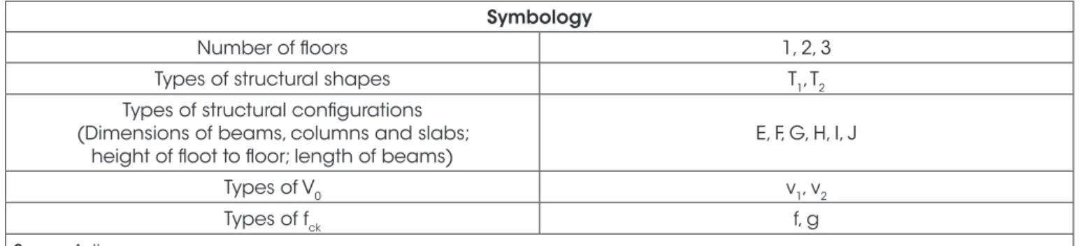
Table 5

Description of symbology adopted in table 4

Symbology

Number of floors 1, 2, 3

Types of structural shapes T₁, T₂

Types of structural configurations (Dimensions of beams, columns and slabs;

height of floot to floor; length of beams)

E, F, G, H, I, J

Types of V₀ v₁, v₂

Types of f_ck f, g

Source: Author

Figure 3

Analysis model of examples

(6)

buildings with four or more floors, they were used as an initial mea-sure. The geometric nonlinearity is analyzed by the P-Δ analysis. After the estimation of global effects (1st_{order + 2}nd order), we continue

with the analysis of the local effects of second-order on the columns. As such, after setting the value of the total effects in each element, the dimensioning and detailing of structural elements is done, ac-cording to the parameters defined in the ABNT NBR 6118:2014.

2.2.2 Processing 2

On the basis of the material and geometric nonlinear portico the

material nonlinearity is evaluated by M-1/r and N-M-1/r diagrams,

for beams and columns, respectively. Analogous to processing 1, the geometric nonlinearity is evaluated by the P-Δ analysis. This processing consists of only one verification with respect to the ultimate state limit design and provides the stiffness values for each bar element discretized from the beams and columns. Such discretization is made for 50 cm long bar elements, as a simi-lar performance is evident in preliminary tests for the discretization of 10 cm long bar elements. With respect to the savings on compu-tational costs, the choice was justified.

For discretized bars that do not comply with the ultimate state limit

Table 6

Results of the simulations (part 1)

Example 1ª iteration 2ª iteration 3ª iteration 4ª iteration 5ª iteration Estimated Average rate of beams armor (%) Average rate of columns armor (%)

3T1Ev1f αv:0,16

α_p:0,75

α_v:0,15 α_p:0,72

α_v:0,15 α_p:0,71

α_v:0,15

α_p:0,72

-α_v:0,15

α_p:0,72 0,92 0,73

3T1Ev1g αv:0,13

α_p:0,79

α_v:0,12 α_p:0,74

α_v:0,12

α_p:0,74 -

-α_v:0,12

α_p:0,74 0,83 0,5

3T1Ev2f αv:0,16

α_p:0,74

α_v:0,15 α_p:0,71

α_v:0,15

α_p:0,71 -

-α_v:0,15

α_p:0,71 0,92 0,76

3T1Ev2g αv:0,13

α_p:0,79

α_v:0,13 α_p:0,74

α_v:0,13

α_p:0,74 -

-α_v:0,13

α_p:0,74 0,92 0,5

3T1Fv1f αv:0,14

α_p:0,77

α_v:0,15 α_p:0,73

α_v:0,15

α_p:0,73 -

-α_v:0,15

α_p:0,73 0,75 0,59

3T1Fv1g αv:0,11

α_p:0,82

α_v:0,13 α_p:0,77

α_v:0,13

α_p:0,77 -

-α_v:0,13

α_p:0,77 0,69 0,59

3T1Fv2f αv:0,14

α_p:0,77

α_v:0,16 α_p:0,73

α_v:0,15 α_p:0,73

α_v:0,15

α_p:0,73

-α_v:0,15

α_p:0,73 0,8 0,6

3T1Fv2g αv:0,11

α_p:0,82

α_v:0,13 α_p:0,77

α_v:0,13

α_p:0,77 -

-α_v:0,13

α_p:0,77 0,72 0,59

3T2Ev1f αv:0,18

α_p:0,74

α_v:0,15 α_p:0,69

α_v:0,15 α_p:0,68

α_v:0,15

α_p:0,68

-α_v:0,15

α_p:0,68 0,85 0,62

3T2Ev1g αv:0,15

α_p:0,78

α_v:0,12 α_p:0,72

α_v:0,12 α_p:0,71

α_v:0,12

α_p:0,71

-α_v:0,12

α_p:0,71 0,82 0,5

3T2Ev2f αv:0,20

α_p:0,72

α_v:0,16 α_p:0,68

α_v:0,16

α_p:0,68 -

-α_v:0,16

α_p:0,68 1,03 0,83

3T2Ev2g αv:0,17

α_p:0,76

α_v:0,13 α_p:0,70

α_v:0,13

α_p:0,70 -

-α_v:0,13

α_p:0,70 0,96 0,56

3T2Fv1f αv:0,14

α_p:0,75

α_v:0,15 α_p:0,70

α_v:0,15

α_p:0,70 -

-α_v:0,15

α_p:0,70 0,72 0,6

3T2Fv1g αv:0,11

α_p:0,80

α_v:0,13 α_p:0,73

α_v:0,13 α_p:0,74

α_v:0,13

α_p:0,74

-α_v:0,13

α_p:0,74 0,68 0,59

3T2Fv2f αv:0,14

α_p:0,75

α_v:0,16 α_p:0,69

α_v:0,16 α_p:0,70

α_v:0,16

α_p:0,70

-α_v:0,16

α_p:0,70 0,76 0,6

3T2Fv2g αv:0,12

α_p:0,79

α_v:0,14 α_p:0,72

α_v:0,14 α_p:0,73

α_v:0,14

α_p:0,73

-α_v:0,14

α_p:0,73 0,72 0,59

(7)

design, minimum increases are manually made in the respective areas of longitudinal armor and, then, the example undergoes an-other analysis with respect to material nonlinearity and geomet-ric nonlinearity by means of the material and geometgeomet-ric nonlinear portico, obtaining new values of stiffness for each discretized bar. This process is repeated until all the elements comply with ultimate state limit design.

Subsequently, a note is made on the average values of stiffness provided by the software, for the whole set of beams and columns of the structure.

2.2.3 Iterative process

We replace the initial values of material nonlinearity (beams: EI_sec = 0,4 ∙ E_ciI_c and columns: EI_sec = 0,8 ∙ E_ciI_c) with the obtained co-efficients (average values of stiffness) and repeat processing 1 and 2. As the values of the coefficients are presented with an accuracy of two decimal places, this iterative process is repeated until the values of an iteration are equal to those of a previous iteration. After convergence, the obtained values represent the evaluation of

the material nonlinearity, in an approximate manner, for that structure.

Table 6

Results of the simulations (part 2)

2T1Gv1f αv:0,18

α_p:0,70

α_v:0,18 α_p:0,69

α_v:0,18

α_p:0,69 -

-α_v:0,18

α_p:0,69 1,34 0,85

2T1Gv1g αv:0,15

α_p:0,74

α_v:0,15 α_p:0,71

α_v:0,15

α_p:0,71 -

-α_v:0,15

α_p:0,71 1,26 0,7

2T1Gv2f αv:0,18

α_p:0,70

α_v:0,18 α_p:0,69

α_v:0,18

α_p:0,69 -

-α_v:0,18

α_p:0,69 1,28 0,87

2T1Gv2g αv:0,15

α_p:0,75

α_v:0,14 α_p:0,72

α_v:0,14

α_p:0,72 -

-α_v:0,14

α_p:0,72 1,24 0,74

2T1Hv1f αv:0,15

α_p:0,81

α_v:0,16 α_p:0,76

α_v:0,15 α_p:0,76

α_v:0,15

α_p:0,76

-α_v:0,15

α_p:0,76 0,81 1,03

2T1Hv1g αv:0,13

α_p:0,84

α_v:0,14 α_p:0,78

α_v:0,13 α_p:0,78

α_v:0,14

α_p:0,78

-α_v:0,14

α_p:0,78 0,81 0,79

2T1Hv2f αv:0,15

α_p:0,82

α_v:0,15 α_p:0,76

α_v:0,15

α_p:0,76 -

-α_v:0,15

α_p:0,76 0,79 1,01

2T1Hv2g αv:0,13

α_p:0,85

α_v:0,14 α_p:0,78

α_v:0,13 α_p:0,79

α_v:0,14

α_p:0,78

-α_v:0,14

α_p:0,78 0,83 0,79

2T2Gv1f αv:0,18

α_p:0,68

α_v:0,18 α_p:0,65

α_v:0,18

α_p:0,65 -

-α_v:0,18

α_p:0,65 1,27 0,76

2T2Gv1g αv:0,15

α_p:0,72

α_v:0,15 α_p:0,67

α_v:0,15

α_p:0,67 -

-α_v:0,15

α_p:0,67 1,17 0,66

2T2Gv2f αv:0,19

α_p:0,67

α_v:0,18 α_p:0,65

α_v:0,19 α_p:0,64

α_v:0,18

α_p:0,65

-α_v:0,18

α_p:0,65 1,31 0,88

2T2Gv2g αv:0,15

α_p:0,70

α_v:0,15 α_p:0,66

α_v:0,15

α_p:0,66 -

-α_v:0,15

α_p:0,66 1,26 0,78

2T2Hv1f αv:0,16

α_p:0,80

α_v:0,16 α_p:0,73

α_v:0,16

α_p:0,73 -

-α_v:0,16

α_p:0,73 0,8 0,93

2T2Hv1g αv:0,14

α_p:0,82

α_v:0,14 α_p:0,75

α_v:0,14

α_p:0,75 -

-α_v:0,14

α_p:0,75 0,73 0,79

2T2Hv2g αv:0,14

α_p:0,81

α_v:0,14 α_p:0,73

α_v:0,14

α_p:0,73 -

-α_v:0,14

α_p:0,73 0,76 0,79

1T1Iv1f αv:0,19

α_p:0,68

α_v:0,17 α_p:0,64

α_v:0,17 α_p:0,65

α_v:0,17

α_p:0,65

-α_v:0,17

α_p:0,65 1,06 0,46

(8)

2.3 Statistical treatment

With the stiffness values estimated in each example owing to the iterative process, one should perform the statistical treatment to obtain the average values of the stiffness reducing coefficients for evaluation of the material nonlinearity, in an approximate manner, for buildings with one, two and three floors.

Thus, the measures used to describe the set of values obtained in each example are measures of central tendency (representa-tive average) and measures of dispersion (standard deviation, coefficient of variation, and maximum and minimum values). We also used Gaussian distribution graph x histogram, to compare the distribution mathematically established with the one that

represents the numerically obtained data.

The representative average is the value that the data of a distribu-tion concentrates the most and, for the purpose of this study, it can be defined by equation 6.

(6)

where

n: number of simulated examples;

α_(v/p):average stiffness reduction coefficient of beams or columns;

α(v/p)i : stiffness reducing coefficient of the beams or columns,

ob-tained in each example.

The standard deviation represents the variation or dispersion that

Table 6

Results of the simulations (part 2)

1T1Iv1g αv:0,16

α_p:0,71

α_v:0,14 α_p:0,64

α_v:0,14

α_p:0,64 -

-α_v:0,14

α_p:0,64 1,12 0,73

1T1Iv2f αv:0,19

α_p:0,67

α_v:0,17 α_p:0,65

α_v:0,17 α_p:0,64

α_v:0,17

α_p:0,64

-α_v:0,17

α_p:0,64 1,09 0,8

1T1Iv2g αv:0,16

α_p:0,71

α_v:0,14 α_p:0,65

α_v:0,14 α_p:0,64

α_v:0,14

α_p:0,64

-α_v:0,14

α_p:0,64 1,07 0,73

1T1Jv1f αv:0,17

α_p:0,76

α_v:0,19 α_p:0,73

α_v:0,19

α_p:0,73 -

-α_v:0,19

α_p:0,73 1,27 1,42

1T1Jv1g αv:0,14

α_p:0,78

α_v:0,15 α_p:0,73

α_v:0,15

α_p:0,73 -

-α_v:0,15

α_p:0,73 1,12 1,25

1T1Jv2f αv:0,17

α_p:0,75

α_v:0,19 α_p:0,73

α_v:0,19

α_p:0,73 -

-α_v:0,19

α_p:0,73 1,25 1,55

1T1Jv2g αv:0,14

α_p:0,78

α_v:0,15 α_p:0,73

α_v:0,15

α_p:0,73 -

-α_v:0,15

α_p:0,73 1,12 1,29

1T2Iv1f αv:0,21

α_p:0,67

α_v:0,19 α_p:0,62

α_v:0,19

α_p:0,62 -

-α_v:0,19

α_p:0,62 1,11 0,56

1T2Iv1g αv:0,18

α_p:0,71

α_v:0,15 α_p:0,63

α_v:0,15 α_p:0,62

α_v:0,15

α_p:0,62

-α_v:0,15

α_p:0,62 1,03 0,56

1T2Iv2f αv:0,21

α_p:0,66

α_v:0,19 α_p:0,62

α_v:0,19

α_p:0,62 -

-α_v:0,19

α_p:0,62 1,05 0,59

1T2Iv2g αv:0,18

α_p:0,70

α_v:0,16 α_p:0,62

α_v:0,15 α_p:0,62

α_v:0,16 α_p:0,62

α_v:0,15 α_p:0,62

α_v:0,15

α_p:0,62 1,06 0,56

1T2Jv1f αv:0,17

α_p:0,73

α_v:0,20 α_p:0,69

α_v:0,21 α_p:0,69

α_v:0,21

α_p:0,69

-α_v:0,21

α_p:0,69 1,25 1,35

1T2Jv1g αv:0,14

α_p:0,75

α_v:0,16 α_p:0,67

α_v:0,17 α_p:0,68

α_v:0,17 α_p:0,67

α_v:0,17

α_p:0,67 1,17 0,94

1T2Jv2f αv:0,16

α_p:0,73

α_v:0,20 α_p:0,68

α_v:0,20 α_p:0,69

α_v:0,20

α_p:0,69

-α_v:0,20

α_p:0,69 1,24 1,4

1T2Jv2g αv:0,13

α_p:0,76

α_v:0,15 α_p:0,68

α_v:0,17 α_p:0,67

α_v:0,17

α_p:0,67

-α_v:0,17

α_p:0,67 1,15 0,94

(9)

exists relative to the average for a given set of data and, for the purpose of this study it can be defined by equation 7.

(7)

where

s : standard deviation;

α_(v/p):average stiffness reduction coefficient of beams or columns;

α_(v/p)i: stiffness reducing coefficient of the beams or columns, ob-tained in each example.

The standard deviation represents the variation or dispersion that exists relative to the average for a given set of data and, for the purpose of this study it can be defined by equation 7.

The coefficient of variation is a measure of relative dispersion, used for the accuracy of estimates and represents the standard deviation as a percentage of the average. For the purpose of this study, it can be defined by equation 8.

(8)

where

c_v: coefficient of variation expressed in percentage (%) s : standard deviation;

α_(v/p):average stiffness reduction coefficient of beams or columns. Therefore, the lower the value of the variation coefficient, the more homogeneous will be the data, i.e., the smaller will be the disper-sion around the average. In general, the coefficient of variation can be evaluated as follows:

n c_v ≤ 15% : low dispersion (homogeneous data); n 15% < c_v ≤ 30% : average dispersion;

n c_v > 30% : high dispersion (heterogeneous data).

3. Results and discussions

For each conceived example, their respective stiffness values for For each conceived example, their respective stiffness val-ues for the whole set of beams (EIsec = αv ∙ EciIc) and columns

(EI_sec = α_p ∙ E_ciI_c) were obtained. Table 6 shows the values obtained for each iteration and the estimated value that represents the mate-rial nonlinearity, in an approximate manner, in each analyzed sample. After obtaining the estimated values of the stiffness reducing coeffi-cients in each example described in Table 6, the statistical treatment was commenced to obtain the average values of the stiffness reduc-tion coefficients for the evaluareduc-tion of the material nonlinearity, in an approximate manner, in buildings with one, two, and three floors The results of this statistical treatment are described below.

3.1 Buildings with three floors

3.1.1 Average stiffness reduction coefficient for beams

In Figure 4, we can see the Gauss distribution graph x histogram

Figure 4

Gauss distribution graph x histogram for the

beams stiffness in examples with 3 floors

Source: Author

Table 7

Result of statistical analysis for the beams stiffness

in examples with 3 floors

Descriptive statistics

Average representative 0,140625

Standard deviation 0,013400871

Variation coefficient 9,53%

Number of idealized examples 16

Minimum value 0,12

Maximum value 0,16

Source: Author

Figure 5

Gauss distribution graph x histogram for the

columns stiffness in examples with 3 floors

(10)

and, in Table 7, we present the values of the representative aver-age, standard deviation, coefficient of variation, and the maximum and minimum values.

3.1.2 Average stiffness reduction coefficient for columns

In Figure 5, we can see the Gauss distribution graph x histogram and, in Table 8, we present the values of the representative aver-age, standard deviation, coefficient of variation, and the maximum and minimum values.

3.2 Buildings with two floors

3.2.1 Average stiffness reduction coefficient

for beams

In Figure 6, we can see the Gauss distribution graph x histo-gram and, in Table 9, we present the values of the representative

average, standard deviation, coefficient of variation, and the max-imum and minmax-imum values.

3.3 Buildings with 1 floor

3.3.1 Average stiffness reduction coefficient for beams

Table 8

Result of statistical analysis for the beams stiffness

in examples with 3 floors

Minimum value 0,68

Maximum value 0,77

Source: Author

Figure 6

Gauss distribution graph x histogram for the

beams stiffness in examples with 2 floors

Source: Author

Table 9

Result of statistical analysis for the beams stiffness

in examples with 2 floors

Minimum value 0,14

Maximum value 0,18

Source: Author

Figure 7

Gauss distribution graph x histogram for the

columns stiffness in examples with 2 floors

(11)

In Figure 9, we can see the Gauss distribution graph x histogram and, in Table 12, we present the values of the representative aver -age, standard deviation, coefficient of variation, and the maximum and minimum values.

3.4 Proposal of stiffness values for beams

and columns

According to the obtained variation coefficients, the obtained rep-resentative averages show a low-dispersion around the average, owing to the homogeneity of the data, the averages represent sat-isfactorily the values of stiffness for the set of beams and columns obtained in each designed example.

Therefore, in Table 13 we present the stiffness values for beams (EI_sec = α_v ∙ E_ciI_c) and columns (EI_sec = α_p ∙ E_ciI_c) for the approximate

Table 10

Result of statistical analysis for the beams stiffness

in examples with 2 floors

Minimum value 0,65

Maximum value 0,78

Source: Author

Figure 8

Gauss distribution graph x histogram for the

beams stiffness in examples with 1 floor

Source: Author

Table 11

Result of statistical analysis for the beams stiffness

in examples with 1 floor

Minimum value 0,14

Maximum value 0,21

Source: Author

Figure 9

Gauss distribution graph x histogram for the

columns stiffness in examples with 1 floor

Source: Author

Table 12

Result of statistical analysis for the beams stiffness

in examples with 1 floor

Minimum value 0,62

Maximum value 0,73

(12)

consideration of the material nonlinearity in the global stability analysis, in buildings with less than four floors.

3.4.1 Comparison with the work of Bueno (2014)

In the introduction section we mentioned the researches related to the topic of this study and only the work by Bueno (2014) could be directly compared, as its objective was also to suggest values of stiffness for beams and columns in buildings with less than four floors. Table 14 shows the values of his proposal, where γ_(z,lim) = 1,3 is the maximum value of the coefficient γ_z in the calculation of the second-order global effects.

Initially, it can be indicated that processing 1 and processing 2 of the first iteration, relative to the analysis model of this work (Figure 3), correspond to processing 1 and processing 2 of the methodol-ogy used by Bueno (2014).

However, from that stage onwards, analysis methodologies differ, because in the model by Bueno (2014), processing 4 consisted of the comparison of values obtained in the geometric nonlinear-ity evaluation of processing 4 and processing 2, by means of the equation γ_z2 ≤ 1,10 ∙ γ

z

4_{. Moreover, only the analyzed examples}

that would comply with this relationship were validated. Particu-larly, Bueno (2014) used the geometric nonlinearity evaluation to verify examples that obtained the best material nonlinearity evalu-ations so that we could, subsequently, calculate the representative average values of the stiffness reducing coefficients for beams and columns, obtained in each example.

However, in this study, there was no need for comparing the values regarding the geometric nonlinearity, as the “validation” of the coef-ficients occurs through an iterative process where processing 1 and processing 2 are repeated, adopting for every iteration the coefficients obtained in the previous one. Thus, the iterative process used in the model for this study performs the same function attributed to the con-ditional equation created by Bueno (2014) and described above.

Hence, the objective of the employed model is to turn the quan-tification of values into a considerably effective one, by isolating the analysis only in relation to the bending stiffness reducers for consideration of the material nonlinearity.

Another relevant factor is that Bueno (2014) designed exam-ples with 3, 4, 5 and 8 floors. As such, the stiffness values available on Table 14, for buildings with one and two floors are merely estimations, as no examples were analyzed. On the contrary, in this study, examples have been designed with one, two, and three floors, with the proposal described in Table 13 as the final result.

4. Conclusions

This study provides a proposal for the adoption of stiffness reduc -ing coefficients for beams and columns in the approximate consid-eration of the material nonlinearity (EI_sec = α_v/p ∙ E_ciI_c) for the analy-sis of global stability, as follows: buildings with 1 floor (α_v = 0,17 and α_v = 0,66), buildings with 2 floors (α_v = 0,15 and α_v = 0,71) and buildings with 3 floors (α_v = 0,14 and α_v = 0,72).

It could be predicted that the values to be used for buildings with up to three floors were lower than the values suggested by the ABNT NBR 6118:2014, for buildings with, at least, four floors. In fact, in contrast to the results obtained, the values recommended by the standard deserve a re-evaluation, because of the discrepancy between the stiffness value of the beams for buildings with three floors (α_v = 0,14) and that suggested by the standard for buildings with four floors or more (α_v = 0,40).

Therefore, the suggested values provide a considerably precise evaluation of the approximate consideration of the material

nonlin-earity in low rise structures, contributing to the analysis of global

second-order effects in a safer manner.

5. Acknowledgments

The material conditions inherent to the preparation of the research were provided by the State University of Maringá.

The research was funded by the Araucária Foundation/CAPES.

6. References

[1] AMERICAN CONCRETE INSTITUTE COMMITTEE 318. Building code requirements for structural concrete and com-mentary. Farmington Hills, MI, 2014.

[2] BUENO, M. M. E. Study of approximate values of equivalent stiffness for beams and columns for global nonlinear analy-sis in low rise structures in reinforced concrete. 2014. 238f. Thesis (Doctorate in Structures and Civil Construction) –Bra-sília University, Bra–Bra-sília, 2014.

[3] BRAZILIAN NATIONAL STANDART ORGANIZATION. NBR

6118: Design of concrete structures - procedure. Rio de Ja-neiro, 2014.

[4] FRANCO, M. Global and local stability of concrete tall build-ings. In: Symposium on space structures, Milan, 1995. [5] IBRACON. ABNT NBR 6118:2014 Comments and

applica-tion examples. 1. ed. São Paulo: IBRACON, 2015.

[6] KHUNTIA, M.; GHOSH, S. K. Flexural stiffness of reinforced

Table 13

Proposal for reduction coefficients of stiffness

Floors αv αp

1 0,17 0,66

2 0,15 0,71

3 0,14 0,72

Source: Author

Table 14

Reduction coefficients of stiffness of the elements

Floors αv αp γ(z,lim)

1 0,2 0,6

1,3

2 0,3 0,6

3 0,3 0,7

4 a 10 0,4 0,8

(13)

concrete columns and beams: analytical approach. In: ACI Structural Journal. Vol 101, n. 3, p. 351-363, 2004a.

[7] KHUNTIA, M.; GHOSH, S. K. Flexural stiffness of reinforced concrete columns and beams: experimental verification. In: ACI Structural Journal. Vol 101, n. 3, p. 364-374, 2004b. [8] MARTINS, C. H. Consideration of the material nonlinearity