Nonlinearity and fractional integration in the US dollar/euro exchange rate

(1)

PANOECONOMICUS, 2012, 3, pp. 325-334

Received: 27 January 2011; Accepted: 16 October 2011.

UDC 339.743(4:73) DOI: 10.2298/PAN1203325K Original scientific paper

Burcu Kıran Department of Econometrics, Faculty of Economics, Istanbul University, Turkey

The author would like to thank Bruce Hansen for making his Gauss codes for TAR model available and Mehmet Balcılar for providing the Gauss codes for Robinson tests.

Nonlinearity and Fractional

Integration in the US Dollar/Euro

Exchange Rate

Summary: This paper examines the nonlinear behavior and the fractional integration property of the US dollar/euro exchange rate over the period from January 1999 to August 2010 by extending the procedure of Peter M. Robinson (1994) to the case of nonlinearity. First, using the approach developed by Mehmet Caner and Bruce E. Hansen (2001), we investigate the possible pres-ence of nonlinearity in the series through the estimation of a two-regime thre-shold autoregressive model. After finding nonlinearity, we also allow for distur-bances to be fractionally integrated based on the different versions of Robinson (1994) tests. The findings show that the US dollar/euro exchange rate follows a stationary process with a weak evidence for long memory.

Key words:Nonlinear behavior, Long memory, Exchange rate.

JEL: C22.

The nonlinearity and nonstationarity properties of a time series has gained increased attention in the literature. In this context, extensive econometric research over the last years has focused on important issues, such as stock exchange and foreign currency, in economics and finance. The idea that real exchange rates are nonlinear has a long history. There are several economic reasons including transactions costs, central bank interventions, and the existence of limits to speculation, for considering nonlinearity in exchange rate data (Derek Bond, Michael J. Harrison, and Edward J. O’Brien 2009). Markov switching models (Charles Engel and James D. Hamilton 1990) and smooth transition autoregressive models (Lucio Sarno, Giorgio Valente, and Leon L. Hyginus 2004; Richard T. Baillie and Rehim Kilic 2005)are used in the literature to model nonlinearities. Because these approaches assume that the form of nonlinearity is known, Bond, Harrison, and O’Brien (2007) use three-step random field regression analysis of James D. Hamilton (2001) to explore the nature of nonlinearity.

(2)

326 Burcu Kıran

In recent years, there have been substantial developments in modeling long memory processes and also in the mainly unrelated area of modeling nonlinearity. However, there has been relatively little consideration of the issue of combining and distinguishing between these types of processes (Ballie and George Kapetanios 2005). Francis X. Diebold and Atsushi Inoue (2001) and Kapetanios and Yongcheol Shin (2003) consider the possibility of confusing nonlinearity and long memory. Di-ebold and Inoue (2001) show how a process with Markov switching regime changes can be mistaken for a long memory process. Kapetanios and Shin (2003) suggest a formal test for distinguishing between nonstationary long memory and nonlinear geometrically ergodic processes in small samples. Dick Van Dijk, Timo Terasvirta, and Philips H. Franses (2002) address the possibility that a process may exhibit both long memory dynamics and nonlinearity in the short memory dynamics, and they consider long memory and exponential smooth transition autoregressive model to represent the US unemployment rate. As a different approach, Guglielmo M. Capo-rale and Luis A. Gil-Alana (2007) model unemployment as a nonlinear process and allow for disturbances to be fractionally integrated. They introduce both fractional integration and nonlinearities simultaneously into the same framework based on Ro-binson (1994) tests.

Following Caporale and Gil-Alana (2007), we examine nonlinear behavior of the US dollar/euro exchange rate series instead of assuming linearity and also allow for the possibility of fractional values instead of using integer integration orders. The difference of this paper is that we test nonlinearity using the Wald test suggested by Caner and Hansen (2001) and construct a two-regime threshold autoregressive (TAR) model for the US dollar/euro exchange rate that allows us to derive endogen-ous threshold effects. Then, the Robinson (1994) tests are applied to the residuals obtained from the corresponding TAR model for fractional integration. This paper contributes to the literature using two-regime TAR model approach of Caner and Hansen (2001) and Robinson (1994) tests in the same analysis for nonlinearity and fractional integration properties of the US dollar/euro exchange rate, respectively.

The structure of the paper is as follows: Section 1 presents the econometric methodology used in the paper, Section 2 discusses the data and empirical results, and Section 3 concludes.

1. Robinson Tests Under the Case of Nonlinearity

To examine the time series behavior, we take into account the possible nonlinearity and fractional integration properties of the US dollar/euro exchange rate in the same analysis following Caporale and Gil-Alana (2007). For this purpose, the nonlinearity is investigated using a TAR model that allows to derive endogenous threshold ef-fects, and the fractional integration property is determined using different versions of the Robinson (1994) tests. In this section, we consider that it is better to describe Ro-binson (1994) tests under the case of linearity before the case of nonlinearity.

Robinson (1994) considers the following regression model:

'

t t t

(3)

327 Nonlinearity and Fractional Integration in the US Dollar/Euro Exchange Rate

where y_t is the observed time series for t1, 2,...T, ' 1

( ,..., _k)

β β β is a (k1) vector of unknown parameters, and zt is a (k1) vector of deterministic regressors such as

an intercept or a linear trend. The regression errors x_t can be explained as follows:

(1L x)d t ut, t1, 2,.... (2)

where L is the lag operator and u_t is an I(0) process. Here, d can take any real value. If d 0 in Eq. (2), xt ut, and a “weakly autocorrelated” xt is allowed for.

When d 0, x_t is said to be “strongly autocorrelated” or “strongly dependent”. Clearly, the unit root case corresponds to d 1 in (2). If d 0, xt is said to be long

memory (Granger and Joyeux 1980; Hosking 1981). If 0.5 d 1, the process is nonstationary and exhibits long memory, whereas the process is stationary and exhi-bits long memory, if 0 d 0.5. It is important to note that when d0.5, the process is stationary and mean reverting with the effect of the shocks dying away in the long run and when 0.5d, the process is nonstationary even if the fractional parameter is significantly less than 1.

Robinson (1994) proposes Lagrange multiplier (LM) test to test unit roots and other forms of nonstationary hypotheses, embedded in fractional alternatives. The null hypothesis of the test can be seen below:

0: 0

H d d (3)

Specifically, the test statistic is given by the following:

1 2 1 2 2 ˆ ˆ ˆ ˆ T

r A a (4)

where T is the sample size and

1

1 2

ˆ ( ) ( ; )ˆ ( )

T

j j j

j

π

a ψ λ g λ I λ

T     



; 1

2 2 1

1 2

ˆ ( )ˆ ( ; )ˆ ( )

T

j j

j

π

g λ I λ T     



; 1

1 1 1 1

2 ' '

1 1 1 1

2

ˆ T _{( )} T _{( ) ( )}_ˆ T _ˆ_{( ) ( )}_ˆ T _ˆ_{( ) ( )}

j j j j j j j

j j j j

A ψ λ ψ λ ε λ ε λ ε λ ε λ ψ λ

T           _ _     _     _   





( ) log 2sin 2

j j

λ

ψ λ  ; ˆε λ( )_j   log ( ;g λ_j ˆ_j)

 ; 2 j πj λ T  ; * 2

ˆ arg min ( )

T





where ( )I λj is the periodogram of ut, and

*

(4)

The main advantage of the Robinson (1994) procedure is that it tests unit and fractional roots with a standard null limit distribution, which is unaffected by inclu-sion or not of deterministic trends. Under certain regularity conditions, Robinson (1994) shows that the test statistic is

ˆ d (0,1)

r N as T . (5)

Thus, a one-sided 100 %α level test of Eq. (3) against the alternative

1: 0

H d d is given by the rule “Reject H0 if rˆzα” where the probability that a

standard normal variate exceeds z_α is α, and conversely, a one-sided 100 %α level test of Eq. (3) against the alternative H1:d d0 is given by the rule “Reject H0 if

ˆ _α

r z ”. Empirical applications of the test with this version and other versions can be found in Gil-Alana and Robinson (1997, 2001) and Gil-Alana (1999, 2000, 2001, 2002).

In our analysis, we follow the paper of Caporale and Gil-Alana (2007), which extends the Robinson (1994) procedure to the case of nonlinear regression models. As a difference, we use a two-regime TAR model suggested by Caner and Hansen (2001) that allows to derive endogenous threshold effects in the series, instead of Eq. (1). Recent work by Caner and Hansen (2001) presents some new results on the TAR model introduced by Howell Tong (1978). They develop new tests for threshold ef-fects and estimate the threshold parameter. To investigate whether there exists a non-linear behavior in the data, the corresponding model can be specified as follows:

 1   1 

' '

1 1 2 1

ΔER 1 1

t t

t θxt Zλ θ xt Zλ εt (6)

where ER is the US dollar/euro exchange rate series for t = 1,...,T, =

∆ … ∆ ′, 1{.} is the indicator function, εt is an independently

and identically distributed (IID) error term, Z_t ER_t ER_{t m}_ for some delay parame-ter, m  1 is the threshold variable, r_t is a vector of deterministic components includ-ing intercept and a possible linear time trend, and k  1 is the autoregressive order. The threshold parameter () is unknown and takes values in the interval



1 2



Λ ,

λ  λ λ , where 1 and 2 are picked so that P Z( t λ1)π10 and

2 2

( t ) 1

P Z λ π  . The components of θ₁ and θ₂ are as follows:

1 2

1 1 2 2

1 2

, ,

ρ ρ

θ β θ β

α α

   

   

_{ } _ _

   

   

(5)

components rt,, and ( ,α α1 2) are the slope coefficients on (ΔER ,. . .,t-1 ΔERt k- ) in the

two regimes. The TAR model is estimated using least squares (LS). By estimating the TAR model in Eq. (6), we can investigate whether there exists threshold effect in the data. Standard Wald statistic,

Λ ˆ

( ) sup ( )

T T T

λ

W W λ W λ



  , proposed by Caner and

Hansen (2001), is used to test the null hypothesis of no threshold effect that

0: 1 2

H θ θ , against the alternative of a threshold effect. If the null hypothesis cannot be rejected, then there is no threshold, in which case the vectors of coefficients θ are identical between two regimes (θ θ₁ ₂). Caner and Hansen (2001) indicate that

Λ

sup T( )

λ W λ has a nonstandard asymptotic null distribution and suggest a bootstrap

method to compute asymptotic critical values and p-values. After finding a threshold effect in the data, we apply Robinson (1994) tests to the residuals obtained from the TAR model in the second step of the analysis.

2. Data and Empirical Results

This paper uses the data ERt log(St /St1) where St is the weekly US dollar/euro

exchange rate from January 1999 to August 2010 yielding T_{= 605 observations. It}

is important to note that ERt log(St/St₁) is the return series. The data are obtained from the Central Bank of the Republic of Turkey.

2.1 Nonlinearity Test Results and TAR Model Estimations

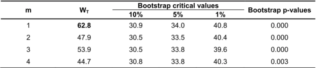
In the first step of the analysis, the null hypothesis of linearity against the alternative of threshold effects are tested for ER series. For this purpose, the Wald test WT

sta-tistics are calculated as reported in the previous section using Gauss program codes provided on Bruce Hansen’s Web page (www.ssc.wisc.edu/~bhansen/progs/ progs_threshold.html). The results of the Wald test, the bootstrap critical values gen-erated under the conventional significance levels, and the bootstrap p-values for threshold variables such that Zt ERt ERt m for delay parameters m from 1 to 4 can be seen in Table 1.

Table 1 The Results of Wald Test for Threshold Effects

m WT

Bootstrap critical values

Bootstrap p-values 10% 5% 1%

1 62.8 30.9 34.0 40.8 0.000

2 47.9 30.5 33.5 40.4 0.000

3 53.9 30.5 33.8 39.6 0.000

4 44.7 30.8 33.8 40.3 0.003

Note: *p-values are calculated from 10,000 replications.

(6)

It is seen from the table that all the statistics are significant at the 1% signific-ance level and support the existence of threshold effect or nonlinearity. Caner and Hansen (2001) propose selecting m that minimizes the residual variance. This is equivalent to selecting m that maximizes the value of the WT. As can be seen from

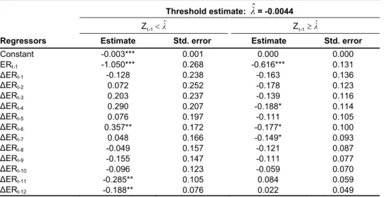
the table, the W_T statistic is maximized (W_T = 62.8) when m = 1. When the boot-strap p-values are recalculated for m = 1, we find it as 0.000 again. Following this result, which gives a strong support to the existence of a threshold effect in the US dollar/euro exchange rate, we estimate two-regime TAR model for m = 1 using least squares estimation method. The estimation results are given in Table 2.

Table 2 The Estimation Results of TAR Model

Threshold estimate: λˆ= -0.0044

ˆ

λ



t -1

Z Z_{t -1}λˆ

Regressors Estimate Std. error Estimate Std. error

Constant -0.003*** 0.001 0.000 0.000

ERt-1 -1.050*** 0.268 -0.616*** 0.131

ΔERt-1 -0.128 0.238 -0.163 0.136

ΔERt-2 0.072 0.252 -0.178 0.123

ΔERt-3 0.203 0.237 -0.139 0.116

ΔERt-4 0.290 0.207 -0.188* 0.114

ΔERt-5 0.076 0.197 -0.111 0.105

ΔERt-6 0.357** 0.172 -0.177* 0.100

ΔERt-7 0.048 0.166 -0.149* 0.093

ΔERt-8 -0.049 0.157 -0.121 0.087

ΔERt-9 -0.155 0.147 -0.111 0.077

ΔERt-10 -0.096 0.123 -0.059 0.070

ΔERt-11 -0.285** 0.105 0.084 0.059

ΔERt-12 -0.188** 0.076 0.022 0.049

Note: ***,** and * indicate statistically significance at the 1%, 5% and 10% significance levels, respectively.

Source: Author’s estimations.

The point estimate of threshold ( ˆλ) is found as -0.0044. This result indicates that TAR model splits the regression into two regimes, depending on whether the variable Z_t_₁ER_t_₁ER_t_₂ lies above or below -0.0044. The illustration of the two regimes can be seen in Figure 1.

The first regime is the case of Zt1-0.0044, which occurs when the deviation

of the ER falls, remains constant, or rises by less than -0.0044. The second regime is the case of Z_t₁-0.0044, which occurs when the deviation of the ER rises by more

(7)

Source: The author.

Figure 1 The ER Data, Classified by Threshold Regime

2.2 Robinson (1994) Test Results

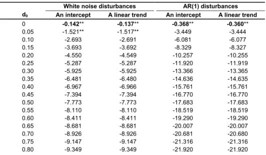
Following the paper of Caporale and Gil-Alana (2007), which extends the Robinson (1994) procedure to the case of nonlinear regression models, we apply the Robinson (1994) test procedure in the case of nonlinearity and estimate a two-regime TAR model instead of Eq. (1) as reported before. Then, we calculate the one-sided test statistics rˆ_{for the residuals obtained from the TAR model with}

0 0, 0.05, 0.10, 0.15, 0.20, 0.25,..., 0.50,...,1

d  . Under the null hypothesis H₀:dd₀,

the (0)I disturbances are modeled in both white noise and AR(1) processes for the case with a constant and the case with a linear trend. The results are reported in Table 3.

Table 3 Robinson Test Results for the Residuals from TAR Model

White noise disturbances AR(1) disturbances

d0 An intercept A linear trend An intercept A linear trend

0 -0.142** -0.137** -0.368** -0.360**

0.05 -1.521** -1.517** -3.449 -3.444

0.10 -2.693 -2.691 -6.081 -6.077

0.15 -3.693 -3.692 -8.329 -8.327

0.20 -4.550 -4.549 -10.257 -10.255

0.25 -5.287 -5.287 -11.920 -11.919

0.30 -5.925 -5.925 -13.366 -13.365

0.35 -6.481 -6.480 -14.636 -14.635

0.40 -6.967 -6.966 -15.761 -15.761

0.45 -7.394 -7.394 -16.770 -16.770

0.50 -7.773 -7.773 -17.683 -17.683

0.55 -8.110 -8.110 -18.519 -18.519

0.60 -8.411 -8.411 -19.290 -19.290

0.65 -8.681 -8.681 -20.007 -20.007

0.70 -8.926 -8.926 -20.681 -20.680

0.75 -9.147 -9.147 -21.316 -21.316

(8)

0.85 -9.533 -9.533 -22.497 -22.497

0.90 -9.702 -9.702 -23.051 -23.051

0.95 -9.858 -9.858 -23.584 -23.584

1.00 -10.002 -10.002 -24.100 -24.100

Note: The smallest value across the different values of d0. ** indicates nonrejection values of the null hypothesis at the 95%

significance level.

Source: Author’s estimations.

In the table, for a given d₀, significantly negative values of ˆr are consistent with the orders of integration smaller than d₀. A notable feature is the fact that ˆr

monotonically decreases with d₀. This is something to be expected because it is a one-sided test statistic. The results show that H₀ hypothesis cannot be rejected for

0

d = 0 and 0.05 in both cases with a constant and a linear trend if the disturbances are white noise. On the other hand, if the disturbances are assumed to be an AR(1) process, H₀ cannot be rejected for d₀ = 0 in cases with a constant and with a linear trend. It is clear that the lowest statistic across the different values of d₀ occurs when

0 0

d  in both disturbances. These findings show that the US dollar/euro exchange rate follows a stationary process, and there is a weak evidence of long memory only for white noise disturbances.

3. Conclusions

Following the paper of Caporale and Gil-Alana (2007), which examines both frac-tional integration and nonlinearities simultaneously in the same framework based on Robinson (1994) tests, this paper investigates the nonlinear behavior of the US dol-lar/euro exchange rate from January 1999 to August 2010 instead of assuming linear-ity and also allows for the possibillinear-ity of fractional values instead of using integer orders of integration. As a difference, we use a two-regime TAR model approach of Caner and Hansen (2001) for nonlinearity and different versions of Robinson (1994) tests for fractional integration. In the first step, the nonlinearity of the series is tested using Wald test as suggested by Caner and Hansen (2001), and a two-regime TAR model that allows to derive endogenous threshold effects is estimated. The results of the TAR model show that the point estimate of threshold is -0.0044, and around 23% of observation fall into the first regime, which is the case of Z_t₁-0.0044, whereas

around 77% of observations fall into the second regime, which is the case of Z_t_₁ -0.0044. In the second step of the analysis, we apply different versions of Robinson tests to the residuals obtained from the TAR model. Under the null hypothesis

0: 0

(9)

References

Baillie, Richard T., and Rehim Kilic. 2005. “Do Asymmetric and Nonlinear Adjustments Explain the Forward Premium Anomaly?” University of London, School of Economics and Finance Working Paper 543.

Ballie, Richard T., and George Kapetanios. 2005. “Testing for Neglected Nonlinearity in Long Memory Models.” University of London, School of Economics and Finance Working Paper 528.

Barkoulas, John T., and Christopher F. Baum. 1997. “Long Memory and Forecasting in Euroyen Deposit Rates.” Asia-Pasific Financial Markets, 4: 189-201.

Bond, Derek, Michael J. Harrison, and Edward J. O’Brien. 2007. “Modelling Ireland’s Exchange Rates: From EMS to EMU.” European Central Bank Working Paper 823. Bond, Derek, Michael J. Harrison, and Edward J. O’Brien. 2009. “Exploring Long

Memory and Nonlinearity in Irish Real Exchange Rates Using Tests Based on Semiparametric Estimation.” University College Dublin Centre for Economic Research Working Paper 01.

Caner, Mehmet, and Bruce E. Hansen. 2001. “Threshold Autoregression with a Unit Root.” Econometrica, 69(6): 1555–1596.

Caporale, Guglielmo M., and Luis A. Gil-Alana. 2007. “Nonlinearities and Fractional Integration in the US Unemployment Rate.” Oxford Bulletin of Economics and Statistics, 69(4): 521-544.

Diebold, Francis X., and Atsushi Inoue. 2001. “Long Memory and Regime Switching.” Journal of Econometrics, 105(1): 131-159.

Engel, Charles, and James D. Hamilton. 1990. “Long Swings in the Dollar: Are They in the Data and Forward Premium Anomaly?” American Economic Review, 80(4): 689-713. Gil-Alana, Luis A. 1999. “Testing of Fractional Integration with Monthly Data.” Economic

Modeling, 16(4): 613-629.

Gil-Alana, Luis A. 2000. “Mean Reversion in the Real Exchange Rates.” Economics Letters, 69(3): 285-288.

Gil-Alana, Luis A. 2001. “Testing of Stochastic Cycles in Macroeconomic Time Series.” Journal of Time Series Analysis, 22(4): 411-430.

Gil-Alana, Luis A. 2002. “Structural Breaks and Fractional Integration in the US Output and Unemployment Rate.” Economics Letters, 77(1): 79-84.

Gil-Alana, Luis A., and Peter M. Robinson. 1997. “Testing of Unit Roots and Other Nonstationary Hypothesis in Macroeconomic Time Series.” Journal of Econometrics, 80(2): 241-268.

Gil-Alana, Luis A., and Peter M. Robinson. 2001. “Testing of Seasonal Fractional Integration in the UK and Japanese Consumption and Income.” Journal of Applied Econometrics, 16(2): 95-114.

Granger, Clive W. J., and Roselyne Joyeux. 1980. “An Introduction to Long-Memory Time Series Models and Fractional Differencing.” Journal of Time Series Analysis, 1: 15-29. Hamilton, James D. 2001. “A Parametric Approach to Flexible Nonlinear Inference.”

Econometrica, 69(3): 537–573.

(10)

Kapetanios, George, and Yongcheol Shin. 2003. “Testing for Nonstationary Long Memory against Nonlinear Ergodic Models.” University of London, School of Economics and Finance Working Paper 500.

Mandelbrot, Benoit B. 1977. Fractals: Form, Chance, and Dimension. New York: Free Press.

Robinson, Peter M. 1994. “Efficient Tests of Nonstationary Hypothesis.” Journal of the American Statistical Association, 89: 1420-1437.

Sarno, Lucio, Giorgio Valente, and Leon L. Hyginus. 2004. “The Forward Bias Puzzle and Nonlinearity in Deviations from Uncovered Interest Parity: New Perspectives.” European Finance Association 2005 Moscow Meetings Paper.

Tong, Howell. 1978. “On a Threshold Model.” In Pattern Recognition and Signal Processing, ed. Chi Hau Chen, 575-586. Amsterdam: Sijhoff & Noordhoff.