Nuno Manuel Ortega Amaro
Mestre em Engenharia Electrotécnica e de Computadores
Study of AC losses in medium-sized
high temperature superconducting coils
Dissertação para obtenção do Grau de Doutor em Engenharia Electrotécnica e de Computadores
Orientador: João Miguel Murta Pina, Professor Doutor,
Universidade Nova de Lisboa
Co-orientadores: João Francisco Alves Martins, Professor Doutor,
Universidade Nova de Lisboa
José Maria Ceballos Martinez, Professor Doutor,
Universidad de Extremadura
Júri:
Presidente: Prof. Doutor Paulo da Costa Luís da Fonseca Pinto Arguentes: Prof. Doutor Mário Fernando da Silva Ventim Neves
Prof. Doutor Xavier Granados Garcia
Vogais: Prof. Doutor Alfredo Álvarez Garcia Prof. Doutor Paulo José da Costa Branco
Prof. Doutor João Miguel Murta Pina
iii
Study of AC losses in medium-sized High Temperature Superconducting Coils
Copyright © Nuno Manuel Ortega Amaro, Faculdade de Ciências e Tecnologia, Universidade Nova de Lisboa.
v
vii Looking back, I have to thank to so many people that it is almost impossible to write it down in a few lines. First of all I would like to thank to my three supervisors: Prof. João Murta Pina, Prof. João Martins and Prof. José Ceballos. Although the necessary hierarchical structure defines one supervisor and two co-supervisors I feel that this was really a team work and the experience and knowledge I gain from the three is similar. Thank you for all the moments, professional and personal, we had together.
To Doctors Fedor Gomory, Enric Pardo, Jan Souc and the remaining personnel from the Slovak Academy of Sciences, thank you for everything during my visit of three months to your laboratory. It was truly an honour to have the opportunity to work with you and to share some goods moments during my stay there.
I also would like to express my gratitude to the remaining professors in our section, from Faculdade de Ciências e Tecnologia da Universidade Nova de Lisboa. Prof. Mário Ventim, Prof. Anabela Pronto, Prof. Pedro Pereira and Prof. Stanimir Valtchev, and the remaining organization of the Electrical Engineering department. Thank you all not only for the help during the PhD work but also in the undergraduate and Masters Studies. It was that path that brought me here, today. A very warm and special thanks also for the remaining Professors of the Benito Mahedero – Group of Electrical applications of Superconductors from Universidad de Extremadura, Spain, for all the help given and kindness demonstrated during our many visits to Badajoz.
I also acknowledge the financial support given by Fundação para a Ciência e Tecnologia, through a PhD Scholarship with the reference SFRH/BD/78418/2011.
To my friends, Fábio Januário, Pedro Arsénio and Nuno Vilhena, thank you for walking alongside me during this long journey and for everything, in the good and not so good moments. Your time will come soon guys! To remaining colleagues, whose names are too many to state but the non-inclusion of a name does not necessarily means a forgetfulness of all help during these last four years.
Finally, I need to thank to all my family for supporting my choices and always being there when I needed.
Ana Rita, you cannot be included in this list. My thanks to you could not be expressed in words even if I had a true writing gift. To you I owe what I am today, and no matter what I will become you will always be there.
ix
Abstract
The study of AC losses in superconducting pancake coils is of utmost importance for the development of superconducting devices. Due to different technical difficulties this study is usually performed considering one of two approaches: considering superconducting coils of few turns and studying AC losses in a large frequency range vs. superconducting coils with a large number of turns but measuring AC losses only in low frequencies. In this work, a study of AC losses in 128 turn superconducting coils is performed, considering frequencies ranging from 50 Hz till 1152 Hz and currents ranging from zero till the critical current of the coils. Moreover, the study of AC losses considering two different simultaneous harmonic components is also performed and results are compared to the behaviour presented by the coils when operating in a single frequency regime.
Different electrical methods are used to verify the total amount of AC losses in the coil and a simple calorimetric method is presented, in order to measure AC losses in a multi-harmonic context. Different analytical and numerical methods are implemented and/or used, to design the superconducting coils and to compute the total amount of AC losses in the superconducting system and a comparison is performed to verify the advantages and drawbacks of each method.
xi
Resumo
O estudo de perdas AC em bobinas supercondutoras é de elevada importância para o desenvolvimento de dispositivos associados a esta tecnologia. Devido a diversas dificuldades de foro técnico os estudos presentes na literatura enquadram-se em uma de duas diferentes aproximações: estudo de perdas AC em bobinas com reduzido número de espiras mas considerando um espectro de frequências elevado ou estudo realizado em bobinas com um maior número de espiras, mas realizados apenas a frequências baixas, nomeadamente as frequências industriais de 50 ou 60 Hz. Neste trabalho, um estudo de perdas AC em bobinas de tamanho médio com um total de 128 espiras foi realizado, considerando um espectro de frequências desde 50 Hz até 1152 Hz e considerando correntes desde zero até à corrente crítica da bobina supercondutora. Adicionalmente, um outro estudo considerando mais do que uma harmónica de corrente a fluir em simultâneo na bobina também foi realizado, para verificar o efeito que este comportamento multi-harmónica poderá ter no valor total de perdas AC apresentado pela bobina.
Diferentes métodos de carácter eléctrico foram considerados para a medição das perdas AC nas bobinas supercondutoras e um método calorimétrico foi implementado para a determinação de perdas no contexto multi-harmónicas. Diferentes modelos analíticos e numéricos foram implementados e/ou utilizados, tanto para verificar as características das bobinas supercondutoras como para calcular a totalidade de perdas AC apresentadas pelas mesmas. Finalmente, foi efectuada uma comparação entre os diversos métodos e modelos utilizados, a fim de extrair as vantagens e desvantagens de cada um, no estudo de perdas AC em bobinas supercondutoras.
xiii
List of Contents
1. Introduction ... 1
1.1 Background and Motivation ... 1
1.2 Research Question & General Approach ... 2
1.3 Contents of this document ... 3
2. Theoretical Background ... 5
2.1. Superconductivity as a state of Matter ... 5
2.1.1. Historical Perspective ... 5
2.1.2. Macroscopic properties of Superconductors ... 6
2.1.3. Types of Superconductors ... 8
2.1.4. High Temperature Superconductivity ... 9
2.1.4.1 Historical perspective ... 9
2.1.4.2 Materials ... 10
2.1.5. Modelling of high temperature superconductors ... 15
2.1.5.1. Critical State Models ... 15
2.1.5.2. E-J Power Law ... 17
2.1.5.3. Numerical Modelling ... 18
2.2. Superconducting devices for power systems applications ... 21
2.3. AC Losses ... 23
2.3.1. Classification of losses in superconductors ... 23
2.2.1.1. Magnetization losses ... 23
2.2.1.2. Transport current losses ... 25
2.3.2. Models of AC losses ... 26
2.3.2.1. Analytical models ... 26
2.3.2.2. Numerical Models ... 27
2.3.3. AC Losses – from tapes to stacks and coils ... 28
2.3.4. Methods of measuring AC losses ... 29
2.3.4.1. Calorimetric ... 29
2.3.4.2. Electromagnetic ... 30
2.3.4.3. Comparison of AC losses measuring methods ... 31
2.3.5. Strategies for minimization of AC losses ... 32
2.3.5.1 Utilization of flux diverters ... 32
2.3.5.2 Roebel transposition ... 32
2.3.5.3 AC loss minimization in the manufacturing process ... 33
2.3.5.4 Other possible approaches for AC loss minimization ... 33
3. Modelling High Temperature Superconductors ... 35
3.1. Analytical models ... 35
3.2. Numerical models ... 42
xiv
3.2.2. FLUX2D Simulations ... 43
3.3. Concluding remarks ... 46
4. Experimental Setups ... 47
4.1. Critical current measurements ... 47
4.1.1. Superconducting tape ... 47
4.1.1.1. Self-field ... 48
4.1.1.2. Applied external field ... 48
4.1.2. Superconducting coils ... 49
4.2. AC losses measurement system ... 49
4.2.1. Electromagnetic method ... 49
4.2.2. Calorimetric method ... 52
4.3. Concluding remarks ... 55
5. HTS Coils Prototypes ... 57
5.1. Coil Implementation... 57
5.2. Critical Current Measurement ... 60
5.2.1. Critical current improvement by ferromagnetic shielding ... 63
5.2.2. Tape ageing and critical current degradation... 64
5.3. Concluding remarks ... 65
6. Measurement of AC losses ... 67
6.1. BSCCO tape samples ... 67
6.1.1. AC losses quantification ... 67
6.1.2. Frequency dependency ... 68
6.1.3. Comparison between models and experimental results ... 69
6.2. BSCCO coils ... 70
6.2.1. Magnetization losses ... 71
6.2.2. Transport current losses ... 72
6.2.2.1. Single frequency behaviour ... 72
6.2.2.2. Multi-harmonic behaviour ... 79
6.2.2.3. Frequency dependence analysis ... 83
6.2.3. Comparison between models and experiments ... 85
6.3. Concluding remarks ... 89
7. Conclusions and Future Work ... 91
Original contributions ... 93
xv
List of Figures
Figure 2.1. Superconductivity concise timeline ... 5
Figure 2.2. Experiments made by Onnes using Mercury. Abscissa is resistance (as a fraction of resistance value at 0 °C) and ordinate is temperature in Kelvin. Source: (Onnes 1913). ... 6
Figure 2.3. T - J - H phase diagram ... 7
Figure 2.4. Known elements with superconductivity properties. Source: www.superconductors.org ... 8
Figure 2.5. Type I superconductor ... 9
Figure 2.6. Type II superconductor ... 9
Figure 2.7. PIT process. Source: (Ceballos 2010). ... 11
Figure 2.8. Bi-2223 superconducting tape produced by Bruker HTS GmbH (http://bruker-est.com/). ... 12
Figure 2.9. Degradation of critical current value with the increase of magnetic field in a Bi-2223 tape manufactured by American Superconductor (AMSC) (http://www.amsc.com/)... 12
Figure 2.10. Performance of 1G and 2G tapes under applied magnetic field. Source: http://www.theva.com ... 13
Figure 2.11. RABiTS™ technique (adapted from (Hammerl et al. 2002)). ... 13
Figure 2.12. 2G HTS Tape manufactured by Super Power (source: http://www.superpower-inc.com/) ... 15
Figure 2.13. 2G HTS Tape manufactured by AMSC (source: http://www.amsc.com/) ... 15
Figure 2.14. Superconducting slab with infinite dimensions in y and z and 2a width in x. ... 16
Figure 2.15. B-H relation in a superconductor. ... 16
Figure 2.16. Current Density and magnetic field distribution in a superconducting slab considering Bean Model. ... 17
Figure 2.17. E-J Power Law for different values of n parameter. ... 18
Figure 2.18. Cross section (x-y plane) of an infinite superconductor in z direction. ... 18
Figure 2.19. Shielding and coupling currents in a 1G HTS tape. Adapted from (Ceballos 2010). 24 Figure 2.20. Lock-in Amplifier method for measurement of AC losses configuration. ... 30
Figure 2.21. Roebel transposition consisting on sixteen 2G HTS tapes. Source: (Goldacker et al. 2007). ... 33
Figure 3.1. Dimensions of a pancake coil: mean radius (a), height (b), and total width (c). ... 36
Figure 3.2. Dimensions of a set of two concentric coils. ... 38
Figure 3.3. Computation of the inductance of an HTS coil. ... 39
Figure 3.4. Computation of inductance in function of internal radius of a coil. ... 40
Figure 3.5. Computation of the total mutual inductance of an HTS coil, composed of several single pancake coils. ... 41
Figure 3.6. Critical current dependence of applied magnetic field for the used 1G HTS tape. .. 43
Figure 3.7. FLUX2D model of a cross section of 1G HTS tape. ... 44
Figure 3.8. Geometry of an HTS coil with 8 turns. ... 44
Figure 3.9. Equivalent electric circuit for a coil with 8 turns. ... 45
xvi
Figure 4.1. HTS sample for critical current measurement. ... 48
Figure 4.2. LIA Method for AC loss measurement. ... 49
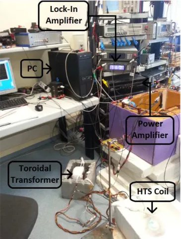
Figure 4.3. AC losses measurement system used at the Slovak Academy of Sciences. ... 50
Figure 4.4. Detail of copper wire position in a 4 cm contactless loop: real tape (left) and schematic (right). ... 51
Figure 4.5. Position of AC losses measuring methods in the HTS coil. ... 52
Figure 4.6. Cylindrical capacitor. ... 52
Figure 4.7. Cylindrical capacitor with two different dielectrics. ... 53
Figure 4.8. Implemented cylindrical capacitor. ... 54
Figure 5.1. Sample of HTS tape for critical current measurement (adapted from (Arsénio 2012)). ... 58
Figure 5.2. Curve fitting for critical current determination. ... 58
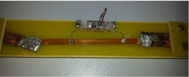
Figure 5.3. Implemented HTS coils. ... 59
Figure 5.4. Experimental setup for measurement of critical current in an HTS coil. ... 60
Figure 5.5. Critical current measurements in the two implemented HTS coils. ... 61
Figure 5.6. Critical current of a set of two HTS coils with and without connection losses. ... 62
Figure 5.7. Comparison of simulated and experimentally obtained critical current of an HTS coil with 128 turns. ... 62
Figure 5.8. Critical current improvement by adding flux diverters. ... 63
Figure 5.9. Thermal cycles effect on critical current. ... 64
Figure 6.1. AC losses in a sample of HTS tape (experimental results). ... 68
Figure 6.2. Microphotography of the used HTS tape. ... 69
Figure 6.3. AC losses in a sample of HTS tape without the eddy currents component. ... 69
Figure 6.4. Comparison between experimental results and Norris ellipse model. ... 70
Figure 6.5. Magnetization losses under applied magnetic field. ... 71
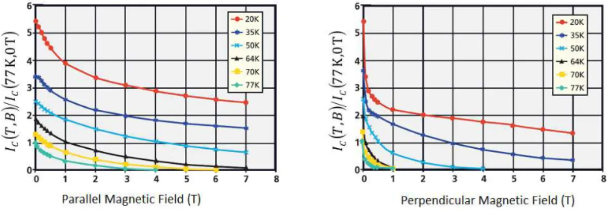
Figure 6.6. Measurements of AC losses in two implemented coils. ... 73
Figure 6.7. Comparison between experimental and phase corrected data. ... 74
Figure 6.8. Measured AC losses at 144 Hz using three different methods. ... 75
Figure 6.9. AC losses measuring methods comparison for 72, 144 and 288 Hz. ... 75
Figure 6.10. AC losses measurements for frequencies between 72 Hz and 1152 Hz. ... 76
Figure 6.11. Measured AC losses for frequencies between 288 Hz and 576 Hz. ... 77
Figure 6.12. Measured AC losses for frequencies between 576 Hz and 1152 Hz. ... 77
Figure 6.13. Comparison of measured AC losses using a 4 cm voltage taps and a contactless loop configurations. ... 78
Figure 6.14. Measured AC losses in a 32 turn coil at 288 Hz. ... 78
Figure 6.15. Measured AC losses at 288 Hz considering two contactless loops. ... 79
Figure 6.16. Multi-harmonic generation system. ... 80
Figure 6.17. Measured AC losses for 50 Hz and its 5th and 7th harmonic. ... 80
Figure 6.18. Eddy currents component subtraction in measured AC losses in HTS coils. ... 84
Figure 6.19. Frequency dependence behaviour of AC losses. ... 85
Figure 6.20. Comparison of AC losses obtained experimentally and by an analytical model. ... 86
Figure 6.21. MEMEP simulations: different n-values comparison. ... 87
Figure 6.22. MEMEP simulations: different cross-sections comparison. ... 87
Figure 6.23. AC losses at 144 Hz: simulation results VS experimental data. ... 88
xvii
List of Tables
Table 2.1. High temperature superconductors ... 10
Table 3.1. Geometric parameters used in the MEMEP simulations. ... 42
Table 3.2. Geometric parameters for FLUX2D simulations of HTS coils. ... 45
Table 3.3. Characteristics of materials used in simulations. ... 45
Table 5.1. HTS tape characteristics. ... 57
Table 5.2. Results of analytical method for coil design. ... 59
Table 5.3. Inductance of a set of two coils. ... 60
Table 5.4. Results of cftool for determination of coils characteristics. ... 61
xix
Symbology
B Magnetic flux density (T).
Bi Experimentally verified constant used in Kim Model.
C Capacitance (F).
C1 CylindricalCapacitor 1. C2 CylindricalCapacitor 2.
C1LN2 Capacitance of cylindrical capacitor 1 when fully immersed in liquid nitrogen (pF) C2LN2 Capacitance of cylindrical capacitor 2 when fully immersed in liquid nitrogen (pF) d thickness of superconducting tape or superconducting layer (mm).
D Internal diameter of a superconducting coil (mm). ∆Hvap Latent heat of vaporization of nitrogen (198.99 kJ/kg).
E Energy (J).
E Electric Field (V/m).
EC Critical Electric Field (1 µV/cm).
ESC Electric field inside a superconductor.
esp Thickness of a superconducting tape.
f Frequency (Hz).
g distance between two adjacent superconducting coils (mm).
H Magnetic Field (A/m).
H Height of nitrogen in a cryostat (m).
h distance between superconducting regions of two adjacent superconducting tapes (mm).
HC Critical Magnetic Field (A/m).
I DC current applied to a superconducting tape or coil (A). Ip (or Im) Amplitude of an AC current flowing in a superconductor (A). J Current Density (A/m2).
xx JC0 Critical Current Density achieved in self-field conditions (A/m2).
JSC Critical Current Density inside a supercondutor (A/m2).
L Self-inductance (H).
l Perimeter of outer filament in a superconducting tape (mm) or length of superconducting tape used in a coil (m).
LC Loss Power per cycle per unit of length (W/m).
LM Mutual Inductance (H).
m Mass (kg).
n coefficient of the power law in a superconductor. N number of turns in a coil.
Ped Loss power due to eddy currents per cycle per unit of length (W/m). Pr Resistive loss power per cycle per unit of length (W/m).
Q Energy loss per cycle per unit length (J/m). R Electrical resistance (Ω).
Rconnection Resistance of an electric connection between two superconducting coils (Ω). r1 Internal radius of a cylindrical capacitor (mm).
r2 External radius of a cylindrical capacitor (mm). Ri Internal radius of a superconducting coil (mm). Re External radius of a superconducting coil (mm). S Section of superconductor (mm2).
SC Section of a cryostat (mm2).
T Working Temperature (K).
TC Critical Temperature (K).
U Voltage (V).
w width of a superconduting tape (mm).
ε Permittivity of medium (F/m).
ε0 Permittivity of vacuum (8.854 x 10⁻¹² F/m). µ0 Vacuum permeability (4 x π x 10-7 H/m).
ρ Resistivity (Ω.m).
xxi
Acronyms
1G Superconducting tape of first generation, in Bi-2212 or Bi-2223. 2G Second generation superconducting tape manufactured from YBCO.
AC Alternating current.
AMSC American Superconductor.
BaLaCuo First high temperature superconductor discovered. BLCO same as BaLaCuO.
Bi-2201 High temperature superconductor with a chemical composition of Bi2Sr2Ca0Cu1O6.
Bi-2212 High temperature superconductor with a chemical composition of Bi2Sr2Ca1Cu2O8.
Bi-2223 High temperature superconductor with a chemical composition of Bi2Sr2Ca2Cu3O12.
BSCCO One of the three forms of the superconductor above. BiSrCaCuO same as BSCCO.
DC Direct Current, in opposition to alternative current. FEA Finite Element Analysis.
FEM Finite Element Method or Finite Element Modelling.
HBCCO High temperature superconductor with a chemical composition of HgBa2Ca2Cu3O1+x.
HgBaCaCuO same as HBCCO.
HTBCCO High temperature superconductor with a chemical composition of Hg0.8Tl0.2Ba2Ca2Cu3O8+δ.
HgTlBaCaCuO same as HTBCCO.
HTS High Temperature Superconductivity / Superconductor. IBAD Ion Beam Assisted Deposition.
LIA Lock-In Amplifier.
xxii PDE Partial Differential Equation.
PIT Powder In Tube.
RABiTS Rolling-Assisted Biaxially Textured Substrate. SFCL Superconducting Fault Current Limiter.
SFCLT Superconducting Fault Current Limiting Transformer. SMES Superconducting Magnetic Energy Storage.
TFA-MOD Trifluoroacetate Metal Organic Deposition.
XPS Extruded polystyrene.
Y-123 Superconducting phase of YBCO.
YBaCuO High temperature superconductor with a chemical constitution of YBa2Cu3O7-δ.
1
1.
Introduction
1.1
Background and Motivation
Electric grids are operating in a particular challenging context in the last years. The necessity for a high quality power and different environmental protection laws are forcing grid operators to surpass different technological challenges and to change completely the concept of electric grid. With this change arises the opportunity for new devices and new technologies, having always as goals the improvement of power quality while reaching a sustainable energy system. One such technology, whose applications are envisaged to promote this change in electric grids, is superconductivity.
Different superconducting devices can be applied in power grids and their unique characteristics make them valid candidates to solve different problems in the existing grids. Through the whole world, different research groups focus their interest in these devices and their applications to power systems (Tixador 2010; Fujiwara et al. 2010; Xiao et al. 2012). However, superconductors still have different technological problems that need to be solved, in order to reach a maturity state to apply in a large scale context. One of such challenges, which concentrate a huge investigation effort, is the existence of AC losses. When operating in DC conditions, superconductors present a virtual zero resistance, a unique and very important characteristic which by itself could solve different problems in power grids such as transport losses. However, when operating in AC conditions a component of AC losses is generated. Considering that superconductors operate at cryogenic temperatures, it is necessary to extract all heat generated in the system and the existence of AC losses results in a higher amount of heat loss, which evidently results in the need to have higher power cryogenic systems, when comparing with DC operation. Therefore, the study of AC losses, which includes the mechanisms that originate them, creation and development of methods to measure them and minimization strategies, is a key to improve the performance of superconducting devices and their applicability. In addition to this, superconducting materials are still costly, which results in high implementation costs for any project. Considering this, the creation of accurate models is a very important step, in order to allow the simulation of superconducting devices and extract their behavioural characteristics to apply to real systems. Different models, with different levels of complexity can be used, not only to calculate AC losses but so simulate the overall system.
One of the superconducting elements that is most vastly used in devices is the superconducting pancake coil. Therefore, the study of AC losses in pancake coils is of utmost importance. Although this study has been already performed for years, there is still space for innovation in this area. The coil inductance allied to the high currents that can flow through the superconductor will result in high voltages at the coil ends, making the process of measuring AC losses a complex one. The need for accurate models is even more important considering this aspect.
2 Taking into account the different considerations present in the last few paragraphs, this work aims to contribute to the study of AC losses in medium-sized (more than one hundred turns) superconducting coils, through the implementation of measuring processes and validation of different models. The study of AC losses is usually performed considering two different conditions: small coils considering a large frequency spectrum or larger coils, but considering only the industrial frequency (50 Hz or 60 Hz). In this work, a study of AC losses in medium sized coils will be performed for a frequency range of 50 Hz to 1152 Hz considering different measuring methods and different models.
1.2
Research Question and General Approach
As mentioned before, the application of superconducting devices in power systems in order to increase power quality is desirable. Many of these devices use a common superconducting element: superconducting pancake coils. Although they have unique characteristics, superconductors present AC losses when in present of an AC magnetic field, or when flown by an AC current. Since these losses will generate heat that must be extracted from the cryogenic system in which the superconducting device is immersed, the study of AC losses in superconducting pancake coils is of upmost importance to the development of superconducting devices. Considering this, the main research question chosen to guide this work is the following:
Research Question (Q1)
What is the behavior demonstrated by AC losses in medium-sized superconducting coils when subjected to currents considering a high frequency range, in comparison to that demonstrated by smaller coils and samples of superconducting tape?
Proposed hypothesis to address this research question is:
Hypothesis
If measuring methods used to measure AC losses in other superconducting components can be applied to medium-sized coils at high frequencies, within safe operating conditions, then the behavior presented by these coils can be correctly evaluated and compared to that obtained by other superconducting elements, providing an advance in the study of AC losses in superconducting pancake coils.
In addition to this research question, some more specific research questions can be formulated:
Q1 a)
Are methods used to measure AC losses in samples of superconducting tape applicable to coils with a high number of turns and a high working frequency?
Q1 b)
Do existing models, both analytical and numerical, present good results when considering AC losses in superconducting coils with a high number of turns?
Q1 c)
Do AC losses have a linear behavior when more than one current harmonic is flowing in the superconducting coil, i.e., is the total amount of AC losses the sum of the losses components originated by the different frequency harmonics or is there a new component?
3
Consider the different existing methods to measure AC losses and apply them to medium-sized superconducting coils;
Compare results obtained with the different methods and if necessary try to adjust the existing methods to improve results, or consider the creation of new measuring methods;
Simulate the behavior of a test superconducting coil, in order to verify the applicability of numerical and analytical models.
1.3
Contents of this document
This thesis is organized in five different chapters, excluding the present one and one for conclusions, which aims not only to summarize results obtained but also to give some future work possibilities within this line of research and present the original contributions of this work to the scientific field in study. A brief description of the remaining chapters is now given, in order to give the reader an overall view of the document organization.
Chapter 2 – Theoretical Background: this section is made of a literature revision of superconducting devices systems and associated technologies. Since superconductivity is not a conventional field in the framework of Electrical Engineering, a brief historical perspective is presented. After that, the literature review is focused in AC losses, describing their origins, measuring methods and evolution when increasing the superconducting device complexity.
Chapter 3 – Modelling of High Temperature Superconductors: for a successful application of superconducting devices in power systems, a first phase of modelling is usually performed in order to achieve the desirable system characteristics. Different implemented models in this work are contained in this section of the document, together with other models that are used here but whose implementation was performed by other research groups along the years. All models described have as a goal the computation of AC losses, even if they can easily be used for other goals.
Chapter 4 – Experimental Setups: different experimental setups were implemented, with the objective of verifying the main characteristics of the different elements used in this thesis. The implementation process of every experimental setup is described in this section.
Chapter 5 – HTS Coils Prototypes: this section contains a description of the implementation process of different superconducting coils, which are the test elements in this work. Measurements performed in those coils, in order to verify their characteristics, are also presented in this chapter.
5
2.
Theoretical Background
2.1.
Superconductivity as a state of Matter
Superconductivity is a vast field of knowledge, with more than 100 years of associated research. Consequently it is not feasible to describe in a document such as a thesis all associated phenomena and characteristics of superconducting materials. However, it is also not logical to realize a work in this area without addressing the main phenomena related to it. Thus, a short description of superconductivity and basic characteristics of materials used in this work will be presented.
2.1.1.
Historical Perspective
Figure 2.1 shows a summarized timeline with the most significant discoveries related to superconductivity. Some of these discoveries, although very important to the general knowledge of this phenomenon, are out of the scope of this thesis, thus will not be addressed.
Figure 2.1. Superconductivity concise timeline
The term “superconductivity” was first used by Heike Onnes, in 1911. In his laboratory in the Netherlands, this scientist verified that the electrical resistance of capillaries of mercury abruptly disappeared at temperatures below 4.2 K. This was the discovery of a new state of matter, as Onnes stated at his Nobel Prize winning speech in 1913 (Onnes 1913):
“Thus the mercury at 4.2 K has entered a new state, which, owing to its particular electrical properties, can be called the state of superconductivity”
Figure 2.2 depicts the experiments made by Onnes, where an abrupt loss of resistivity in Mercury can be clearly seen at 4.2 K. The temperature below which a material becomes superconducting is called critical temperature.
6 Figure 2.2. Experiments made by Onnes using Mercury. Abscissa is resistance (as a fraction of resistance value at 0 °C) and ordinate is temperature in Kelvin. Source: (Onnes 1913).
In 1933, Walter Meissner and Robert Ochsenfeld discovered that superconductors exhibit perfect diamagnetism, i.e. they fully expel magnetic flux from their core (Meissner & Ochsenfeld 1933). This effect, henceforth known as Meissner Effect, fully separates superconductivity from perfect conductivity (in which a material has zero resistance, but is a perfect flux conservation medium, rather than a perfect diamagnet).
Two decades later, in 1957, Alexei Abrikosov foretold the existence of a new type of superconductors, to which he called type II superconductors, in opposition to the already known superconductors (then known as type I). These new superconductors allowed the existence of a mix state, in which the material would undergo a progressive penetration of the magnetic flux in its interior in flux quanta well defined (flux vortices). A superconducting state and a normal state would then co-exist in the material. Also in 1957, John Bardeen, Leon Cooper and John Schrieffer elaborated a theory known as BCS theory to explain the microscopic behaviour of superconductors. This is the more consensual theory in superconductivity and states that pairs of electrons (known as Cooper pairs) act as charge carriers in superconductors.
In 1986 two IBM researchers, Georg Bednorz and Alexander Müller, discovered High Temperature Superconductivity (HTS) in ceramic compounds (Bednorz & Müller 1986). This was a breakthrough because some of these compounds are superconductors at temperatures above 77 K (liquid nitrogen boiling temperature), thus allowing the utilization of nitrogen instead of helium as a cryogenic fluid. Due to their discoveries, these researchers were awarded the Nobel Prize in Physics in 1987. The discovery of HTS was the initial step to conceive technical and economically viable applications of superconductivity in power systems.
2.1.2.
Macroscopic properties of Superconductors
Superconductivity presents unique macroscopic properties. These properties include:
Zero resistivity
Below a temperature defined as critical temperature, TC, superconductors present virtually
7 Considering a superconducting ring with resistance R and inductanceL, imposing a current 0
I
in the ring, the evolution of current flowing in the ring is given by
t
e I t
i( ) 0 (2.1)
where
R
L
is the time constant of the ring. Being the ring in a superconducting state it canbe seen that
whileR
0
. This means thati
(
t
)
I
0,
t
0
, i.e. the current does not decay with time. Measurements indicate that resistivity in a superconductor in which flows a DC current is at the order of10
25 Ω∙m,17
orders of magnitude below copper (Orlando & Delin 1991).Meissner Effect
Meissner Effect is a fundamental characteristic to distinguish superconductivity from perfect conductivity. Discovered by Meissner and Ochsenfeld (Meissner & Ochsenfeld 1933) this effect verifies an expulsion of magnetic field from the interior of a superconductor. This expulsion is due to the appearance of shielding currents flowing in the surface of the superconductor which completely shield the superconducting core.
T – J – H phase diagram
In order not to lose superconductivity, i.e. in order not to achieve a phenomenon designated as quench, superconductors must stay between certain working limits. These limits include not only the already mentioned current density and temperature but also the magnetic field. These three quantities are not independent from each other. Instead, they relate in a phase diagram usually called T J H diagram. Figure 2.3 shows a typical surface of a T J H phase diagram.
Figure 2.3. T - J - H phase diagram
It is important to notice that in order to maintain superconductivity, a superconducting material must obey simultaneously the three following conditions:
T
T
C;
H
H
C;
J
J
C;
8
2.1.3.
Types of Superconductors
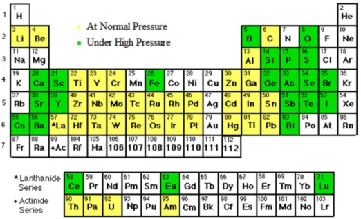
Since the discovery of Onnes in 1911, further investigations during the 20th century found that superconductivity is a thermodynamic phase that many elements can achieve. In fact, around half of known elements can act as superconductors. However, some of these elements require high pressures to achieve a superconducting state whilst others can achieve it at atmospheric pressure. Figure 2.4 shows a periodic table of elements where elements that can reach a superconducting state are highlighted and in which pressure conditions they can achieve such state.
Figure 2.4. Known elements with superconductivity properties. Source: www.superconductors.org Even if there are many elements that can reach a superconducting state, in real applications only a few are used. These are often compounds involving several elements, not pure elements. The discovery of superconductivity in the diverse known elements happened during several decades and were the foundation to discover microscopic and macroscopic properties of superconductivity. Nonetheless, all superconductors can be included in one of two types:
Type I Superconductors
9 Figure 2.5. Type I superconductor
Type II Superconductors
In 1957, Alexei Abrikosov theoretically predicted a different kind of superconductors from those already known (Abrikosov 1957). With this discovery, aroused the need for a separation of types of superconductors, which originated the designation of type I and type II. Abrikosov defended that a third state could exist in the material, besides Meissner and normal states. This was called mix state and it consisted in the coexistence of a superconducting and a normal state in the material. This means that some parts of the superconductor are penetrated by magnetic flux in well-defined flux quanta while others are not. The typical behaviour of type II superconductors is illustrated in Figure 2.6.
Figure 2.6. Type II superconductor
Type II superconductors are usually metal compounds and alloys with the exception of Niobium (French 1968), Technetium (Daunt & Cobble 1953) and Vanadium (Wexler & Corak 1952). These (type II) are the only superconductors with real applications. One very important kind of superconductors included in type II are the high temperature superconductors, described in next section.
2.1.4.
High Temperature Superconductivity
2.1.4.1 Historical perspective
10 were poor conductors at room temperature and offered a new perspective because till that time it was thought that superconductivity was associated to good electric conductors (at room temperature). In addition to this, it was thought that the critical temperature of superconductors would not increase much above 20 K (Burns 1992). One important thing to notice is that high temperature superconductors do not obey BCS theory and the current transport mechanism in this superconductors is still not clear (Burns 1992).
The discovery of BLCO led to a search for superconducting characteristics in ceramic materials, increasing critical temperatures in several dozens of degrees in the last 30 years. Table 2.1 contains a list of some high temperature superconductors discovered in the last three decades. Although this is not a consensual opinion for all authors, in this work it is considered high temperature superconductors as materials whose critical temperatures are above 77 K (boiling temperature of Nitrogen), with the exception of BLCO.
Table 2.1. High temperature superconductors
Material (acronym) Critical Temperature (K) Reference
BaxLa5-xCu5O5-(3-y) (BLCO) 30 (Bednorz & Müller 1986) Y1.2Ba0.8CuO4-δ (YBCO) 93 (Wu et al. 1987)
BiSrCaCu2Ox (BSCCO) 105 (Maeda et al. 1988) TlBa2Ca3Cu4O11 (TBCCO) 128 (Ihara et al. 1988) HgBa2Ca2Cu3O1+x (HBCCO) 133 (Schilling et al. 1993) Hg0.8Tl0.2Ba2Ca2Cu3O8+δ (HTBCCO) 138 (Dai et al. 1995)
HgBa2Ca2Cu3O8+δ (HBCCO)* 153 (Chu et al. 1993) * at a pressure of 150 kbar (148 katm).
2.1.4.2 Materials
From all discovered high temperature superconductors there are two compounds with greater importance, in terms of their applicability to industrial systems:
Bi2Sr2CanCun+1O6+2n (BSCCO) with n = 0, 1, 2.
YBa2Cu3O7-δ (YBCO).
BSCCO is usually present in two of three phases where it presents superconductivity. These two phases, Bi-2212 (n = 1) and Bi-2223 (n = 2), have critical temperatures of respectively 92 K and 110 K. Despite the fact that Bi-2223 has higher critical temperature (110 K comparing to 92 K) and higher critical current density than Bi-2212, this one has the advantage of having a lower degradation in its properties in the presence of magnetic fields, so both phases are produced and commercialized. Bi-2201 (n = 0) is also superconductor but its critical temperature is around 40 K thus cannot be cooled using liquid nitrogen.
11
Superconducting Tapes
Superconductors used in power systems applications are usually presented in two forms, either bulk or tape.
Since this work is based only in superconducting tapes, no further description of bulk materials is made. Nonetheless, the characteristics of materials here presented are valid for both tapes and bulk superconductors. The most common types of HTS tape available on the market are made using one of two materials:
BSCCO (Bi2Sr2CanCun+1O6+2n with n = 1, 2) – also called first generation (1G) tape.
YBCO (YBa2Cu3O7-δ) – used more recently than the BSCCO tape, forms the basis of the second generation (2G) tape.
A short description of production processes and characteristics of both 1G and 2G tapes are presented in this section, to verify the differences between these materials.
First Generation HTS Tapes
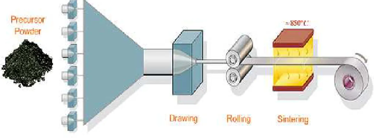
BSCCO tapes (or 1G tapes) are manufactured using a technique called Powder In Tube (PIT) (Grivel & Flükiger 1996). PIT process can be described very shortly as follows. Small silver tubes are filled with a precursor powder of superconducting material with one or more filaments (the number of superconducting filaments depends on the manufacturer). Obtained tubes are then brought together in a larger silver capsule which is then subjected to a process of drawing and rolling. The tape is then sintered at a temperature around 850 °C which allows a controlled growth of the superconductor with high degree of alignment between the grain boundaries, fundamental characteristic to achieve a high critical current density. PIT process is schematized inFigure 2.7. Even considering the additional robustness given by silver, 1G HTS tapes are still fragile due to the fact that the superconducting material is ceramic. These tapes have a maximum bending radius of a few dozen of millimetres which can limit their applications.
Figure 2.7. PIT process. Source: (Ceballos 2010).
12
a) Cross section of a Bi-2223 tape with 121 superconducting filaments (grey) embedded in a silver matrix (white).
b) Aspect of Bi-2223 superconducting tape
Figure 2.8. Bi-2223 superconducting tape produced by Bruker HTS GmbH (http://bruker-est.com/). One of the main issues of 1G superconducting tapes is the fast degradation of its critical current value with increasing applied magnetic field. This behaviour can be seen in Figure 2.9. Even considering temperatures around 20 K it is possible to see this fast degradation. Continuous research efforts regarding superconducting materials led to the creation of a new kind of superconducting tape – 2G HTS tape – with an improved behaviour under magnetic fields.
Figure 2.9. Degradation of critical current value with the increase of magnetic field in a Bi-2223 tape manufactured by American Superconductor (AMSC) (http://www.amsc.com/).
Second Generation HTS Tapes
13 Figure 2.10. Performance of 1G and 2G tapes under applied magnetic field. Source:
http://www.theva.com
These tapes are manufactured using YBCO (phase Y-123), and are commonly designated as coated conductors. The process has four main steps:
Preparation of the substrate;
Deposition of intermediate layers;
Deposition of superconducting layer (YBCO);
Addition of connection and stabilizing layers.
Step 1 – Preparation of the Substrate
There are two different techniques to do the preparation of substrate for 2G tapes. One is to use an alloy of nickel-tungsten subjected to a technique called Rolling-Assisted Biaxially Textured Substrate (RABiTS™). This method, schematized in Figure 2.11, is used by several manufacturers including American Superconductor (AMSC) (Rupich et al. 2007).
Figure 2.11. RABiTS™ technique (adapted from (Hammerl et al. 2002)).
14 Step 2 – Deposition of intermediate layers
After the preparation of substrate it is necessary to implant a series of layers prior to the deposition of the superconducting layer. These layers are called Epitaxial Buffer Layers. Main functions of buffer layers include:
Provide a surface for the epitaxial growth of the superconductor;
Protect the superconductor of possible contaminations from the substrate;
Facilitate the adhesion of the superconductor, avoiding a possible peeling effect.
Since there are two different methods for preparing the substrate, the deposition of intermediate layers is also different for each case. In the case where RABiTS™ was used to prepare the substrate, a sputtering technique is used for the deposition of the intermediate layers (Goyal et al. 2004). In the case of manufacturers that used an untextured substrate sputtering is insufficient to implant the intermediate layers. In this case, a technique called Ion Beam Assisted Deposition (IBAD) is used. This technique combines ion implantation with sputtering, allowing an adequate deposition of the different intermediate layers (Selvamanickam et al. 2001).
Step 3 – Deposition of superconducting layer
Deposition of YBCO layer is also implemented using different techniques depending on the manufacturer. AMSC uses a technique denominated as Trifluoroacetate Metal Organic Deposition (TFA-MOD) (McIntyre et al. 1995). This technique consists in a chemical deposition of the YBCO layer using a trifluoroacetate precursor and subsequent pyrolysis. In the case of SuperPower, a different method called Metal-Organic Chemical Vapour Deposition (MOCVD) is used (Selvamanickam et al. 2001). In this method, a chemical vapour is deposited in the substrate and pyrolysis is used to form the epitaxial layer of YBCO.
Step 4 Addition of connection and stabilizing layers
In order to protect the superconducting layer and to add mechanical stability to the HTS tape a series of connection and stabilizing layers are added. A silver layer is added to permit electrical connections and a coating (usually copper) is added to minimize tape deterioration due to mechanical stresses.
15
a) Layers diagram b) Actual aspect of the tape
Figure 2.12. 2G HTS Tape manufactured by Super Power (source: http://www.superpower-inc.com/)
a) Layers diagram b) Actual aspect of the tape
Figure 2.13. 2G HTS Tape manufactured by AMSC (source: http://www.amsc.com/)
2.1.5.
Modelling of high temperature superconductors
Accurate models are often needed when designing devices employing superconducting materials, in order to verify their behaviour. Even if a consensual theory is not yet formulated to explain the current transport mechanism in HTS, there are several models that describe the behaviour of these material with accurate results.
2.1.5.1. Critical State Models
Critical state models are the simplest option to describe the behaviour of high temperature superconductors. Based in macroscopic properties of the material, these models are obtained by experiments verifying the relation between current density and magnetic field in the superconductor. They assume that the local current density can only have three different values, namely
J
C,0
or
J
C whereJ
C is critical current density. When a superconductor is16
Bean Model
Bean Model considers that current density and flux density are independent (Bean 1964). This means that when a magnetic field is applied, the value of current density in the superconductor will always assume the critical value, as already stated. To simplify the model, Bean assumed that the superconductor slab has infinite dimensions in x and zdirections and width
2
a
iny
direction and is immersed in a magnetic field oriented in z direction, as shown in Figure 2.14.Figure 2.14. Superconducting slab with infinite dimensions in y and z and 2a width in x. Since dimension
2
a
is very thin compared to other dimensions of the slab, only the magnetic field component which is parallel to the slab cross section (xdirection component of the magnetic field) needs to be considered.Ampère Law is still valid in the interior of the superconductor and can be written as follows.
J B
0 (2.2)
This happens because macroscopically a superconducting material can be considered as non-magnetic, and it is assumed that there is a uniform penetration of flux density in the superconductor, in the operating zone, as shown in Figure 2.15.
Figure 2.15. B-H relation in a superconductor.
Since the only variation will happen in x direction, equation (2.2) can be rewritten as
x
x
e
e
(
)
)
(
0
J
y
dy
y
dB
x
(2.3)17 the increasing of the magnetic field the current density penetrates more in the superconductor till it reach full penetration. Figure 2.16 demonstrates this behaviour.
Figure 2.16. Current Density and magnetic field distribution in a superconducting slab considering Bean Model.
Other Critical State Models
In addition to Bean Model there are other more complex critical state models. One of these models also very used in engineering applications is the Kim Model (Kim et al. 1962; Kim et al. 1963). Unlike Bean Model, in this case the current density is not independent from the applied magnetic field. Instead, there is a relation between those entities given by:
i C C
B
B
J
B
J
1
)
(
0 (2.4)In this equation
J
C0 is the critical current density obtained at self-field;B
i is a constant obtained experimentally.Other critical state models like Exponential Model (Fietz et al. 1964), Power Model (Irie & Yamafuji 1967) or Linear Model (Watson 1968) can also be chosen, but are not used so often as the previous two.
2.1.5.2. E-J Power Law
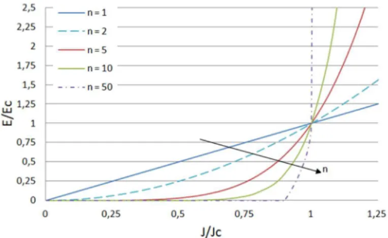
Critical state models are based on the assumption that currents in the superconductor always assume its critical value. However, in type II superconductors and especially in HTS, the current does not always present its critical value and the latter does not represent an abrupt transition between a superconducting state and a normal state. To achieve higher precision, it was experimentally verified that superconductors could be modelled using a power law (Rhyner 1993). This power law describes the dependence between current density and electric field as
n
C C JJ
E E (2.5)
where
E
C is the value of electric field in which the critical current densityJ
C is achieved. Usually, in HTS, it is used a criterion ofE
C
1
µV/cm to define critical current. Parametern
is a material property and defines the shape of the EJcurve. Figure 2.17 shows a plot of EJ18 Figure 2.17. E-J Power Law for different values of n parameter.
2.1.5.3. Numerical Modelling
Numerical techniques such as finite element methods (FEM) are used to find approximate solutions of partial differential equations (PDE). FEM can be used to solve Maxwell equations for superconducting materials in order to obtain the magnetic field and current density distributions. The method for solving Maxwell equations in superconductors using FEM is usually an H Formulation. With an H Formulation it is possible to couple magnetic field equations with
J
E Power Law (Hong et al. 2006). This can be briefly explained as follows.
Consider a cross section view in the xyplane of a superconductor, infinite in z direction, as shown in Figure 2.18.
Figure 2.18. Cross section (x-y plane) of an infinite superconductor in z direction.
According to Faraday’s Law:
t
t r
E B
0 H (2.6)Ampere’s Law gives
J
H
(2.7)19
y
H
x
H
J
y xz
(2.8)Considering also that inside a superconductor the current density can be modelled using the
J
E power law expressed here as
n
C sc C sc E JJ
E (2.9)
where
E
scandJ
scare respectively electric field and current density inside the superconductor andJ
cis the critical current density (obtained with the criterionE
c
1
µV/cm). Combiningequations (2.6), (2.8) and (2.9) it is possible to obtain a pair of coupled equations to describe current density and magnetic field inside the superconducting region as follows.
dt dH dy J y H x H E d x n C x y C 0
(2.10) dt dH dx J y H x H E d y n C x y C 0
(2.11)Since equations (2.10) and (2.11) only model the characteristics inside the superconductor it is necessary to obtain another pair of coupled equation to model the behaviour of the outside region. Outside the superconductor a linear Ohm’s law,E
J , is used instead of the EJ20 dt dH dy J y H x H d x r C x y 0
(2.12) dt dH dx J y H x H d y r C x y 0
(2.13)21
2.2.
Superconducting devices for power systems applications
In the last decades, with the increasing demand and high quality requirements for electric energy it became very clear that the existing power grids have many limitations. Most of the devices and equipment used to generate and transport energy are now running for decades, so the existing grid is an old grid that must be modernized. According to the International Energy Agency a large percentage of the energy we consume is produced using fossil fuels (IEA 2012) that, as it is well known, are a major source of pollution. As an effort to try to stop the planet degradation there are several laws that force electricity producers to obey a variety of rules like generate energy using a mix of sources, reduce their carbon footprint and assure an adequate response to an increasing power demand. In fact, it is estimated that consumption of electric power will increase 75% by the year 2020, compared to the year 2000 (Garrity 2008). In addition to this increasing demand other aspects are affecting efficiency in power grids. Only one third of potential energy contained in energy sources is successfully transformed into electricity and about 8% of this total electricity is lost only in transmission lines (Farhangi 2010). This brings up an obvious conclusions: electric grids are inefficient, and need to change in order to achieve the increasing quality requirements. This context, represents an opportunity for the implementation of new devices or at least for a different application of existing ones.
One such technology whose devices have a potential application into power grids is Superconductivity, mainly due to its particular characteristics which are unreproducible using conventional materials or technologies (Hassenzahl et al. 2004). Different superconducting devices can be successfully integrated in power grids, bringing new and unique characteristics:
Superconducting Magnetic Energy Storage (SMES) systems store energy in a superconducting coil, and have the ability to discharge such energy into the grid whenever necessary, having different possible applications (Buckles & Hassenzahl 2000; Molina et al. 2011; Chen et al. 2014; Ishiyama et al. 2001).
Superconducting Fault Current Limiters (SFCL) operate in the grid with a negligible impedance in normal operation conditions but switch to a high impedance in a faulty condition, limiting short-circuit currents (Morandi 2013; Noe & Steurer 2007). The inclusion of an SFCL in a power grid then allows the increase of short-circuit power in a grid while simultaneously protects the grid from the consequences of a fault, which increases the possibility to expand grids without changing its protection elements (Granados et al. 2002; Kovalsky et al. 2005; Arsenio et al. 2013; Pina et al. 2010).
Superconducting Cables allow the transport of high amounts of energy with virtually zero losses, particularly when operating in DC conditions. Such characteristics creates the possibility to have (as an example) virtual bus bars with hundreds of meters of length, which can be interesting particularly for highly dense population regions. Examples of HTS cables operating in power grids can be looked at in (Stovall et al. 2001; Honjo et al. 2011; Maguire et al. 2007; Tønnesen et al. 2004).
22
Superconducting Machines: rotating machines employing superconducting technology have several advantages when compared to conventional solutions: are lighter, more compact and potentially more efficient (Kalsi 2002; Campbell 2014). These advantages originated research efforts for different classes of rotating machines and it is possible to see prototypes of different machines such as: small motors (Granados et al. 2008), machines for ship applications (Frank et al. 2006) and wind turbine generators which can reach a power rating of 10 MW (Snitchler et al. 2011; Abrahamsen et al. 2010).
Systems with shared cryogenics: superconducting devices combining more than one superconducting solution are also a possible candidate for applications in power systems. It is possible to use a Superconducting Fault Current Limiting Transformer (SFCLT), which brings together the characteristics of SFCL’s and transformers (Hayakawa et al. 2000; Hayakawa et al. 2011). It is also possible to use together different superconducting devices, which will benefit from the fact that there is a shared cryogenic system, decreasing the overall costs (Zhang et al. 2011; Zhang et al. 2012; Xiao et al. 2012).
23
2.3.
AC Losses
Superconductors are known for having virtual zero resistance. However, this condition is only valid when the superconductor is operating in DC conditions. When an AC current is applied, the superconductor generates losses, commonly denominated as AC losses, which need to be taken into account in superconducting projects. Since superconductors operate at cryogenic temperatures, all heat generated must be extracted from the system and AC losses might have a great contribution in the generated heat. Thus, it is important to study AC losses, their origin, and possible strategies to minimize them. This section will describe the different mechanisms that originate AC losses and the systems that are used to measure them. Some common models that are vastly used in the literature will also be presented.
2.3.1.
Classification of losses in superconductors
AC losses in superconductors are originated from different phenomena. Considering this, it is common to classify losses according to the mechanism that originates them. This section briefly describes the classification of AC losses in HTS tapes, since this form of superconducting materials is the one focused in this work.
There are two main mechanisms that originate AC losses in superconductors. Therefore, the losses are usually classified into two categories (Ceballos 2010):
Magnetization losses: due to variations in the magnetic field;
Transport current losses: arise from variations in the transport current in the superconductor.
These two types of AC losses have several subcategories, which will be briefly addressed. The total amount of AC losses in a superconductor is the sum of these two contributions.
2.2.1.1. Magnetization losses
Magnetization losses appear due to variations in the magnetic field in which the superconductor is immersed. This variation in the magnetic field can have two origins:
Variation of the current generating the field, i.e. an AC current generates a variable field, which will generate losses;
If the applied field is constant, i.e. created by a DC current, the movement of the superconductor and/or the source of the magnetic field will also generate losses. The variation of the magnetic field, by any of the two previous mechanisms will originate AC losses that can be divided into three different categories:
Superconducting hysteresis losses
The variation of the magnetic state in a superconductor originates a hysteresis loop, similar to the hysteretic behaviour of ferromagnetic materials. This hysteretic behaviour will demand a constant input of unrecoverable energy, originating losses (Takacs & Campbell 1988; Clem & Sanchez 1994; Müller 1997; Poole et al. 2007).
Ferromagnetic hysteresis losses
24
Resistive (Joule) losses
The existence of non-superconducting (but still conducting) materials in HTS tapes, which are subjected to a variable magnetic field, origins parasitic currents which dissipate energy by Joule effect. This phenomenon is slightly different in 1G and 2G tapes, so it is appropriate to make a distinction.
1G tapes – coupling currents (eddy currents) losses
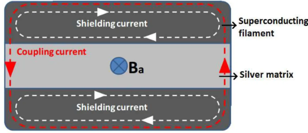
1G tapes, composed by superconducting filaments and a silver matrix, when subjected to variable magnetic fields, produce shielding currents in the superconducting filaments and coupling currents in both, the superconducting regions and the silver matrix. Figure 2.19 depicts the existence and location of this parasitic currents. It is possible to make a separation between these two losses components as well (Rabbers 2001), however that is not the purpose of this work.
Figure 2.19. Shielding and coupling currents in a 1G HTS tape. Adapted from (Ceballos 2010). The magnitude of these losses depend on the resistivity of the silver matrix but also on the time derivative of the magnetic flux across the area between the filaments. This means that the longer the filaments the greater is this area, which results in higher losses (Ceballos 2010).
As demonstrated in (Ishii et al. 1996), these losses can be expressed as shown in equation (2.14):
l d I f
P p
ed
2 2 2 3 02
2
(W/m) (2.14)
In this expression,
0 is vacuum permeability, f is frequency, Ipis current amplitudethrough the tape,
d
is sheath thickness,
is resistivity of silver andl
is perimeter of the outer superconducting filament layer. 2G tapes – eddy currents losses
25 Although the mechanisms that originate these losses in 1G and 2G tapes are different, it is common to designate this component as eddy currents losses in both kinds of HTS tape. 2.2.1.2. Transport current losses
An AC current flowing in a superconductor originates the so-called transport current losses. These can also be divided into three categories:
Self-field losses: originated due to the variation of the magnetic field created by the HTS tape;
Flux-flow losses: due to the movement of the magnetic vortices in the superconductor;
Resistive losses: both, in the superconductor (when close to the critical current) and in the other conductive layers.
The three types of transport current losses can be briefly described as follows.
Self-field losses
When an AC current flows through the HTS tape, it generates a magnetic field, denominated as self-field. This magnetic field originates hysteretic losses similar to those created by an external field presented in the previous section.
Flux-flow losses
Like all type II superconductors, high temperature superconductors usually work in the mixed state. This means that the flux penetrates the superconductor in some specific areas known as vortices. When a transport current is applied, these vortices tend to move towards the boundaries of the superconductor. If the current is sufficiently high, the interaction force surpasses the force pinning the vortex, which will cause the vortex to move through the superconductor dissipating energy (Poole et al. 2007).
Resistive losses
26
2.3.2.
Models of AC losses
In the design phase of a superconducting device project, it is important to model all characteristics of the used superconductors. This will allow saving resources in the implementation phase and find possible sources of difficulties during the project. AC losses must be a part of this project and therefore models for AC losses are often used to obtain results for the total amount of losses in the superconductor. This is extremely important, considering that all generated heat must be extracted from the cryogenic environment where the superconducting device will work. Considering this, a continuous investigation effort has been dedicated in the last decades to achieve accurate models for AC losses in superconductors. This section contains a brief description of the most common models.
2.3.2.1. Analytical models
Analytical models are the most straightforward methods to calculate the total amount of AC losses in superconductors. Even if the models are not too accurate, they can be used to have a first idea of the total amount of losses.
Norris Model
Norris model is the most common analytical model for AC losses in superconducting tapes (samples of tape, not coils). As demonstrated by W. T. Norris in (Norris 1970), hysteretic AC losses of superconducting tapes with an elliptical section can be calculated as:
2
2
1
ln
1
0 2F
F
F
F
I
L
C C
(J/m/cycle) (2.15)
with
C peak
I I
F ,
I
C is critical current.L
C is loss per length of tape per cycle.Even considering that this equation was formulated for low temperature superconductors in 1970 (HTS was not yet discovered), it is accurate for HTS tapes and almost every research group uses it as comparison, when calculating AC losses in samples of HTS tape.
Clem Model
27
Other models
In the last years other analytical models to calculate AC losses not only in samples of HTS tape but also in coils have appeared. (Rabbers et al. 2001) presents an engineering formula that describes AC losses in 1G HTS tape considering a simultaneously applied magnetic field and current (with different orientations). In (Yuan et al. 2009) an extension of the Clem Model is presented, in order to successfully calculate magnetization and transport current AC losses in HTS coils.
One other simple analytical model is that presented in (Pardo 2008). Using as a starting point the Norris model for the calculation of the loss per length of a superconducting slab (equation 34) (Norris 1970), and considering a superconducting coil with internal radius much larger than its width and a high number of turns, the AC loss per tape length can be calculated as:
)
(
6
)
/
(
3 2 2 3 0h
d
I
I
J
d
w
Q
C ap c
(J/m/cycle) (2.16)where
w
,
d
are respectively the width and thickness of the superconducting layer, his the separation between superconducting layers of adjacent turns,J
Cis the critical current density andI
ap/
I
cis the ratio of applied current to the critical current. Equation (2.16) is particularly useful for HTS coils wound using 2G HTS tape, in which the superconducting layer is very narrow comparing to the total dimension of the tape consequently the coil.2.3.2.2. Numerical Models