Abstract
The objective of this work is to provide a reliable numerical model using the finite element method (FEM) for the static and dynamic analysis of reinforced concrete (RC) shells. For this purpose two independently computer programs based on plasticity and visco-plasticity theories are developed. The well known degenerated shell element is used for the static analysis up to failure load, while 3D brick elements are used for the dynamic application. The implicit Newmark scheme with predictor and corrector phases is used for time integration of the nonlinear system of equations. Two benchmark examples analyzed by others are solved with the present numerical model and results are compared with those obtained by other authors. The present numerical model is able to reproduce the path failure, collapse loads and failure mechanism within an acceptable level of accuracy.
Key words
Reinforced Concrete (RC) Shells, Finite Element Method (FEM)
Static and Dynamic Analysis of Reinforced Concrete
Shells
1 INTRODUCTION
Nonlinear analysis of reinforced concrete shells is an important subject nowadays. Thorough inves-tigation of capacity and safety aspects, concrete structures require to establish that the entire struc-tural response up to collapse. For this purpose, mathematical models for predicting the behavior of concrete in static and dynamic loading are presented. Based on plasticity and viscoplasticity theo-ries, such predictions are possible. The finite element method is the natural choice for spatial dis-cretization of complex structural systems. The basic equilibrium and incremental equations for this method are easily obtained using the principle of virtual work. In general, it may be stated that practical problems require insight and understanding in order to develop efficient methods of analy-sis. This paper discusses the development of two different computer programs for the analysis of reinforced concrete structures under static and dynamic loading. The first program is suitable for the static analysis of reinforced concrete shells using the theory of plasticity with the degenerated 9-node shell finite element proposed by Figueiras [4]. The second program handles the dynamic load-ing case usload-ing the theory of viscoplasticity usload-ing the 20-node brick finite element as presented by
Jorg e L. P . Ta ma yo*, a, In ácio B. Mors chb an d Arma nd o M. Awru chb
a CEMACOM, Computational and Applied Mechanical Center, Engineering School, Federal University of Rio Grande do Sul, Av. Osvaldo Aranha, 99-3o Floor, 90035-190, Porto Alegre, RS, Brazil,
b PPGEC, Department of Civil Engineering, Engineering School, Federal University of Rio Grande do Sul, Av. Osvaldo Aranha, 99-3o Floor, 90035-190, Porto Alegre, RS, Brazil,
Received 08 Sep 2012 In revised form 21 Nov 2012
Latin American Journal of Solids and Structures 10(2013) 1109 – 1134
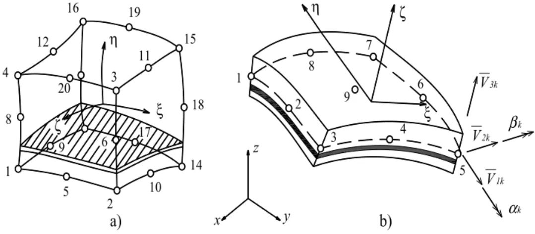
Gomes [5]. In Fig. 1, the two finite elements used in this work are shown. The brick element degen-erates into the shell element when its upper and lower nodes joint together into its middle plane, being both essentially very similar. Also in the same figure, the natural coordinates systems are shown.
Figure 1 Configuration of two layer beam under dynamic loading
2 FINITE ELEMENT FORMULATION
2.1 Finite element formulation and elasto-plastic constitutive model of the degenerated
shell element
The 9-node shell element is used here to represent the concrete shell structure where the reinforcing bars are modeled using the smeared layer approach. The displacement field within the element is defined in terms of quadratic shape functions and displacement values at the nodes. Each nodal point has three degrees of freedom
u
,v
andw
, displacement components along the cartersiancoordinates
x
,y
andz
, respectively and two local degrees of freedomsα
andβ
, which are rota-tions depending on the local coordinate system defined by the nodal vectors{ }
V
1,
{ }
V
2 and{ }
V
3as illustrated in the right side of Fig. 1. The degrees of freedoms
u
andv
are associated to mem-brane actions, whilew
,α
andβ
are associated to bending actions. Therefore, for each elementthe displacement vector is expressed in the following manner:
U
{ }
s=
{
u
1,
v
1,
w
1,
α
1,
β
1,
u
2,
v
2,
w
2...
w
20,
α
20,
β
20}
(1)In addition, several concrete and steel layers are defined through thickness in order to capture properties variations due to nonlinearities. A plane stress assumption coupled with out of plane shear stresses is considered for each layer. Then, the strain components, in the local system of the element are given by:
V2k
V1k
V3k
βk
αk
η ζ
ξ
x y
z
1
2
3 4
5 6 7
8
9
1 8 4
12
16 19
15
18
14
10 2 5
9 6
17
20 3
11
η
ξ ζ
ε
{ }
=
ε
x′ε
y′γ
x′y′γ
x′z′γ
y′z′⎧
⎨
⎪
⎪
⎪
⎩
⎪
⎪
⎪
⎫
⎬
⎪
⎪
⎪
⎭
⎪
⎪
⎪
=
∂ ′
u
∂ ′
x
∂ ′
v
∂ ′
y
∂ ′
u
∂ ′
y
+
∂ ′
v
∂ ′
x
∂ ′
u
∂ ′
z
+
∂ ′
w
∂ ′
x
∂ ′
v
∂ ′
z
+
∂ ′
w
∂ ′
y
⎧
⎨
⎪
⎪
⎪
⎩
⎪
⎪
⎪
⎫
⎬
⎪
⎪
⎪
⎭
⎪
⎪
⎪
+
12
(
∂ ′
w
∂ ′
x
)
21
2
(
∂ ′
w
∂ ′
y
)
2∂ ′
w
∂ ′
x
+
∂ ′
w
∂ ′
y
0
0
⎧
⎨
⎪
⎪
⎪
⎩
⎪
⎪
⎪
⎫
⎬
⎪
⎪
⎪
⎭
⎪
⎪
⎪
=
{ }
ε
0+
{ }
ε
L (2)where,
ε
{ }
0=
ε
x′ε
y′γ
x′y′γ
x′z′γ
y′z′⎧
⎨
⎪
⎪
⎪
⎩
⎪
⎪
⎪
⎫
⎬
⎪
⎪
⎪
⎭
⎪
⎪
⎪
=
[ ]
B
k[ ]
θ
T,
h
2
{
ζ
[ ]
B
k+
[ ]
C
k}
[ ]
θ
TV
{ }
1k{ }
V
2k⎡
⎣
⎤
⎦
⎡
⎣⎢
⎤
⎦⎥
k=1 9
∑
u
kv
kw
kα
1kβ
2k⎧
⎨
⎪
⎪
⎪
⎩
⎪
⎪
⎪
⎫
⎬
⎪
⎪
⎪
⎭
⎪
⎪
⎪
(3) orε
{ }
0=
[ ]
B
s0{ }s
U
(4)where
{ }
V
1k and
{ }
V
2k define the nodal coordinate system at each nodek
of the element (see Fig.1) and matrices[ ]
B
k,
[ ]
θ
and[ ]k
C
are given explicitly in appendix A. In addition,[ ]s
B
0 is the usual strain-displacement element matrix (e.g. see Figueiras [4]). For the degenerate shell ele-ments employed in this work a specific total Lagragian formulation is adopted for modeling geomet-rical nonlinear behavior in which large deflections and moderate rotations are accounted for. Within this approach, the current 2nd Piola Kirchhoff stress tensor components and the Green-Lagrange strain tensor components are referred to the original geometric configuration and the displacement field gives the current configuration of the system with respect to its initial position. Refering varia-bles to the original configuration is advantageous for degenerate shell elements, since the computa-tionally expensive transfer of quantities between local and global axes need to be performed only once. The strain-displacement matrix[ ]
B
s0 is calculated once during the nonlinear process ant its
corresponding nonlinear part
[ ]
B
s1 to be described next is updated using the current displacement
Latin American Journal of Solids and Structures 10(2013) 1109 – 1134
ε
{ }
L=
1
2
(
∂ ′
w
∂ ′
x
)
21
2
(
∂ ′
w
∂ ′
y
)
2∂ ′
w
∂ ′
x
+
∂ ′
w
∂ ′
y
0
0
⎧
⎨
⎪
⎪
⎪
⎩
⎪
⎪
⎪
⎫
⎬
⎪
⎪
⎪
⎭
⎪
⎪
⎪
=
12
[ ]
S
k[ ]
G
kk=1 9
∑
u
kv
kw
kα
1kβ
2k⎧
⎨
⎪
⎪
⎪
⎩
⎪
⎪
⎪
⎫
⎬
⎪
⎪
⎪
⎭
⎪
⎪
⎪
(5)
or
ε
{ }
L=
1
2
[ ]s
B
1{ }
U
s (6)where
[ ]
S
k and
[ ]
G
k are matrices given explicitly in appendix A and contain the contribution of each nodal variable to the local derivates∂ ′
w
∂ ′
x
and∂ ′
w
∂ ′
y
. In addition, several concrete andsteel layers are defined through thickness. Perfect adherence is considered between concrete and steel reinforcement, so Eq. (1) is also valid for steel layers. The stress components of the Piola-Kirchhoff stress tensor for concrete and steel materials in the element local coordinate system are determined by the following expression:
σ
{ }
=
⎡
⎣
σ
x′σ
y′τ
x′y′τ
x′z′τ
y′z′⎤
⎦
T=
[ ]
D
{ }
ε
(7)where
[ ]
D
is the material constitutive matrix in the local coordinate system for a given integrationpoint. The nodal equivalent forces
{ }
P
i and the stiffness element matrix[ ]
K
s i
, at a given iteration
i
, are obtained applying the principle of virtual works and are given by the following expressions:K
[ ]
si
=
[ ]
B
s T
V
∫
[ ]
D
et i
B
[ ]
sdV
+
[ ]
G
T
V
∫
[ ]
σ
[ ]
G
dV
(8)
P
{ }
i=
[ ]
B
s
{ }
σ
i
dV
V
∫
(9)with,
B
[ ]
s=
[ ]
B
s0+
[ ]
B
s1 (10)where
[ ]
D
et i
is the uncracked, cracked or elasto-plastic tangential constitutive matrix for the
stress or geometric stiffness matrix where stress components matrix
[ ]
σ
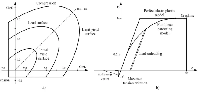
is defined in appendix A. A minimum number of eight concrete layers are found to be suitable for the integration of the above expressions besides a gaussian rule of 2x2 for the middle plane of each layer. Concrete in compression is modeled using the associated theory of plasticity; a modified Drucker-Prager yield criterion, which was proposed by Figueiras [4], is used in this work. Due to nonlinear hardening behavior, this yield criterion defines an initial yield surface at an effective stress equal toσ
0=
0.3f
c (which is the beginning of the plastic deformation) and a limit surface separating a nonlinearstate from a perfect elasto-plastic one, as it is shown in Fig. 2. The yield criterion is defined as:
f
(
σ
)
=
{
1.355
⎣
⎡
(
σ
x2+
σ
y2−
σ
xσ
y)
+
3
(
τ
xy2+
τ
xz2+
τ
yz2)
⎤
⎦
+
0.355
σ
o(
σ
x+
σ
y)
}
1 2
=
σ
o (11)where
σ
0 is the effective stress. In addition, the associated flow rule is defined as:d
ε
ij p
=
d
λ
∂
f
(
σ
)
∂σ
ij
=
{ }
a
T
D
[ ]
e′
H
+
{ }
a
T[ ]
D
e{ }
a
d
ε
{ }
∂
f
(
σ
)
∂σ
ij
(12)
with the flow vector given by:
a
{ }
T=
∂
f
∂σ
x∂
f
∂σ
y∂
f
∂σ
xy∂
f
∂σ
xz∂
f
∂σ
yz⎡
⎣
⎢
⎢
⎤
⎦
⎥
⎥
(13)
In Eq. (8),
{ }
d
ε
contains the components of the total strain,d
ε
ij p
is a component of the plastic
strain tensor,
[ ]
D
e is the elastic constitutive matrix and
H
′
is the hardening parameterestab-lished as the slope of the uniaxial curve which defines the hardening rule. This curve known as “Madrid parabola” is defined by the following expression:
σ
y
=
H
(
ε
p)
=
E
cε
p+
2
E
c2
ε
o
ε
p(
)
1/2 (14)where
E
c is the elastic modulus,
ε
o represents the total strain at cracking compression stressf
c andε
p is the effective plastic deformation. The elasto-plastic constitutive relation is expressed inthe following differential form:
d
σ
{
}
=
[ ]
D
ep{ }
d
ε
=
[ ]
D
e−
[ ]
D
e{ }
a
{ }
a
TD
[ ]
e′
H
+
{ }
a
T[ ]
D
e{ }
a
⎧
⎨
⎪
⎩⎪
⎫
⎬
⎪
⎭⎪
d
ε
{ }
(15)Latin American Journal of Solids and Structures 10(2013) 1109 – 1134
where
[ ]
D
ep is the elasto-plastic constitutive matrix. Finally, the crushing is given by:1.355
ε
x
2
+
ε
y2−
ε
xε
y(
)
+
1.01625
γ
xy
2
+
γ
xz2+
γ
yz2(
)
+
0.355
ε
u
(
ε
x+
ε
y)
=
ε
u2
(16)
where
ε
u represents the ultimate deformation extrapolated from experimental test.
Figure 2 a) Two-dimensional criterion adopted for concrete; b) Uniaxial representation of concrete models
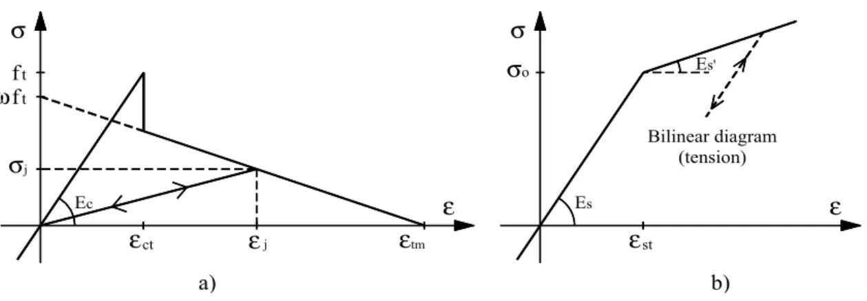
On the other hand, the response of concrete under tensile stresses is assumed to be linear elastic until the fracture surface is reached and then, its behavior is characterized by an orthotropic mate-rial. The cracking is governed by a maximum stress criterion. Cracks are assumed to occur in planes perpendicular to the direction of the maximum tensile stress as soon as this stress reaches the speci-fied concrete tensile strength
f
t. After cracking has occurred the elastic modulus and Poisson’s ratio are assumed to be zero in the perpendicular direction to the cracked plane, and a reduced shear modulus is employed. Due to bond effects, cracked concrete carries, between cracks, a certain amount of tensile force normal to the cracked plane. This effect is considered through a relationship between the strain and the stress normal to the cracking plane direction, as shown in Fig. 3, whereε
ct is the strain associated to
f
t andε
tm is the maximum strain forω
between 0.5-0.7 and thenormal stress
σ
j is determined from a known value of strain
ε
j. Further details of the constitutivemodel for concrete can be found in Figueiras [4]. The steel reinforcement is modeled as an uniaxial elasto-plastic material with a constant elastic steel
E
s and a tangential modulusE
′
s according to the bilinear stress-strain relation shown in the right side of Fig. 3.
σ2 = σ1
a) b)
εU /fc
0.2 0.6 1.0
-0.2
-0.2
0.2 0.6 1.0
σ1
Initial yield surface Load surface
Compression
Tension
Limit yield surface
Crushing
Load-unloading
Softening
curve Maximun tension criterion
Perfect elasto-plastic model
Non-linear hardening
model
ε /fc
σ2
ft 0.3fc
Figure 3 Uniaxial diagram: a) Tension stiffening model; b) Constitutive law for steel
2.2 Finite element formulation and elasto-viscoplastic constitutive model of the 3D brick
element
The 20-node isoparametric quadratic brick element is used here to represent the concrete shell structure where the reinforcement bars are modeled also using the smeared layer approach. The displacement field within the element is defined in terms of the shape functions and displacement values at the nodes. Each nodal point has three degrees of freedom
u
,v
andw
along thecarter-sian coordinates
x
,y
andz
, respectively. Therefore, for each element the displacement vector isexpressed in the following manner:
U
{ }
b=
{
u
1,
v
1,
w
1,
u
2,
v
2,
w
2...
u
20,
v
20,
w
20}
(17)
The strain components vector is defined by:
ε
{ }
=
ε
xε
yε
zγ
xyγ
yzγ
xz⎧
⎨
⎪
⎪
⎪
⎪
⎩
⎪
⎪
⎪
⎪
⎫
⎬
⎪
⎪
⎪
⎪
⎭
⎪
⎪
⎪
⎪
=
∂
N
k∂
x
0
0
∂
N
k∂
y
0
∂
N
k∂
x
0
∂
N
k∂
y
0
∂
N
k∂
x
∂
N
k∂
z
0
0
0
∂
N
k∂
z
0
∂
N
k∂
y
∂
N
k∂
z
⎡
⎣
⎢
⎢
⎢
⎢
⎢
⎢
⎢
⎢
⎤
⎦
⎥
⎥
⎥
⎥
⎥
⎥
⎥
⎥
Tk=1 20
∑
u
iv
iw
i⎧
⎨
⎪
⎩
⎪
⎫
⎬
⎪
⎭
⎪
(18) orε
{ }
b=
[ ]
B
b{ }
U
b (19)
ε
stε
σ
Es a) Es'σ
o Bilinear diagram (tension) b)ε
ct ft ft ωε
σ
Ecσj
Latin American Journal of Solids and Structures 10(2013) 1109 – 1134
where
N
k is the shape function of nodek
and[ ]
B
b is the strain-displacement matrix. The stresses
and strains are related by the following expression:
σ
{ }
b=
⎡
⎣
σ
xσ
yσ
zτ
xyτ
yzτ
xz⎤
⎦
T=
[ ]
D
{ }
ε
b (20)
where is the material constitutive matrix in the global system. Equivalent nodal forces, at a given iteration
i
, are expressed in the following manner:P
{ }b
i=
[ ]
B
b TV
∫
{ }b
σ
idV
(21)The stiffness matrix for a concrete element of volume
V
can be expressed as:K
[ ]
b i=
[ ]
B
b TD
[ ]
iB
[ ]
bdV
V∫
=
[ ]
B
b T
D
[ ]
iB
[ ]
bJ d
ξ
d
η
d
ζ
−1+1
∫
−1
+1
∫
−1
+1
∫
(22)where
J
is the determinant of the jacobian matrix andξ
,η
andζ
represent the local naturalcoordinates at each integration point within the element. As it was mentioned earlier, the steel bars are assumed to be distributed over the concrete element in any direction in a layer with uniaxial properties. A composite concrete-reinforcement constitutive relation is used in this case. To derive such a relation, perfect bond is assumed between concrete and steel. Crushing criteria is similar to that presented in the previous section while the cracking monitoring algorithm presented in Gomes [5] is used.
Earlier developments and studies suggest that a concrete model intended for transient analysis should be rate and history dependent. Apparently, elasto-plastic and elasto-viscoplastic models in their basic formulations do not meet these requirements, but they can be modified to incorporate such effects. However, Cotosvos and Pavlovic [3] have given a detailed explanation for this apparent strength gain at high loading rates. They attribute this fact due to the effect of the inertia loads that reduce the rate of cracking and consequently lead to an increase of the load-carrying capacity of the structure. Therefore, the use of a constitutive model which is dependent on the strain loading rate is questionable. As the objective of this work is not to discuss this issue in detail, the wide ac-ceptance rate and history dependent load model presented by Gomes [5] is still used.
The present model is a strain-rate sensitive elasto-viscoplastic model with progressive degrada-tion of the strength and it introduces two main differences when compared with the tradidegrada-tional elasto-viscoplastic model. Firstly, the fluidity parameter is not constant and it is assumed to be dependent on the elastic strain rate and secondly, a variable strength limit surface is introduced to monitor the damage caused by the viscoplastic flow. If the stress point reaches the strength limit surface, then the degradation of the yield surface is initiated. The yield surface
F
D, defining the onset of viscoplastic behavior, and the strength limit surfaceF
f, defining the initiation of materialdegradation, will be described in terms of first and second invariants only. Both surfaces are ex-pressed in the following manner:
F
D(σ
,σ
o(w
p,
k))
=
cI
1+
c
2I
1 2+
3β
J
2{
}
1 2−
σ
o(w
p,
k)
=
0
F
f(
σ
,
σ
f(w
p))
=
cI
1+
c
2I
12+
3
β
J
2{
}
1 2−
σ
f(w
p)
=
0
(23)
where
I
1 andJ
2 are the first and the deviatoric second stress invariants, respectively. The
con-stants
c
andβ
are evaluated from experimental test and are equal to 0.1775 and 1.355,respective-ly. During inelastic straining both surfaces change, depending on the amount of accumulated dam-age, which is expressed as the viscoplastic energy density
w
p and it is given by:w
p=
σ
Tε
vp
dt
0
t
∫
k
=
w
p−
w
p f=
σ
Tε
vp
dt
tft
∫
(24)
where
t
f andw
pf are, respectively, the time and viscoplastic energy density when the strength limit is reached. While the stress path remains inside the yield surface, the behavior of concrete is linearly elastic, no viscoplastic straining is developed, and the yield and failure surfaces remain sta-tionary. When the stress path is outside the yield surface, inelastic straining occurs, and the values ofσ
o andσ
f vary. Expansion of the yield surface due to hardening is not considered here. How-ever,σ
f decreases with the increase of damage and the strength limit surface shrinks. The strength
limit surface is only a monitoring device to define where and when the failure occurs. When the stress path reaches the strength limit surface, degradation of the material is initiated. After that, the strength limit surface is not longer considered and the yield surface begins to shrink according to the post-failure dissipated energy density
k
. All those paths described before are well depicted inFig. 4.
An exponential function will be used to describe the post-failure behavior. Therefore, the func-tion
σ
o
(w
p,k
)
is defined by the following expression:σ
o(w
p,
k)
=
α
1f
c'w
p≤
w
p fσ
o
(w
p,k
)
=
α
1f
c'
exp(
−α
c
k)
w
p>
w
p f(25)
Latin American Journal of Solids and Structures 10(2013) 1109 – 1134
where
α
1 defines the limit for elastic behavior (typically between 0.3-0.4) and
α
c models thedeg-radation after failure. The parameter
f
c' is the static compressive strength of concrete. The failurestress will be assumed to be a linear function of the viscoplastic energy density and the function
σ
f
(
w
p)
is defined by the following expression:σ
f(
w
p)
=
β
of
c '(1
−
β
1w
p)
0
<
w
p≤
w
p f(26)
Figure 4 Basic concept of the model taken from Gomes [5]
The parameters
β
o andβ
1 are determined from experimental test andβ
of
c' is the compressive
strength obtained with infinite load rates and no inelastic strains. The rate of viscoplastic straining depends on the rate of elastic strain and on the position of the yield surface. It is written as:
ε
=
γ
(
ε
e)
F
Dα
1f
c'∂
f
∂σ
(27)
t = 0 0 < t < tf
The fluidity parameter
γ
(
ε
e)
is related to the elastic strain rate through an exponential func-tion of an effective elastic strain rate.γ
(
ε
e
)
=
a
o(
ε
e eff)
a1 (28)
where
a
o anda
1 are parameters which must be determined experimentally. The effective elastic strain is defined as:
ε
e eff
=
3J
2e(1
+
v)
2{
}
1 2 (29)
because deviatoric strains cause most damage to concrete and
ε
eeff is equal to the uniaxial elastic strain for a uniaxial stress state, beingJ
2e the second invariant of the deviatoric elastic tensor.
3 NUMERICAL ALGORITHM
In order to introduce the implicit numerical algorithm for the solution of the dynamic equation, it is necessary to describe the predictor and corrector form of the Newmark scheme for the integration of the semi-discrete system of equations governing nonlinear transient dynamic problems. Typically at time station
t
n+1 these equations take the following form:
M
[ ]
{ }
a
n+1+
[ ]
C
{ }
v
n+1+
∫
[ ]
B
T{ }
σ
n+1(
d
n+1)
d
Ω
=
f
n+1 (30)where
[ ]
M
and[ ]
C
are the mass and damping matrices while{ }n
a
+1,
{ }
v
n+1 and{ }n
d
+1 are theacceleration, velocity and displacement vectors. The tangential stiffness matrix
[ ]
K
et is related to
the internal forces in the following manner:
[ ]
K
{ }
Δ
d
=
∫
[ ]
B
{ }
+d
+d
Ω
−
∫
[ ]
B
{ }
d
d
Ω
n n T nn T n
et
σ
1(
1)
σ
(
)
(31)with
K
et=
∫
[ ]
B
T[ ]
D
ep[ ]
B
d
Ω
(32)
In the Newmark scheme the displacement and velocity at time
t
n+1 can be expressed in the
fol-lowing form:
d
{ }
n+1=
d
{ }
n+1+
Δ
t
2β
{ }
a
Latin American Journal of Solids and Structures 10(2013) 1109 – 1134
v
{ }
n+1=
{ }
v
n+1+
Δ
t
γ
{ }
a
n+1 (34)with
d
{ }n
+1=
d
{ }n
+
Δ
t v
{ }n
+
Δ
t
2(1 2
−
β
)
{ }n
a
(35)
v
{ }
n+1=
{ }
v
n+
Δ
t
(1
−
γ
)
{ }
a
n (36)Note that
{ }n
d
,{ }n
v
and{ }
a
n are the approximations to
d
(
t
n)
,
d
(
t
n)
andd
(
t
n)
andβ
andγ
are free parameters which control the accuracy and stability of the method.{ }
d
n+1 and
v
{ }
n+1are the predictor values and
{ }
d
n+1 and
{ }
v
n+1 are the corrector values. Initially the displacementsd
{ }
0 and velocities{ }
v
0 are provided and the acceleration{ }
a
0 is obtained from the following expression:M
[ ]
{ }
a
0=
f
0−
[ ]
C
{ }
v
0−
[ ]
K
e{ }
d
0 (37)
By using Eq. (30) to Eq. (36), an effective static problem is formed which is solved using a New-ton Raphson type scheme. This algorithm is summarized in Table 1.
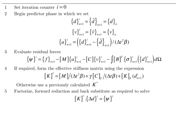
Table 1 Newmark’s algorithm
1 Set iteration counter
i
=
0
2 Begin predictor phase in which we set
d
{ }
n+1 i=
{ }
d
n+1=
d
{ }
nv
{ }
n+1i
=
{ }
v
n+1
=
{ }
v
na
{ }
n+1i
=
{ }
d
n+1 i−
{ }
d
n+1(
)
/ (Δ
t
2β
)
3 Evaluate residual forces
ψ
{ }
i=
{ }
f
n+1−
[ ]
M
{ }
a
in+1−
[ ]
C
{ }
v
in+1−
∫
[ ]
B
T{ }
σ
in+1(
{ }
d
in+1)
d
Ω
4 If required, form the effective stiffness matrix using the expression
K
[ ]
*=
[ ]
M
(
Δ
t
2β
)
+
γ
[ ]T
C
(
Δ
t
β
)
+
[ ]T
K
(
d
n +1i
)
Otherwise use a previously calculated
K
*5 Factorize, forward reduction and back substitute as required to solve
K
Table 1 (continued)
6 Enter corrector phase in which we set
d
{ }
n+1i+1
=
{ }
d
n+1 i
+
{
Δ
d
}
ia
{ }
n+1i+1
=
{ }
d n+1 i−
{ }n
d+1
(
)
/ Δt2β
(
)
v
{ }
in++11=
{ }
v
n
+
Δ
t
γ
{ }
a
n+1 i+17 If
Δ
d
i and/or ψi do not satisfy the convergence conditions then seti
=
i
+
1
andgo to step 3, Otherwise continue 8 Set
d
{ }
n+1=
{ }
d
n+1 i+1v
{ }n
+1=
{ }n
v
+1
i+1
a
{ }
n+1=
{ }
a
n+1 i+1For use in the next time step. Also set n = n+1, form
Cv
n+1
+
B
T
σ
n+1
(
d
n+1)
d
Ω
∫
and begin Next time step
The above algorithm is also useful for static problems by simply omitting all the inertial terms such as the mass and damping matrices and also the velocity and acceleration vectors. In this case the time step is a fictitious time which is used as an incremental multiplier.
4 NUMERICAL APPLICATIONS
4.1 Geometrically nonlinear reinforced parabolic cylindrical shell experimentally tested by
Hedgren and Billington (1967)
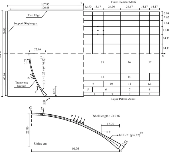
A parabolic cylindrical shell with variable thickness, subjected to uniformly distributed pressure load
P
, which was tested by Hedgren and Billington (see e.g. Figueiras [4]), is analyzed with the present finite element code, which includes a total Lagrangian scheme to analyze geometrically non-linear problems. The shell structure was tested with end support diaphragms and free edges. A fi-nite element mesh of 36 heterosis fifi-nite elements is used to model one quarter of the structure due to symmetry considerations. Material properties are listed in Table 2 and the layout plant and transversal cross section of the shell are shown in Fig. 5. For a detailed description of the layer pat-tern zones of the reinforcement, the reader is referred to the work of Figueiras [4]. Because different amount of reinforcement with different directions are present in various zones of the shell, this ex-ample is considered to be a very challenger case. Then, several steel layers need to be defined for each finite element to take into account space steel variation.Latin American Journal of Solids and Structures 10(2013) 1109 – 1134
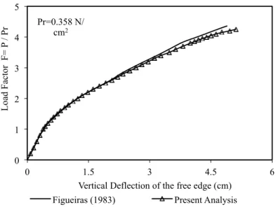
agreement is found at each load level. It is important to explain that all the results presented here are normalized with respect to the results obtained using a reference load
P
r=
0.358
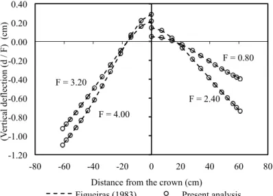
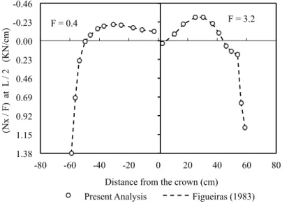
N/cm2. The present numerical model predicts a failure load factor equal to 4.25 while the ultimate experimental load factor was 4.35. The vertical deflections of the transverse section at midspan of the shell are presented in Fig. 7 for load factors of 0.8, 2.4, 3.2 and 4.0. The horizontal displacements at support section are shown in Fig. 8 for load factors 0.4, 2.4 and 4.2. The transverse variation of stress re-sultantsN
x and
M
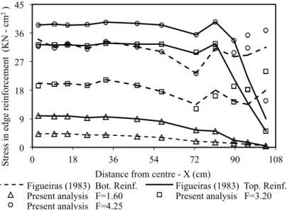
y at midspan are shown in Fig. 9 and Fig. 10 for load factors of 0.4 and 3.2, respectively.Fig. 11 shows the stresses in the main reinforcement along the free edge for three different load levels. The full line corresponds to the bottom reinforcement and the dashed line refers to the rein-forcement top layer. From the difference between the stresses in the top and bottom layer, the mo-ment acting on the free edge can be estimated. It should be noted that the ultimate load has been found before the main reinforcement has reached its ultimate strength. All the previous results shown good agreement with the results reported by Figueiras [4].
Figure 5 Layout plant (with the finite element mesh and the different reinforced patters) and cross section of the parabolic reinforced concrete shell
Free Edge
Support Diaphragm
Transverse Section
Finite Element Mesh
5.08 7.62 8.84
11.16
14.13
14.13
x y
12.50 15.17 24.00 26.67 14.17 14.17 107.95
106.68
60.96
60.96
124
.91
15 16 17
13 14
9 10 11 12
5 6 7 8
1 2 3 4
Layer Pattern Zones
h
= 1
.2
7
+ (
y'
/
6.8
2)
1.5
22.86
1.
27
P
12.70
y'
3.
81
3.81 1.27
CL
22.8
6
60.96 P
Units: cm
y
h=1.27+(y/6.82)3/2 12.70
Table 2 Material properties (cm, KN)
Concrete Steel
Young’s modulus 2069.0 Compressive strength 3.02 Cracking tensile strength 0.48 Poisson ratio 0.20 Uniaxial crushing strain 0.0035 Tensile stiffness parameter 0.5 0.2
Young’s modulus 20000.0 Hardening modulus 4000.0 Yield stress (#3) 25.29 Ultimate stress (#3) 36.42 Yield stress (#4) 21.91 Ultimate stress (#4) 34.49 Yield stress (#9) 30.66 Ultimate stress (#9) 42.00
Figure 6 Load versus vertical displacement of the free edge at the midspan
Pr=0.358 N/ cm2
0 1 2 3 4 5
0 1.5 3 4.5 6
L
oa
d F
ac
tor F
= P
/
P
r
Latin American Journal of Solids and Structures 10(2013) 1109 – 1134
Figure 7 Vertical deflections of the transverse section at the mid-span (x=0)
Figure 8 Longitudinal displacement (x-direction) of the end-supported section
F = 4.00
F = 0.80
F = 2.40 F = 3.20
-1.20 -1.00 -0.80 -0.60 -0.40 -0.20 0.00 0.20 0.40
-80 -60 -40 -20 0 20 40 60 80
(V
ert
ic
al
de
fl
ec
ti
on (d /
F
) (c
m
)
Distance from the crown (cm)
Figueiras (1983) Present analysis
0 4 8 12 16 20 24
-0.024 -0.016 -0.008 0.000 0.008 0.016 0.024
V
ert
ic
al
c
oordi
na
te
Z
(c
m
)
Figure 9 Transverse variation of the stress-resultant Nx at mid-span
Figure 10 Transverse variation of moment My at mid-span
F = 0.4 F = 3.2
-0.46
-0.23
0.00
0.23
0.46
0.69
0.92
1.15
1.38
-80 -60 -40 -20 0 20 40 60 80
(N
x /
F
) a
t L
/
2 (K
N
/c
m
)
Distance from the crown (cm)
Present Analysis Figueiras (1983)
F = 0.40
F = 3.20 -0.20
-0.15
-0.10
-0.05
0.00
0.05
0.10
0 20
40 60
M
y (M
y /
F
) a
t L
/
2 (K
N
- c
m
/
c
m
)
Distance from the crown (cm)
Latin American Journal of Solids and Structures 10(2013) 1109 – 1134
Figure 11 Longitudinal variation of stresses in the main reinforcement along free edge
4.2 Aircraft impact on nuclear power plant (1964)
The horizontal impact of an aircraft on the shield building of a nuclear power plant is analyzed (see Cervera and Hinton [2]). The geometry, the loading function and the reinforcement are specified in Fig. 12. The built-in reinforced concrete shell is composite of cylindrical and spherical parts of con-stant thickness. The reinforcement placed circumferentially and meridionally on the interior and exterior surfaces consist of bars of 40 mm diameter, spaced at 8 cm. The material properties are shown in Table 3. The impact is assumed to occur horizontally and is analyzed following an uncou-pled procedure in which its effect onto the nuclear power plant is considered through the applica-tion of a short-time load (See References [2],[6],[8],[9] and [10]) as shown in Fig. 12. The locaapplica-tion of the area of impact of 28 m2 is also shown in Fig. 12. The load history is also indicated in the same figure and it is noted that the load has a maximum value of 9000 ton.
0 9 18 27 36 45
0 18 36 54 72 90 108
S
tre
ss
i
n e
dge
re
inforc
em
ent
(K
N
- c
m
2 )
Distance from centre - X (cm)
Figure 12 Nuclear containment structure: general layout and loading time history for aircraft impact taken from Cervera et al. [2]
Since the loading and geometry of the shell are symmetric, only one half of the structure is mod-eled. A mesh of 54 solid elements is used in the analysis, with a local refinement in the vicinity of the impact load where a rectangular area of 14 m2 is defined to apply the distributed load (see Fig. 13). The implicit Newmark scheme with
β
=
0.25
andγ
=
0.5
is used to integrate in time with atime step
Δ
t
=
0.00475
. In Table 4, a summary of results for the linear and nonlinear horizontalLatin American Journal of Solids and Structures 10(2013) 1109 – 1134
Abbas et al. [1], whose response greatly differs from that obtained by Cervera and Hinton [2] for a cracking value 0.0015.
Horizontal displacements at points A, B and C are plotted as functions of time in Fig. 14, Fig. 15 and Fig 16, respectively. Two different values of cracking strain are considered here (0.0015 and 0.00185). In order to compared similar profiles of displacements (see Fig. 14), the response obtained using a cracking strain value 0.00185 is compared directly to that obtained by Cervera and Hinton [2] using a cracking value 0.0020 because it yields approximately the same peak displacement at time 0.274s. It is important to emphasize that some differences are expected due to the slightly different mesh used and because of the great sensibility of the response at the impact zone due to cracking. This means that a small variation in the value of the cracking strain could yield signifi-cant changes in displacements. Others facts to take into account in the final response are the sensi-bility established by the type of the integration rule used (an eighteen point selective integration rule was used) and the value of the covering of the reinforcement mesh, which is considered to be 10 cm in this work. Results obtained at point B are also expected to be slightly different because the finite element mesh presents a small circular opening at the upper part of the dome. In general, the profile patterns and magnitude of displacements at the three different locations are in good agree-ment with those presented by Cervera and Hinton [2].
Table 3 Material properties (cm, Kg)
Concrete Steel
Young’s modulus 27000.0 Young’s
modu-lus 20000.0
Compressive strength 350.0 Yield strength 29.5
Cracking tensile strength variable Fluidity param-eter
a0 = 1.539
a1 = 0.971
Poisson ratio 0.20
Uniaxial crushing strain 0.0035
Mass density 0.245E-05
Fracture energy 0. 2
Fluidity parameter 0.3055
Yield surface function a1 = 0.40
ac= 10.0
Failure surface function b0 = 1.84
Table 4 Peak displacement and elastic modulus for concrete used by different authors (cm, Kg)
Concrete Elastic modulus
for concrete
Peak displacement
(some authors could have reported point A)
Elastic Nonlinear
Crutzen and Reyne [10] Rebora and Zimmermann [10]
Cervera and Hinton [2] Abbas et al. [1] Pandey et al. [10]
Kubreja [8] Madasamy et al. [9]
Iqbal et al. [6] Liu [7] Gomes [5] Present analysis not given not given 30000.0 30000.0 30000.0 not given not given 27386.0 30000.0 20000.0 27000.0 4.08 3.63 2.98 3.14 3.5 not given 4.0 not given 2.89 3.68 2.85 4.47 4.29 2.98 to 5.8 3.14 to 3.60 3.50 to 4.00
4.60 4.20 6.69 3.11 to 4.48
3.70 2.85 to 5.90
a)
b)
c)
Figure 13 Finite element mesh with 54 brick elements a) Plant view; b) Isometric view; c) Deformed mesh.
Figure 14 Horizontal displacement of point A for different cracking strain values with fracture energy equal to 0.2Kg/cm.
-2000 -1500 -1000 -500 0 500 1000 1500 2000 0 200 400 600 800 1000 1200 1400 1600 1800 2000 X -10 0 1000 0 1000 0 1000 2000 3000 4000 5000 6000 -2000 -1000 0 1000 2000 0 1000 0 1000 2000 3000 4000 5000 6000 2 1 Present analysis 3 -6 -4 -2 0 2 0.00 0.12 0.24 0.36 0.48 0.60
D is pl ac em ent of poi nt A (c m ) Time (s) (1) Elastic
(2) Crack strain 0.00185 (3) Crack strain 0.0015
1 2 3 Cervera & Hinton (1987) -6 -4 -2 0 2 0.00 0.12 0.24 0.36 0.48 0.60
D is pl ac em ent of poi nt A (c m ) Time (s) (1) Elastic
Latin American Journal of Solids and Structures 10(2013) 1109 – 1134
Figure 15 Horizontal displacement of point B for different cracking strain values with fracture energy equal to 0.2Kg/cm.
Figure 16 Horizontal displacement of point C for different cracking strain values with fracture energy equal to 0.2 Kg/cm.
5 CONCLUSIONS
In this work, the usual elasto-plastic and elasto-viscoplastic algorithms are used to predict the dy-namic and static behavior of reinforced concrete shells. Validation of the present algorithms and codes are provided by modeling two usual benchmark examples found in the technical literature about this topic. These two examples are considered to be complex because of the nonlinearities involved and in the case of the static example also due to the complex reinforcement arrangement. For the dynamic analysis of the nuclear power plant, different results (even for the linear case) are reported in the literature by various authors. Then, some explanations are given to justify these differences such as that the final response is very sensitive to the way in which cracking develops within the impact zone, the location of the peak displacement and the value of the elastic modulus of concrete. Several tests have shown that mesh refinement near the impact zone, time step value
2
Present analysis
1
3 -4
-2.4
-0.8
0.8
0.00 0.12 0.24 0.36 0.48 0.60
D
is
pl
ac
em
ent
of poi
nt
C (c
m
)
Time (s) (1) Elastic
(3) Crack strain 0.0015 (2) Crack strain 0.00185
Cervera & Hinton (1987)
3 2
1 -4
-2.4
-0.8
0.8
0.00 0.12 0.24 0.36 0.48 0.60
D
is
pl
ac
em
ent
of poi
nt
C (c
m
)
Time (s) (1) Elastic
(2) Crack strain 0.0020 (3) Crack strain 0.0015
1 2
3
Present analysis -4
-2.4
-0.8
0.8
0.00 0.12 0.24 0.36 0.48 0.60
D
is
pl
ac
em
ent
of poi
nt
B (c
m
)
Time (s) (1) Elastic
(3) Crack strain 0.0015 (2) Crack strain 0.00185
1 Cervera &
Hinton
(1987) 2
3 -4
-2.4
-0.8
0.8
0.00 0.12 0.24 0.36 0.48 0.60
D
is
pl
ac
em
ent
of poi
nt
B (c
m
)
Time (s) (1) Elastic
for the dynamic analysis and covering value of the reinforcement mesh have little influence in the final results.
Otherwise, because the elasto-viscoplatic algorithm is explicit, a suitable time step size must be chosen for the stability of the integration of the constitutive relations. This time step size is related to the specific form of the viscoplastic potential used in the flow rule. In addition, the global stabil-ity of the procedure also depends on the time step length chosen for the integration of the dynamic equation of motion. These dependencies make the elasto-plastic algorithm more attractive because automatic sub-incrementation can be used instead of selecting a suitable time step size for the inte-gration of the constitutive relations. In this way, the procedure is reduced only to the choice of a suitable time step length for the integration of the dynamic equation of motion. Finally, results obtained here are in good agreement with those numerically obtained by other authors. Further investigation is carried out to implement a strain rate sensitive elasto-plastic model for concrete and also to include other effects such as concrete creep and shrinkage.
Acknowledgments The financial support provided by CAPES and CNPQ is gratefully acknowl-edged.
References
[1] H. Abbas, D.K. Paul, P.N. Godbole, and G.C. Nayak. Aircraft crash upon outer containment of nuclear power plant. Nuclear Engineering and Design, 160(1):13-50, 1996.
[2] M. Cervera and E. Hinton. Análisis dinámico en rotura de estructuras laminares y tridimensionales de hormigón armado. Rev. Internacional de Métodos Numéricos para Calculo y Diseño en Ingeniería, 3(1):61-76, 1987.
[3] D.M. Cotsovos and N. Pavolic. Numerical investigation of concrete subjected to compressive impact load-ing. Part1: A fundamental explanation for the apparent strength gain at high loading rates. Computers and Structures, 86(1-2):145-163, 2008.
[4] J.A. Figueiras. Ultimate load analysis of anisotropic and reinforced concrete plates and shells, PhD. Thesis, University of Wales, U.K., 519, 1983.
[5] H. Gomes, 1997, Análise da confiabilidade de estruturas de concreto armado usando o método dos elemen-tos finielemen-tos e processos de simulação, Dissertação de Mestrado, Universidade Federal do Rio Grande do Sul, 1997.
[6] M.A. Iqbal, S. Rai, M.R. Sadique, and P. Bhargava. Numerical simulation of aircraft crash on nuclear con-tainment structure. Nuclear Engineering and Design, 243:321-335, 2012.
[7] G.Q. Liu. Nonlinear and transient finite element analysis of general reinforced concrete plates and shells, PhD. Thesis, University of Wales, U.K., 1985.
[8] M. Kukreja. Damage evaluation of 500 MWe Indian pressurized heavy water reactor nuclear containment for aircraft impact. Nuclear Engineering and Design, 235(17-19):1807-1817, 2005.
[9] C.M. Madasamy, R.K. Singh, H.S. Kushwaha, S.C. Mahajan, and A. Kakodkar. Nonlinear transient analy-sis of Indian PHWR reinforced concrete containments under impact load – A case study. Transactions of the 13th International Conference on Structural mechanics in Reactor Technology (SMIRT), H038-1:243-248, 1995.
Latin American Journal of Solids and Structures 10(2013) 1109 – 1134
Appendix A
For a given node
k
, the following expressions apply:[ ]
[ ]
⎥
⎥
⎥
⎥
⎥
⎥
⎦
⎤
⎢
⎢
⎢
⎢
⎢
⎢
⎣
⎡
=
⎥
⎥
⎥
⎥
⎥
⎥
⎦
⎤
⎢
⎢
⎢
⎢
⎢
⎢
⎣
⎡
=
2 1 3 1 3 2 2 3 2 3 1 3 1 2 2 10
0
0
0
0
0
0
0
0
0
0
0
0
0
C
C
C
C
C
C
C
C
C
B
B
B
B
B
B
B
B
B
k k (A1)B
1=
∂
N
k∂
ξ
A
11+
∂
N
k
∂
η
A
12C
1=
N
kA
33B
2=
∂
N
k∂
ξ
A
21+
∂
N
k
∂
η
A
22C
2=
N
kA
23B
3
=
∂
N
k∂
ξ
A
31+
∂
N
k∂
η
A
32C
3=
N
kA
13(A2)
A
11A
12A
13A
21A
22A
23A
31A
32A
33⎡
⎣
⎢
⎢
⎢
⎤
⎦
⎥
⎥
⎥
=
[ ]
θ
T[ ]
J
−1=
[ ]
θ
T∂ξ
∂
x
∂η
∂
x
∂ζ
∂
x
∂ξ
∂
y
∂η
∂
y
∂ζ
∂
y
∂ξ
∂
z
∂η
∂
z
∂ζ
∂
z
⎡
⎣
⎢
⎢
⎢
⎢
⎢
⎢
⎢
⎤
⎦
⎥
⎥
⎥
⎥
⎥
⎥
⎥
(A3)where
![Figure 4 Basic concept of the model taken from Gomes [5]](https://thumb-eu.123doks.com/thumbv2/123dok_br/18884684.423540/10.892.304.647.210.725/figure-basic-concept-model-taken-gomes.webp)