No 659 ISSN 0104-8910
An Ordering of Measures of the Welfare Cost
of Inflation in Economies with
Interest–Bearing Deposits
Os artigos publicados são de inteira responsabilidade de seus autores. As opiniões
neles emitidas não exprimem, necessariamente, o ponto de vista da Fundação
An Ordering of Measures of the Welfare Cost of
Inflation in Economies with Interest-Bearing
Deposits
∗
Rubens Penha Cysne
†David Turchick
‡EPGE - Funda¸c˜ao Getulio Vargas
December 3, 2007
Abstract
This paper builds on Lucas (2000) and on Cysne (2003) to derive and or-der six alternative measures of the welfare costs of inflation (five of which al-ready existing in the literature) for any vector of opportunity costs. The or-dering of the functions is carried out for economies with or without interest-bearing deposits. We provide examples and closed-form solutions for the log-log money demand both in the unidimensional and in the multidimen-sional setting (when interest-bearing monies are present). An estimate of the maximum relative error a researcher can incur when using any particular measure is also provided.
∗Key Words: Inflation, Welfare, Interest-Bearing Assets, Money Demand, Divisia Index. JEL:
C0, E40.
†Professor at the Graduate School of Economics of the Getulio Vargas Foundation
(EPGE/FGV). E-mail: [email protected].
1
Introduction
Measuring the welfare costs of inflation, even when restricted to a money-demand
approach (e.g. [1], Lucas (2000), Simonsen and Cysne (2001), and Cysne (2003)),
presents the researcher with at least four types of problems.
First, choosing among the several welfare measures existing in the literature
and being reasonably aware of the consequences of this choice for the maximum
possible relative error of the welfare figures to be obtained.
For instance, Lucas (2000) derives a measure of the welfare costs of inflation
based on the Sidrauski model and another one based on the shopping-time model.
He shows, using numerical simulations, that both Sidrauski’s and the
shopping-time measures are very close to Bailey’s (1956) measure. However, he does not
provide, either analytically or numerically, an ordering among such three functions
of the nominal interest rate. A researcher might want to know how such measures
compare to each other (if they can be ordered) and, moreover, what would be
the consequences (the maximum relative error, for instance) for the welfare figures
obtained using any particular measure.
A second problem a researcher might face is the necessity to take into
con-sideration the existence in the economy of interest-bearing deposits performing
monetary functions. This leads us, as conjectured by Lucas (2000, p. 270) and
later shown by Cysne (2003), to welfare measures based on Divisia indices of
monetary services. Using the unidimensional welfare formulas in this case can be
misleading, particularly because the demand for non-interest-bearing money can
be very sensitive to variations in the opportunity costs of other assets providing
The same way as different unidimensional formulas can be defined, different
Divisia indices can be used to calculate welfare losses in the multidimensional
setting. Once again, the question of how such welfare measures relate to each other
emerges, but now in a more complicated fashion. Knowing in advance that some
measures always lead to welfare figures that are higher (or lower) than others, for
any vector of opportunity costs, is again valuable information for those interested
in investigating the losses generated by inflation.
Answers to such questions have been provided in the literature by
Simonsen and Cysne (2001) and by Cysne (2003), but only in relation to four
measures of the welfare costs of inflation: Lucas’ shopping-time measure, two
(easier-to-calculate) approximations of Lucas’ measure introduced by Simonsen
and Cysne (2001) and Bailey’s measure.
This paper extends such contributions, both in the unidimensional and in the
multidimensional case, by reconsidering the previous ordering with respect to two
additional measures: Lucas’ measure based on Sidrauski’s model, which he derives
taking as reference the interest rate currently prevailing in the economy; and a
measure which is new in the literature, the one which emerges from Sidrauski’s
model when the reference for income compensation is taken to be an interest rate
equal to zero.
The paper also contributes to the related literature by providing with respect
to the usual log-log money demand:
i) closed-form solutions to all six measures, both in the unidimensional and in
the multidimensional setting;
any of the six different measures;
iii) numerical examples illustrating the main results of the paper.
The remainder of the paper is organized as follows. In section 2 we present
the results concerning the unidimensional case worked out by Lucas (2000).
Start-ing with the unidimensional case is didactically important because it provides the
reader, in a more simplified setting, a reference for the steps which are to be taken
in the multidimensional case. Section 3 exemplifies the results of the
unidimen-sional case and provides an order of magnitude of the maximum relative error.
Sections 4 and 5 extend the previous results of Sections 2 and 3 to the case in
which the existence of interest-bearing deposits performing monetary function is
taken into consideration. Section 6 summarizes the paper.
2
Six alternative measures of the welfare costs
of inflation
In this section we analyze the case of an economy with only one type of (non
interest-bearing) money. We present the six alternative measures of the welfare
cost of inflation we shall deal with and show how they can be ordered. By ”show
how they can be ordered” we mean that we shall demonstrate that these six
2.1
The shopping-time measure and its approximations
Lucas (2000, p. 265) shows that in the shopping-time model the welfare cost of
inflation s is given as a solution to the non-separable differential equation:
s′(r) = −rm′
(r)
1−s(r)+rm(r)(1−s(r)) s(0) = 0
, (1)
wherer ∈R+ stands for the nominal interest rate andm : [0,+∞]→[0,+∞] is a
money-demand function that arises from the model itself.
Since the non-separable differential equation given by (1) does not have any
obvious solution in the general case,1 it is natural to look for approximations to
it. Simonsen and Cysne (2001) have shown that reasonable approximations to s
in (1) are given by the upper bound A:R+→[0,+∞]:
A(r) :=
Z r
0
− ρm
′(ρ)
1 +ρm(ρ)dρ. (2)
and by the lower bound 1−e−A.
Let B :R+→[0,+∞] stand for Bailey’s (1956) measure:
B(r) :=
Z r
0
−ρm′
(ρ)dρ. (3)
Through the transformation µ:=m(ρ), (2) and (3) can be rewritten as
A(r) =
Z m(0) m(r)
ψ(µ)
1 +µψ(µ)dµ (4)
1Cysne (2005) has provided a solution to it in the case of a log-log money demand. This
and
B(r) =
Z m(0) m(r)
ψ(µ)dµ, (5)
where this last formula is the traditional one for the area under the inverted
money-demand curve.
Simonsen and Cysne (2001) have also shown that
1−e−A< s < A < B, (6)
where we write ”f < g” for ”f(r) < g(r),∀r ∈ R++”, since all these measures
coincide only at 0. This notation will be used for the ordering of functions.
2.2
The Sidrauski model
In the next subsection we will introduce two measures of the welfare cost of inflation
which emerge from the Sidrauski model. Both are based on Lucas’ version of this
model, and since one of them is new in the literature, we present the model here
in detail. Another reason for doing so is that later on we will want to generalize
this model, so that it also accounts for the possibility of existence of other types
of monies in the economy.
Let’s assume a forever-living perfectly-foresighted representative agent
max-imizing a time-separable constant-relative-risk-aversion utility function, the
ar-guments of which are the flows of real consumption of a single non-monetary
nonstorable good and the holdings of real cash balances.
For every t ∈ [0,+∞), let Bt ∈ R+, Mt ∈ R+, Ht ∈ R, Yt ∈ R++ and
bonds and cash, a lump-sum tax (if negative, a transfer from the government to
the individual), nominal output and consumption at timet. The budget constraint
faced by our representative agent is:
˙
Bt+ ˙Mt=Yt−Ht−Ct+rtBt,
where the dots mean time-derivatives and rt ∈R+ stands for the nominal interest
rate bonds yield at time t (by definition, cash is a monetary asset always yielding
a nominal interest rate of 0).
Let Pt ∈ R++ be the (both expected and realized) price level, πt:=
˙
Pt
Pt be the inflation rate at time t, and γ stand for the constant rate of output growth:
y(t) =y0eγt. (7)
Lower-case variables are real counterparts of the above nominal variables as
frac-tions of output (that is, bt := BYtt etc.).
As in Lucas (2000), we assume the utility function to be homogeneous of degree
1−σ, in which case we can use (7) (normalizing y0 to be equal to one) to write
our agent’s problem (PS) as
max
ct,mt≥0
Z +∞
0
e(−ρ+(1−σ)γ)tU(c
t, mt)dt (PS)
subject to
˙
bt+ ˙mt=yt−ht−ct+ (rt−πt−γ)bt−(πt+γ)mt
Note that, in (PS), the representative agent is supposed to perform her
maxi-mization over real consumption and real cash balances, and not over these variables
as fractions of the output. Following Lucas (2000), we use an instantaneous utility
function U :R+×R+→[−∞,+∞] with the functional form:
U(c, m) = 1
1−σ
cϕm c
1−σ
,
where σ > 0, σ 6= 1, extended to the ray {0} ×R+ by continuity. ϕ : [0,+∞] →
[0,+∞] is a twice-differentiable function. We assume that there is an ¯m∈(0,+∞]
such that ϕ |[0,m¯) is strictly increasing and strictly concave and ϕ |[ ¯m,+∞] is
con-stant.2
Remark 1 The expression ϕ(m)−mϕ′(m) will appear many times throughout
this work, so it should be noted from the start that, for positive m, this expression
is positive. Indeed, for m < m¯, the strict concavity of ϕ gives ϕ(0) −ϕ(m) <
ϕ′(m)(0−m), and since ϕ(0) ≥ 0, we have ϕ(m)−mϕ′(m) > 0. For m ≥ m¯,
ϕ(m)−mϕ′(m) =ϕ( ¯m)>0.
Notice that U is strictly increasing in each of its variables and also strictly
concave.3 Therefore, assuming that (P
S) has a solution, it will be unique. Using
2It will turn out to be the maximum value the money-demand function arising fromϕ and
(PS) attains. For example, for the log-log money-demand specification m = Kr−α, we would
have ¯m= +∞, whereas for the semi-log specificationm=Ke−αr,m=K.
3All we need to check is that, for (c, m)∈
R2++,
Uc(c, m) = cϕ mc−σ
ϕ mc
−m cϕ′
m c
>0,
Um(c, m) = cϕ m
c −σ
ϕ′ m
c
>0,
Ucc(c, m) = cϕ m
c
−σ−1
−σ ϕ m c −m cϕ ′ m c 2
+m2 c2 ϕ
m c
ϕ′′ m
c
<0,
Umm(c, m) = cϕ mc−σ−1−σϕ′ mc2+ϕ mcϕ′′ mc<0,
Ucm(c, m) = cϕ mc−σ−1
σmcϕ′ m
c 2
−ϕ mc
σϕ′ m
c
+m cϕ′′
m c
, and
Ucc(c, m)Umm(c, m)−Ucm(c, m)2= −σ
c3 cϕ
m c
1−2σ
ϕ′′ m
c
the budget constraint to substitute for c, we get a standard calculus of variations
problem in the variables b and m. The Euler equations are:
(r−π)Uc = (−ρ+γ(1−σ))U +dtd(−Uc)
−πUc+Um = (−ρ+γ(1−σ))U +dtd(−Uc)
.
Since the right-hand sides of these equations are the same, we at once obtain
the very intuitive equilibrium relation
r = Um
Uc
. (8)
In equilibrium, sincecis taken as a fraction of output,c= 1. Equation (8) can
then be rewritten as:
r= ϕ
′(m)
ϕ(m)−mϕ′(m), (9)
which corresponds to equation 3.7 in Lucas (2000) (which he derives using
Bell-man’s Optimality Principle instead). This equation gives us r as a non-negative
differentiable function ofm, for which we shall writer=ψ(m), whereψ : [0,m¯]→
[0,+∞].
Note that equation (9) may be rewritten as:
ϕ′
(m) = ψ(m)
1 +mψ(m)ϕ(m), (10)
which is separable and yields the general solution
ϕ(m) =CeR1m ψ(µ)
for some constant C >0.
In the steady state the Euler equation relative to b gives
r =ρ+π+γσ, (12)
a fact that justifies our taking of the welfare cost of inflation as a function of the
nominal interest rate, instead of inflation itself.
Since
ψ′
(m) = ϕ(m)ϕ ′′(m)
(ϕ(m)−mϕ′(m))2 <0, (13)
ψ is strictly decreasing, therefore one-to-one. From its continuity (sinceϕ is
twice-differentiable, ϕ′ is continuous), its image is also connected, that is, an interval
[ψ( ¯m), ψ(0)]. From (9), we haveψ( ¯m) = 0. LetR:=ψ(0).
We shall call ψ’s inverse function m : [0, R] →[0,m¯] a ”money-demand
func-tion”. This function is strictly decreasing (m′(r) = 1
ψ′
(m(r)) < 0) and surjective
by construction. As a practical matter, since the economist does not know the
function ϕ, he ends up using a money-demand function estimated by the
econo-metric practice, implying restrictions that have to be satisfied by ϕ (the so-called
”integrability problem” in economics).
2.3
The welfare cost of inflation in the Sidrauski model:
two different approaches
In Sidrauski’s framework, Lucas (2000, p. 257) ”define[s] the welfare cost w(r)
of a nominal rate r to be the percentage income compensation needed to leave
interpreting this definition. The first one, employed by Lucas, uses the initial
interest rate as reference and measures the percentage rise in income necessary to
make people as well off as they would be if the nominal interest rate were to fall
to zero. Given the 1-degree homogeneity of U one can simply write:
U(1 +w(r), m(r)) =U(1,m¯). (14)
Let ϕ∗ := sup
m>0ϕ(m) = ϕ( ¯m). From (11), we then have
ϕ∗
=CeR1m¯ ψ(µ) 1+µψ(µ)dµ
so that ϕ∗ < +∞ if and only if the integral Rm¯
1
ψ(µ)
1+µψ(µ)dµ converges (this is an
issue if ¯m = +∞).
In our framework, (14) implies:
(1 +w(r))ϕ
m(r) 1 +w(r)
=ϕ( ¯m) = ϕ∗
. (15)
Differentiating with respect to r, dividing through by ϕ′ m(r)
1+w(r)
and using
(10):
w′
(r) = −ψ
m(r) 1 +w(r)
m′
(r). (16)
This is equation 3.11 in Lucas’ paper which, together with the conditionw(0) = 0,
enables us to find w.
We will now turn our attention to another natural way of interpreting Lucas’
definition for the welfare cost of inflation in Sidrauski’s model: the one which
welfare cost of inflation the percentage fall in the representative agent’s income
that would make her as well off as she would have been, had no increase in the
nominal interest rate taken place:
U(1, m(r)) =U(1−w(r),m¯). (17)
We shall see below that the welfare cost of inflation which takes as reference an
interest rate equal to zero (w) is lower than the one which takes as reference the
prevailing (supposedly positive) interest rate (w). Bailey’s measure lies somewhere
in between4. This will be proved in Proposition 1 below.
In our model, definition (17) implies:
ϕ(m(r)) 1−w(r) =ϕ
¯
m
1−w(r)
. (18)
Now, since, by construction, w(r)∈[0,1), we have m¯
1−w(r)) ≥m¯, so that
ϕ
¯
m
1−w(r)
=ϕ∗ ,
and (18) ends up yielding the very simple formula for the welfare cost of inflation
w:
w(r) = ϕ
∗−ϕ(m(r))
ϕ∗ . (19)
4Note that the inequalities presented in (6) as well as all others obtained throughout this paper
In either case (ϕ∗ <+∞ orϕ∗ = +∞), using (4) we may write
ϕ(m(r))
ϕ∗ =
CeR1m(r) ψ(µ) 1+µψ(µ)dµ
CeR+
∞
1
ψ(µ) 1+µψ(µ)dµ
=eR+m∞(r) ψ(µ)
1+µψ(µ)dµ =e−A(r). (20)
Taking into account (19), we obtain:
w(r) = 1−e−A(r). (21)
In Simonsen and Cysne (2001) and in Cysne (2003), the measure 1−e−A has
been derived in a completely different context (the shopping-time one) as an
easier-to-calculate approximation to s, the welfare measure derived by Lucas, given in
(1). Here, we’ve just seen that a different model, the money-in-the-utility-function
model, can provide a sensible explanation to this measure.
Comparing (21) with (16), we see thatwhas at least one advantage over Lucas’
measure w: computational ease. We no longer have to solve a non-separable
nonlinear differential equation – although we do still need to evaluate a possibly
very difficult integral.
Proposition 1 below offers the main result of this Section.
Proposition 1 Let m : [0, R] → [0,m¯] be a differentiable and strictly decreasing
money-demand function, so that we can use it to calculate s, A, B, w, and w (by
simply plugging it into (1), (2), (3), (16) and (21)). Then we have the following
inequality chain:
w= 1−e−A< s < A < B < w.
Proof. The equality has just been shown. The first, second and third inequalities
may notice that their proof that 1−e−A< s < A < B draws only on the strict
de-creasingness ofm, not on other possible characteristics enjoined by money-demand
functions arising from the shopping-time model. As to the fourth inequality, (16)
gives us, forρ∈(0, r],w′
(ρ)>−ψ(m(ρ))m′(ρ) = −ρm′(ρ) (remember thatm′ <0
and that ψ is a strictly decreasing function), so all that is left to do is integrate
both sides of this last inequality.
3
Some calculations for the unidimensional
log-log money demand
3.1
Formulas for the unidimensional measures of the
wel-fare cost of inflation
Let’s say an estimated unidimensional log-log money demand specification,
m=Kr−α, (22)
with K > 0 and α ∈ (0,1), has been handed to us by the econometrician. How
can we calculate the different measures of the welfare cost of inflation associated
to a nominal interest rate ofr?
Fortunately, s has already been calculated in the literature (see Cysne 2005)
for this particular case, being given in an implicit manner by the formula:
(1−s(r))1−(1−s(r))−1/α+ K 1−αr
Both Bailey’s measure and the proxy measure A are straightforward:
B(r) =
Z r
0
−ρ(−αKρ−α−1)dρ= αK
1−αr
1−α (24)
and
A(r) =
Z r
0
−ρ(−αKρ−α−1)
1 +ρKρ−α dρ=α
Z r
0
Kρ−α
1 +Kρ1−αdρ
= α
1−α
Z 1+Kr1−α
1
du
u =
α
1−αlog 1 +Kr
1−α
. (25)
Regarding w, since ψ(m) = Km1/α
, (16) takes the form
w′
(r) =−
K(1 +w(r))
Kr−α
1/α
(−αKr−α−1) =αK(1 +w(r))1/αr−α,
leading to:
w(r) =−1 + 1−Kr1−ααα−1 . (26)
You may notice that in order for w to be real, it’s important that r∈[0, Kα1−1].
Finally, for the welfare measure associated to the compensating variation
no-tion, we simply have:
w(r) = 1−e−A(r) = 1− 1 +Kr1−ααα−1 . (27)
In Figure 1 we plot these five measures for the estimated money-demand
func-tion m(r) = 0.05r−0.5.5 Note how s and A are indistinguishable to the naked
eye.
5These parameters were calibrated so as to fit the American economy. See Lucas (2000, pp.
Figure 1: Welfare Costs in the Unidimensional Case
0 0.2 0.4 0.6 0.8 1 1.2 1.4 1.6 1.8 2
0 0.01 0.02 0.03 0.04 0.05 0.06 0.07 0.08
nominal interest rate
welfare cost of inflation
Another way of finding w would be to first ask what is the ϕ underlying the
money-demand handed out to us, and then use (20). Looking at equation (11),
we first calculate the integral that appears there:
Z m 1 K µ 1/α
1 +µK
µ
1/αdµ= Z m
1
K1/α
µ1/α +K1/αµdµ= Z m 1 dµ µ − Z m 1
µα1−2
K1/α+µα1−1dµ
= logm− α
1−α
Z K1/α+m
1 α−1
K1/α+1
du
u = log
m
,
K1/α+mα1−1 K1/α+ 1
!1−αα
.
Therefore that equation gives us
ϕ(m) = Cm
K1/α+m1−αα
1−αα, (28)
for a positive constant C.6 Soϕ∗ =C, and
w(r) = 1− ϕ(m(r))
ϕ∗ = 1−
m(r)
K1/α+m(r)1−αα
1−αα
= 1− Kr
−α
K1−ααK+K 1−α
α rα−1
1−αα = 1−
1
(Kr1−α+ 1)1−αα,
which coincides with the previous result.
3.2
The maximum relative error
A question that could naturally arise from looking at Figure 1 is: ”How much
greater can the Sidrauski-Lucas upper bound w be relatively to the lower bound
w?”. For reasonable interest rates, not much greater indeed.
From (26) and (27):
∆(r) := w(r)−w(r)
w(r) =
−1 + −1+(1−Kr1 −α
)αα−1
1−(1+Kr1−α
)αα−1 if r >0
0 if r= 0
.
Write
f(x) =
−1 + −1+(1−x) α α−1
1−(1+x)αα−1 if x >0
0 if x= 0
,
so that
∆(r) =f(Kr1−α).
With the aid of a mathematics software, the following third-order Maclaurin’s
expansion forf can be obtained:
f(x) = 0 + 1
1−αx+
1 2(1−α)2x
2+−2α2+ 5α−5
12(1−α)3 x
3 +O(x4),
where O(x4) means a function whose absolute value is less than a constant times
x4, for small enough values ofx(we’re only interested in reasonable interest rates,
which correspond to low x’s).
We want to have ∆(r) written as a function ofw(r). In order to do this, take
g :R+→R given by
g(x) = 1
α
−1 + (1−x)αα−1
Its third-order Maclaurin’s expansion is:
g(x) = 0 + 1
1−αx+
1 2(1−α)2x
2+ 2−α
6(1−α)3x
3+O(x4).
Therefore, for small x, we have
f(x) =g(x) +O(x3).
Note that
g Kr1−α
= 1
αw(r),
so that, by putting x=Kr1−α, we get:
∆(r) = 1
αw(r) +O(r
3−3α), (29)
which is a good approximation to this relative difference formula.
By comparing the dotted and the full line in Figure 2, which cannot be
distin-guished by the naked eye, one can see that the approximation of ∆(r) by 1
αw(r)
is very good indeed. Figure 2 also allows us (again, using a value of K = 0.05),
in relation to three possible alternative values of the interest-rate elasticity α, to
enter an interest rate in the abscissa and to have an idea of the maximum relative
error regarding the use of one or another of the six welfare measures we deal with
in this paper. The upper part of Figure 2 has r ranging from 0 to 1, and is more
appropriate for low-inflation economies. The bottom of Figure 2 gives the same
data when r varies between 0 and 10.
Figure 2: Maximum Relative Error
0 0.5 1
0 0.01 0.02 0.03 0.04 0.05 0.06
maximum relative error
0 0.5 1
0 0.02 0.04 0.06 0.08 0.1 0.12
nominal interest rate
0 0.5 1
0.2 0.25 0.3 0.35 0.4 0.45 0.5 0.55 0.6 0.65 0.7 real difference approximation
alpha=0.1 alpha=0.5 alpha=0.9
0 5 10
0 0.1 0.2 0.3 0.4 0.5 0.6 0.7
maximum relative error
0 5 10
0 0.05 0.1 0.15 0.2 0.25 0.3 0.35 0.4
nominal interest rate
0 5 10
0.2 0.3 0.4 0.5 0.6 0.7 0.8 0.9 1 real difference approximation
of the nominal interest rate could account for an inflation rate around 11% plus a
long-term real interest rate around 4%. It could be understood as an upper bound
for most industrialized economies. Thus, if one reports having found a welfare
loss of, say, 1% of output associated with a money demand having a 0.5 elasticity
and an 11% inflation rate, our results allow us to say that, regardless of which
particular measure among the six was chosen, the estimate could vary at most
between 0.96% and 1.04%, a very reasonable confidence interval. So one can feel
secure about which measure to take, when considering low-inflation countries.
However, the preceding calculations tell only one side of the story. Consider
now a country where the annual inflation rate has reached 400% (in Brazil, for
instance, yearly inflation reached 1783% in 1989). For the same parameters, the
relative measuring difference ∆ reaches 22% (considering r = 4, since the
long-term real interest rate becomes negligible). For example, estimates of the welfare
costs reported as being of 8% of output in high-inflation countries could actually
be measured as low as 6.5% or as high as 9.8%, depending on the formula being
used. In such high-inflation cases, therefore, one has to be careful about which
measuring strategy to pursue.
4
The presence of interest-bearing monies in the
economy
In this section we extend all results obtained in section 2 to a framework in which
n types of monies are available. This is important because, as we argued in the
there are different assets in the economy performing monetary functions. The
variables defined below will be used both in the case of the Sidrauski and the
shopping-time models.
Let
m= (m1, . . . , mn)∈[0,+∞]n
represent the vector of real quantities of each type of money being demanded, as a
fraction of nominal GDP (wherem1 is chosen to bem, real currency per output).
Each mi yields a nominal interest rate ofri, and
r:= (r1, . . . , rn)∈Rn+
(with r1 = 0, by definition). We shall write
u:= (r, r−r2, . . . , r−rn)∈Rn+
for the vector of opportunity costs of holding each type of money instead of
gov-ernment bonds.
The steady-state interest rate r in this extended model is determined by (12),
as in the unidimensional case. The other interest rates r2, ..., rn (as well as the
respective opportunity costs u2, ..., un) can be assumed to be determined by a
competitive and costless banking system subject ton−1 exogenous
non-interest-bearing reserve requirements k2, ...kn (in which case r2 = (1−k2)r, ..., rn = (1−
The reader may verify that:
r= 0 ⇐⇒u =0. (30)
Expressions (30) and (12) show how each of the opportunity costs ui relates
to the rate of inflation. When the nominal interest rate is equal to zero, all the
opportunity costs are also equal to zero and inflation generates no welfare loss at
all. The converse is also true.
The first-order conditions of the money-in-the-utility-function model, as well
as of the shopping-time model, will imply a functionψ takingmintou, analogous
to the functionψ from section 2.
But it is important to keep in mind that from this section on all measures of
the welfare cost of inflation will be evaluated at m, rather than atu. To keep the
notation uniform, though, we will use the same symbols we’ve been using so far
to denote each of the six n-dimensional welfare measures.
4.1
The shopping-time measure and its approximations in
the multidimensional case
The multidimensional McCallum-Goodfriend (1987) model is introduced and solved
in Cysne (2003). There, a transacting-technology constraint in the form
c=G(m)f(s)
is assumed, where cand s stand for the real level of consumption and the portion
G : [0,+∞]n → [0,+∞] is a twice-differentiable 1-degree homogeneous concave
function such that Gxi > 0, limmi→0Gxi(m) = +∞, limmi→+∞Gxi(m) = 0,
Gxixi < 0 for all i ∈ {1, . . . , n},
7 and f : [0,1] → R
+ is a twice-differentiable
function such thatf′ >0 and f′2−f f′′≥0.8
This model’s first-order conditions imply the equilibrium relations (Cysne 2003,
p. 224):
ui = G(mf()sf)′
(s)Gxi(m),∀i∈ {1, . . . , n}
G(m)f(s) = 1−s
.
This last equation, Gf(s) = 1−s, can be seen to give us s as a function of G
alone. For this purpose, we only need to check that the function H : (0,1]→R+
defined by
H(s) = 1−s
f(s)
is invertible. SinceH′(s) = −f(s)−(1−s)f′
(s)
f(s)2 <0,H(1) = 0 and lims→0+H(s) = +∞,
we’re done. By writing τ for its inverse function, the preceding set of equations
becomes a money-demand specification of n variables and n equations:
ui =ψi(m) =
f(τ(G(m)))
G(m)f′(τ(G(m)))Gxi(m),∀i∈ {1, . . . , n}, (31)
whereψi is the i-th component of the functionψ : [0,+∞]n→[0,+∞]n taking m
7Ifn= 1,Gwould have to be linear, whenceG′′= 0. Therefore, our analysis in this section
is restricted to the casen >1. Even so, it yields exactly the same results as then= 1 framework analyzed in section 2.
8This impliesf f′
to be a decreasing function, a fact we shall use soon. In the unidimensional case, this is a sufficient condition (weaker thanf′′≤0) for the money demand which emerges from
into u. In vector notation, we have
u=ψ(m) = f(τ(G(m)))
G(m)f′(τ(G(m)))∇G(m) . (32)
Remark 2 Along rays starting at the origin, each ψi is strictly decreasing. In
fact, if k > 1, we get, by G’s strict increasingness in each variable, G(km) >
G(m). Therefore, since τ is strictly decreasing (likeH), τ(G(km))< τ (G(m)),
and ff′
(τ(G(km))) < ff′
(τ(G(m))). From G’s homogeneity, we also get
Gxi(km) =Gxi(m).
9 Therefore
ψi(km) =
1
G(km)
f f′
(τ(G(km)))Gxi(km)
< 1 G(m)
f f′
(τ(G(m)))Gxi(m) = ψi(m),
as we wished.
The multidimensional analog of (1) was derived in Cysne (2003, eq. 14):
sxi(m) = −
ψi(m)
1−s(m) +ψ(m)·m(1−s(m)). (33)
Consider aC1pathχ: [0,1]→[0,+∞]n
such thatχ(0) = +∞:= +∞(1, . . . ,1)
and χ(1) =m, and the following 1-forms in [0,+∞]n:
dA:=− 1
1 +u·mu·dm (34)
and
dB :=−u·dm. (35)
The line integrals
A(m) :=
Z χ
dA (36)
and
B(m) :=
Z χ
dB (37)
extend Simonsen and Cysne’s (2001) proxy measure to s(2) and Bailey’s measure
(3) to the present framework.10 In Cysne (2003, prop. 1), it is shown that when
ψ arises from the shopping-time model, these integrals are path-independent, so
that A and B are indeed well-defined.
From Remark 2, we see that the initial condition that a welfare-cost function
w(such ass,A orB) has to satisfy in this multidimensional framework is w(d) =
0,∀d ∈ [0,+∞]n \Rn
+ (as mentioned in the beginning of this section, now our
welfare-cost functions are functions of the vector of monetary aggregates, rather
than the interest rates). This is how we get the lowest possible values for theui’s,
which is the benchmark used for measuring the welfare cost of inflation (see (30)).
In proposition 2 of Cysne (2003), it is demonstrated that, exactly as happens
in the unidimensional case, we have
1−e−A < s < A < B.
In the next subsection, we shall introduce the multidimensional analogs of w
and w, and prove that they relate to the above welfare measures in exactly the
same way as in the unidimensional case.
10These are, in order, the additive inverses of the Divisia indicesDE(χ) andDG(χ) presented
4.2
The extended Sidrauski model
Our representative agent’s instantaneous utility will now have the form:
U(c,m) = 1
1−σ
cϕ
G(m)
c
1−σ
,
where σ and ϕ are exactly as in subsection 2.2 (so that ϕ has an ¯m ∈ (0,+∞]
associated to it), and G is exactly as in the previous subsection. Assuming again
real output growth to be equal to γ, her maximization problem will be:
max
ct>0,mt≥0
Z +∞
0
e(−ρ+(1−σ)γ)tU(c
t,mt)dt (PnS)
subject to
˙
bt+1·m˙t=yt−ht−ct+ (rt−πt−γ)bt+ (rt−(πt+γ)·1)·mt
b0 >0 andm0 >0 given.
where we write1for the vector (1, . . . ,1)∈Rn,‘·’ for the canonical inner product of
Rn, and all the non-bold letters have the same meaning as in the model introduced in subsection 2.2.
Considering only regular solutions and substituting for cas we’ve done before,
we may rewrite our maximization problem as
max
b>0,m≫0
Z +∞
0
e(−ρ+(1−σ)γ)tU(y−h+(r−π−γ)b+(r−(π+γ)·1))·m−b˙−1·m,˙ m)dt.
(Pn
The Euler equations are:
(r−π−γ))Uc = (−ρ+γ(1−σ))U + dtd(−Uc)
(ri −π−γ)Uc+Uxi = (−ρ+γ(1−σ))U +
d
dt(−Uc),∀i∈ {1, . . . , n}
,
which really correspond to the optimum of (Pn
S), by U’s concavity.11 As before,
these equations immediately imply
r−ri =
Uxi
Uc
,∀i∈ {1, . . . , n}. (38)
In equilibrium, we have c= 1, so that (38) gives
ui =ψi(m) =
ϕ′(G(m))
ϕ(G(m))−G(m)ϕ′(G(m))Gxi(m),∀i∈ {1, . . . , n}, (39)
where now ψ :G−1([0,m¯])→ [0,+∞]n, G−1 denoting the inverse image of [0,m¯]
under G. Equation (39) is analogous to (9), giving us a differentiable function ψ
taking m intou.
We can rewrite (39) as
u=ψ(m) =F (G(m))∇G(m) , (40)
whereF : [0,+∞]→[0,+∞] is a differentiable and strictly decreasing function (as
already calculated in (13)). The reader may want to notice that this general form
for multidimensional money-demand specifications also encompasses specifications
11Let V stand for the function U of section 2 (of only two variables), so that U(c,m) =
V(c, G(m)). Givenc, d∈R++ andx,y∈Rn+, we have
U(d,y)−U(c,x) =V(d, G(y))−V(c, G(x))≤DcV(c,G(x))(d−c)+DmV(c,G(x))(G(y)−G(x))≤
DcV(c,G(x))(d−c) +DmV(c,G(x))DGx(y−x) = DU(c,x)(d−c,y−x), where we’ve used the
originating from the shopping-time model, given by (32).
We shall now see that the welfare-measures A and B are well-defined also for
money-demand functions arising from the multidimensional
money-in-the-utility-function model. Here, the only difference to the last subsection is that the pathχ
should be such that χ(0)∈G−1({m¯}), and our boundary condition for a generic
welfare-measure w is thatw(d) = 0,∀d ∈G−1({m¯}).12
Lemma 1 If u is given by (40), the line integrals in (36) and (37) are
path-independent .
Proof. All we need to do is check that the 1-forms dA and dB are closed. We
start by the latter.
From (40), we have
(ui)xj(m) =F′(G(m))Gxj(m)Gxi(m) +F (G(m))Gxixj(m) ,
evidently symmetric in (i, j). Therefore, −(ui)xj =−(uj)xi, and dB is closed.
Now for the path-independence of A. Since
1 1 +u·mui
xj
= 1
(1 +u·m)2
h
(1 +u·m) (ui)xj−ui
uj+Pnk=1mk(uk)xj i
,
and we already know that (ui)xj = (uj)xi, it suffices to check that
Pn
k=1mkui(uk)xj is symmetric in (i, j). Using the above expression for (ui)xj and (40), we find
Pn
k=1mkui(uk)xj =
Pn
k=1mkF Gxi F ′
GxjGxk +F Gxkxj
,
12This generalizes perfectly the analysis carried out in the last subsection, where the
which is symmetric in (i, j) iff Gxi
Pn
k=1mkGxjxk is symmetric in (i, j). And this is the case, since this expression actually equals zero, fromGxj’s 0-homogeneity and
Euler’s formula for homogeneous functions.
4.3
The welfare cost of inflation in the extended Sidrauski
model: two different approaches
Let us now write down the equations defining the measureswandwof the welfare
cost of inflation:
U(1 +w(m), G(m)) =U(1,m¯) or
(1 +w(m))ϕ1+Gw(m(m))
=ϕ( ¯m) = ϕ∗;
(41)
U(1, G(m)) =U(1−w(m),m¯) or
ϕ(G(m)) = (1−w(m))ϕ m¯ 1−w(m)
= (1−w(m))ϕ∗.
(42)
Partially differentiating the first of these equations with respect to xi, and
dividing through byϕ′G 1
1+w(m)m
, we obtain:
wxi(m)
ϕG 1
1+w(m)m
ϕ′G 1
1+w(m)m
+
Gxi(m)−wxi(m)G
1
1 +w(m)m
= 0.
But (39) gives us
ϕG 1
1+w(m)m
ϕ′G 1
1+w(m)m
=
Gxi(m)
ψi
1 1+w(m)m
+G
1
1 +w(m)m
so that we get the expression
wxi(m) =−ψi
1
1 +w(m)m
, (43)
analogous to (16).
From ψi’s strict decreasingness along rays starting at the origin, we have
wxi(m) < −ψi(m). Besides this, because of G’s increasingness in every
direc-tion, it is always possible to choose d ∈ G−1({m¯}) such that d ≫ m. Consider
then a path χas in the previous subsection such that χ(0) =d. Therefore:
w(m) =
Z 1
0 d
dλw(χ(λ))dλ=
Z 1 0 −ψ 1
1 +w(χ(λ))χ(λ)
· ∇χ(λ)
dλ
>
Z 1
0
[−ψ(χ(λ))· ∇χ(λ)]dλ =
Z χ
−ψ(µ)·dµ=B(m), (44)
where the first equality follows from the Fundamental Theorem of Calculus and
the condition w(d) = 0; and the inequality sign follows from realizing that since
the leftmost and the rightmost extremities of the above inequality are independent
of χ (Lemma 1), and we took d≫ m, we can consider without loss of generality
that χ is strictly decreasing in every direction.
Let us now turn our attention tow. We have already seen in (42) thatw(m) =
ϕ∗
−ϕ(G(m))
ϕ∗ . On the other hand, writing dG(m) =∇G(m)·dmand using the fact that G(χ(0)) = ¯m, (34) gives
A(m) =
Z χ
−ϕ
′(G(µ))
ϕ(G(µ))dG(µ) =
Z G(m) ¯
m
−ϕ
′( ˜G)
ϕ( ˜G)d ˜
G
=
Z ϕ(G(m))
ϕ∗
−dϕ˜
˜
ϕ = log
ϕ∗
ϕ(G(m))
so
ϕ(G(m))
ϕ∗ =e
−A(m)
. (45)
Therefore we have obtained a perfect analog to (21):
w(m) = 1−e−A(m). (46)
The measuresw andw were introduced for Sidrauski’s model, and were shown
to relate in a precise way with other measures. We are now ready to state and
prove our main ordering result, extending Proposition 1 to an economy with many
types of monies.
Proposition 2 Let ψ :G−1([0,m¯])→[0,+∞]n be a money-demand specification
taking the general form (40) (for instance, one arising from the extended
shopping-time or Sidrauski model), so that we can use it to calculate s, A, B, w, and w
(by simply plugging it into (33), (36), (37), (43) and (46)). Then we have the
following inequality chain:
w= 1−e−A< s < A < B < w.
Proof. It has been proved in Cysne (2003, p. 236) that 1−e−A< s < A < B, in
case we take our pathχso that d
dt∇χ≪0 – and, as we’ve seen above in the proof
of inequality (44), this can always be done. The equality between w and 1−e−A
has been proved in (46). Now it’s only a matter of gluing the inequalities and the
5
Formulas for the Multidimensional Welfare
Mea-sures
Repeating the procedure used in the unidimensional case, in this section we
exem-plify with a multidimensional extension of the log-log money-demand specification
the ordering of the welfare measures given in Proposition 2.
By observing (22) and (40), it is natural enough to propose an extension of the
unidimensional log-log money-demand specification of the form:
ψ(m) =
K G(m)
1/α
∇G(m) ,
where K > 0 and α ∈ (0,1). This is the demand that would emerge from (Pn
S)
and (28).
It is worth noticing that, in the case of G being a weighted geometric mean,
G(m1, . . . , mn) = Qni=1mβii (where βi ≥ 0, ∀i ∈ {1, . . . , n} and Pni=1βi = 1), we
obtain the system
ψ1(m) = K1/αβ1
m1
Qn j=1m
(1−α1)βj
j
...
ψn(m) = K
1/αβ n
mn
Qn j=1m
(1−α1)βj
j
,
which, inverted,13 gives a demand in the format:
m1(u) = L1Qnj=1uα1j
j
...
mn(u) = LnQnj=1uαjnj
,
13The very name of this kind of demand is a hint to how to invert this system of equations:
where theαij’s are the demand elasticities of type iof money with relation to the
opportunity cost of holding type j.
Again, B and A can be easily obtained. Taking χ as in the previous section,
and such that χ(0) = +∞:= +∞(1, . . . ,1) (we may do that since ¯m= +∞), we
have:
B(m) =
Z χ
−ψ(µ)·dµ=−K1/α
Z χ
∇G(m)·dm G(m)1/α
=−K1/α G(m) 1−α1
1−α1
m +∞ = αK 1/α
1−α G(m) 1−α1
, (47)
and
A(m) =
Z χ
−ψ(µ)·dµ
1 +ψ(µ)·µ =−
Z χ
K1/αdG(m)
G(m)1/α+K1/αG(m).
Notice how this is exactly the same integrand that appeared in our second
approach to finding w in the unidimensional case. With that knowledge behind
us, we can immediately write:
A(m) = lim
G∗→+∞
" Z G∗
G(m)
dG˜
˜
G −
α
1−α
Z K1/α+G∗
1 α−1
K1/α+G(m)α1−1
dG˜
˜
G
#
= lim
G∗
→+∞log
G∗
K1/α+G∗α1−1
α 1−α
K1/α+G(m)α1−1
1−αα
G(m)
= log
K1/α+G(m)α1−1
1−αα
G(m)
=
α
1−αlog
1 +K1/αG(m)1−1α
.
(48)
increasing in each variable and 1-homogeneous function, it is unbounded:
lim
m→+∞G(m) = +∞.
Then (48) and (46) give at once:
w(m) = 1−1 +K1/αG(m)1−α1
−1−αα
. (49)
Now for w. Equation (43) takes, in this case, the form:
wxi(m) =−(1 +w(m))
1/α K
G(m)
1/α
Gxi(m) ,
which, as in the unidimensional case, gives
Z w(m)
0
dν
(1 +ν)1/α =−K
1/α Z
χ
∇G(m)·dm
G(m)1/α =B(m) ,
so that
1 1−α1
(1 +w(m))1−α1 −1
= αK
1/α
1−α G(m) 1−α1
,
and
w(m) =−1 +1−K1/αG(m)1−α1
αα−1
. (50)
Finally, for s, the easiest thing to do is just imitate (23) in the obvious way,
and verify that it satisfies (33). That is, take s given implicitly by equation
where
D(m, s) := K
1/α
1−αG(m) 1−α1
+ (1−s)1−(1−s)−1/α.
The Implicit Function Theorem gives
sxi(m) = −
(∂D/∂xi) (m, s(m))
(∂D/∂s) (m, s(m)) =
1
αK1/αG(m)
−1/α
Gxi(m)
−1 + 1− α1
(1−s(m))−1/α
= ψi(m)
−1 + (1−α)1−(1−s(m))−1/α ,
whence
− 1
sxi(m)
= 1
ψi(m)
−
(1−α)1−(1−s(m))−1/α
K1/αG(m)−1/α
Gxi(m) .
Substituting from (51), we get
− 1
sxi(m)
= 1
ψi(m)
+ K
1/αG(m)1−1α
K1/αG(m)−1/α
Gxi(m) (1−s(m))
= 1
ψi(m)
+ G(m)
Gxi(m) (1−s(m)) ,
an expression equivalent to (33). The reader may wish to check that these formulas
really extend the unidimensional ones.
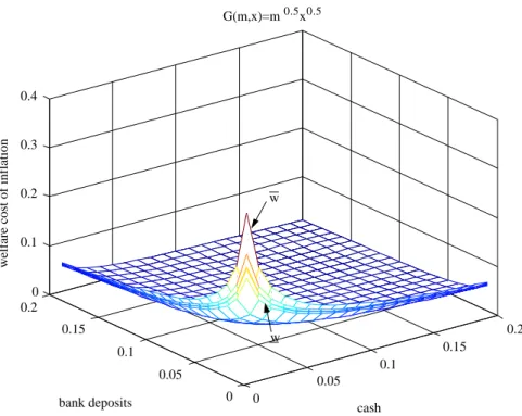
All these measures are plotted in Figures 3 and 4, where n = 2, K = 0.05 and
α = 0.5. In Figure 3, G is taken so that G(m, x) = m0.5x0.5, and in Figure 4,
G(m, x) =m0.7x0.3. The ordering of the surfaces is the one implied by Proposition
2. Again, as in the unidimensional case, we see thatAapproximatessso well that
Figure 3: Welfare Costs in the Multidimensional Case
0
0.05
0.1
0.15
0.2
0 0.05 0.1 0.15 0.2
0 0.1 0.2 0.3 0.4
cash G(m,x)=m0.5x0.5
bank deposits
welfare cost of inflation
w
w
Figure 4: Welfare Costs in the Multidimensional Case
0
0.05
0.1
0.15
0.2
0 0.05 0.1 0.15 0.2
0 0.1 0.2 0.3 0.4
cash G(m,x)=m0.7x0.3
bank deposits
welfare cost of inflation
w
6
Conclusion
The present work has extended the ordering of measures of the welfare costs of
inflation provided by Cysne (2003) to include two new measures derived from
Sidrauski’s money-in-the-utility-function framework. The first measure is provided
by Lucas (though only in relation to the unidimensional case). The second measure
is new in the literature (both for the unidimensional and the multidimensional
case).
The main result of the paper, given in Proposition 2, is the ordering of six
different measures of the welfare costs of inflation both when there is only one type
of money and in the case where there are several interest-bearing assets performing
monetary services.
We have also illustrated our results with the well-known log-log money-demand,
both in the unidimensional and in the multidimensional case. In the presence
of only one type of money we have shown that for parameter values as those
usually found in the literature, the greatest possible relative error a researcher can
incur by deciding to use a particular measure is extremely low in normal scenarios
(only 4% for annual nominal interest rates as high as 15%), but may be high in
hyperinflations (22% if this interest rate is around 400%).
Finally, we have provided closed-form solutions to all six measures of the welfare
costs of inflation both for the unidimensional and the multidimensional framework
References
[1] Bailey, Martin. J. (1956): ”Welfare Cost of Inflationary Finance,” Journal of
Political Economy, 64, 93-110.
[2] Cysne, Rubens P. (2003): ”Divisia Index, Inflation, and Welfare,” Journal of
Money, Credit and Banking, 35, 221-238.
[3] Cysne, Rubens P. (2005): ”A General-Equilibrium Closed-Form Solution to
the Welfare Costs of Inflation,” Revista Brasileira de Economia, 59, 209-214.
[4] Lucas, Robert E., Jr. (2000): ”Inflation and Welfare,”Econometrica, 68,
247-274.
[5] McCallum, Bennett T., and Marvin S. Goodfriend (1987): ”Demand for
Money: Theoretical Studies,” in The New Palgrave: A Dictionary of
Eco-nomics, ed. by John Eatwell, Murray Milgate, and Peter Newman. London:
Macmillan; New York: Stockton Press, 775-781.
[6] Sidrauski, Miguel (1967): ”Rational Choice and Patterns of Growth in a
Mon-etary Economy,” American Economic Review, 57, 534-544.
[7] Simonsen, Mario H., and Rubens P. Cysne (2001): ”Welfare Costs of Inflation
and Interest-Bearing Deposits,” Journal of Money, Credit and Banking, 33,