Measures of the welfare cost of inflation: a complete ordering

Fundação

Getulio

Vargas

Escola

de

Pós-Graduação

em

Economia

Measures

of

the

Welfare

Cost

of

Inflation:

A

Complete

Ordering

David

Turchick

Orientador:

Rubens

Penha

Cysne

Dissertação submetida à Congregação da Escola de Pós-Graduação em Economia (EPGE-FGV)

para a obtenção do grau de

Mestre

em

Economia

Rio de Janeiro, Brasil

Measures of the Welfare Cost of In‡ation:

A Complete Ordering

David Turchick

Advisor: Rubens Penha Cysne

EPGE - Fundação Getulio Vargas

July, 2007

Abstract

This paper presents three contributions to the literature on the welfare cost of in‡ation. First, it introduces a new sensible way of measuring this cost - that of a compensating variation in consumption or income, instead of the equivalent variation notion that has been extensively used in empirical and theoretical research during the past …fty years. We …nd this new measure to be interestingly related to the proxy measure of the shopping-time welfare cost of in‡ation introduced by Simonsen and Cysne (2001). Secondly, it discusses for which money-demand functions this and the shopping-time measure can be evaluated in an economically meaningful way. And, last but not least, it completely orders a comprehensive set of measures of the welfare cost of in‡ation for these money-demand speci…cations. All of our results are extended to an economy in which there are many types of monies present, and are illustrated with the log-log money-demand speci…cation.

1

Introduction

The debate over whether and to what extent we should be concerned about in‡ation has very likely been around since the invention of in‡ation itself. In‡ation, in its turn, is as old as money.1 _{Nevertheless,}

human civilization would have to wait until the second half of the twentieth century, with the rise of modern economic science, to see rigorous and logical attempts at measuring in‡ation’s burden on society. According to Fischer (1981, p. 17), an anticipated 10% in‡ation rate implies a loss of 0.3% of the GNP. More recent …gures (see, for instance, Lagos and Wright 2005, p. 478) are much more dramatic, going as high as 4.1%. If this value were uniformly distributed throughout society, it would mean about $1,000 a year for someone whose annual earnings were $24,000 – most de…nitely a considerable amount. But even if this cost were only 0.3%, it certainly could not be regarded as negligible – for the American economy, for example, it would represent about US$ 40 billion.

In general terms, the problem with in‡ation is that it taxes the holding of real balances, making people spend more of some other real resource instead, and obtain a lower utility level. At least three major approaches to measuring this welfare cost of in‡ation have been advocated: the welfare "triangle" (Bailey 1956), the comparison of steady states (Cooley and Hansen 1989) and the shopping time (Lucas 2000), the

I am extremely grateful to Professor Cysne for sharing so many great ideas with me and for having encouraged me all the way through. I’m also very thankful to Professors Humberto Moreira, Rogério Sobreira and Luiz Henrique Braido for their invaluable suggestions as to the organization of the text, and to my father, Arnold Turchick, for checking the English.

…rst two being the most popular in applications. Depending on how money is introduced in our model, one or another measure becomes the most natural choice.

In the absence of distortionary taxes, Friedman (1969, pp. 33-4) showed that the optimal in‡ation rate is minus the real interest rate, that is, the rate corresponding to a zero nominal interest rate. That is because this rate equates the privately perceived cost of holding one additional dollar (the foregone nominal interest rate this dollar would yield if used to buy a government bond instead) to the social cost of providing it – idealistically, nothing at all. This environment in which the Friedman rule is valid is used as a benchmark in the …rst two measuring strategies mentioned above.

Bailey’s welfare triangle, the area under the inverted money-demand curve, has been calculated in many di¤erent models. Barro (1972) …nds a loss associated to a 10% annual in‡ation rate, in terms of gross national product (this will be the case for all the estimates shown below), of 2.2%.2 _{According to}

Fischer’s (1981) calculations for the U.S. economy, such an in‡ation rate would correspond to a loss of 0.3% of GNP, while Lucas (1981), using similar parameters, …nds 0.45% (p. 43). The main di¤erence is that Fischer considers high-powered money only, while Lucas uses M1. Aiyagari, Braun and Eckstein (1998), motivated by evidence that in‡ation boosts the relative size of the banking sector in the economy, use this size as their de…nition for the welfare cost of in‡ation, and show that it equals Bailey’s measure (p. 1290). They estimate a loss equivalent to 2.0% of GNP (…g. 6, p. 1298).

The second approach to calculating the welfare cost of in‡ation is to address the question: "By how much should we raise an individual’s consumption level so that she would be as happy as if she lived in a world with an optimal in‡ation rate?". Assuming that government expenditures are …nanced by non-distortionary taxes only (which will be the case in this paper), and callingEr the environment in which

the nominal interest rate isr, we could restate this question as: "How much would the equivalent variation in consumption be, as a function of r, when we move from Er to E0?".

In Cooley and Hansen’s (1989) model, in which money enters via a cash-in-advance constraint, in‡ation makes people substitute leisure for consumption, lowering their output and utility level. The above ques-tion is answered for both the M0 and M1 de…niques-tions of money (with monthly and quarterly constraints, respectively), and the estimates found are 0.11% and 0.39% of GNP (table 2, p. 743). In ·Imrohoro¼glu (1992), money is held as a form of insurance against unemployment, allowing a risk-averse agent to smooth his consumption schedule. She answers the same question with a 1.07% estimate (using M0), and also calculates the welfare triangle measure as being 0.41% (p. 88).

Dotsey and Ireland (1996) present a model in which in‡ation distorts the consumption decision in other ways than in Cooley and Hansen’s model. Here, in‡ation also causes people to divert resources from goods production into the …nancial sector, and can a¤ect the growth trajectory as well. For the welfare measure arising from the equivalent variation notion, they …nd estimates associated to a 10% in‡ation rate of 1.8% and 3.9% (table 1, p. 39), depending if the monetary aggregate considered is M0 or M1.3 _{They also}

calculate the Bailey measure, for both money de…nitions (table 2, p. 41): 0.65% for M0 and 0.44% for M1. For the shopping-time measure, Lucas (2000, p. 265) notes that the shopping-time variable in McCal-lum and Goodfriend’s (1987) model may be naturally seen as a measure of the welfare cost of in‡ation itself. This variable represents the fraction of time spent transacting rather than producing, so that, in equilibrium, by economizing on the use of money because of in‡ation, the individual spends more time transacting, and produces and consumes less (as we shall see in subsection 3.1). His estimate for the welfare loss associated to a 10% in‡ation rate is 1.8% of the American GNP (see …g. 8, p. 266).4

2_{Making an average of the costs associated to a 0.5% and a 1% monthly in‡ation, which are 2.0% and 2.4% (values}

presented on table 2, p. 986).

3_{Since they normalize the welfare cost of in‡ation to equal zero when the in‡ation rate is zero, and not when the nominal}

interest rate is zero, we have to subtract the entry in the …rst column from the entry in the fourth column of that table.

4_{The relevant nominal interest rate is 13%, if we choose 3% as the long-term real interest rate (as Lucas does on page 252}

The just-mentioned …gure in Lucas’s paper presents the shopping-time measure as lying always under the Bailey measure, and this is shown to be in fact the general case in Simonsen and Cysne (2001). Moreover, by looking at ·Imrohoro¼glu’s and Dotsey and Ireland’s estimates above, one may conjecture that Bailey’s measure is always lower than the equivalent variation measure, and we shall see in the present work that this also is true.

The reader should note that the usual "comparing-steady-states" measure seems to go in only one direction. There is a natural companion question to the one stated with the equivalent variation notion, that reads: "How much would thecompensating variation in consumption be, as a function of r,when we move from Er to E0?". In other words, "By how much should we decrease an individual’s consumption level so that she would be as happy as if she lived in a world with a positive nominal interest rate?". The answer to this question gives a measure of the welfare cost of in‡ation that is not at all traditional in the literature – although we should not claim that it is new.

In Williamson (1998) – the only paper we were able to track down that uses this compensation notion – the welfare loss associated to in‡ation is due to ine¢ciencies in the credit system. There it is said that "the welfare costs to each type of agent [risk-averse and risk-neutral] [...] are measured in a conventional way" (p. 561), and it seems that the author has Cooley and Hansen’s measuring strategy in mind. But he goes on to de…ne the welfare measure for these agents making use of the compensating variation notion, rather than Cooley and Hansen’s equivalent variation notion. This can be seen as an additional reason (but probably not as important as the ones given in that paper) for the costs he estimates being "an order of magnitude lower than the costs calculated by Cooley and Hansen" (p. 563), since this paper is going to show that the welfare measure associated to the compensating variation notion is always smaller than the one associated to the equivalent variation notion.

Another question that might arise from looking at the estimates given above is: "After all,what is the monetary aggregate we should use to measure in‡ation and its burden on society?". Although we shall not address this question, we do give a su¢ciently general framework so that one can pick his favorite aggregate and perform welfare calculations with it – or transport this methodology to his favorite monetary model. We’ve chosen to use a very simple monetary model, Sidrauski’s (1967) money-in-the-utility-function model, since we want to focus on the relationship between these measures.

In this work, we shall arrive at various formulas for the measures of the welfare costs of in‡ation, or di¤erential equations yielding them as solutions. Although our main ordering result depends on these formulas and di¤erential equations only (plus a few natural restrictions on the money-demand functions), it would be meaningless to calculate a welfare measure for a money-demand speci…cation that simply cannot emerge from the model at hand. Moreover, since we will also be making use of McCallum and Goodfriend’s (1987) shopping-time model, and comparing welfare measures that appear from each model, it is important that the empirical money-demand function that the economist is willing to use to measure the welfare cost of in‡ation can really be rationalized by both models.

The paper is organized as follows. Section 2 introduces Sidrauski’s and the shopping-time models for an economy in which cash is the only type of money available, as well as formulas for the aforementioned welfare measures and complete-ordering relations between them.5 _{Section 3 repeats the work of its}

preced-ing section for an economy in which there are other types of monies available, for instance, bank deposits, and presents our main ordering proposition. It also studies the rationalization problem, in order for us to better delimit the scope of our ordering proposition. That is, we’re interested in …nding conditions on a money-demand speci…cation so that it could be obtained through both of our models, so that all of our welfare measures are really meaningful. In section 4, all of our theoretical …ndings are applied to the traditional log-log money-demand speci…cation. Section 5 summarizes and concludes the work.

5_{By "complete ordering", we only mean to emphasize the fact that all of these welfare-measure functions can be compared}

2

Measuring the welfare cost of in‡ation

In this section, we analyze the case of an economy with only one type of money, cash. We present six di¤erent measures of the welfare cost of in‡ation, discuss how they’re ordered, and apply the formulas obtained to the traditional log-log money-demand speci…cation.

2.1

The shopping-time measure and its approximations

In Lucas (2000, p. 265), it is argued that the shopping-time variablesin the McCallum-Goodfriend (1987) model is a natural measure of the welfare cost of in‡ation, since it represents a waste of a real resource (time available) that wouldn’t occur if we had an optimal in‡ation rate (or a zero nominal interest rate). Here we shall not present nor solve the model in detail – this is done in Simonsen and Cysne (2001, sec. 1). There it is shown that, in equilibrium,sis the solution to

(

s0_{(r) =} rm0(r)

1 s(r)+rm(r)(1 s(r))

s(0) = 0 , (1)

where r 2 R++ stands for the nominal interest rate and m: R++ R++ is a money-demand function that arises from the model itself.6

Since the di¤erential equation above doesn’t have any obvious solution, it is natural to seek for approx-imations to it. By ignoring both s(r)’s on its right-hand side, for instance, we would obtain the solution

A:R+!R+ given by

A(r) :=

Z r

0

m0_{( )}

1 + m( )d . (2)

Had we only ignored thes(r)appearing in the denominator, the solution to the separable equation derived would be the function1 e A_.

LetB:R+!R+stand for Bailey’s (1956) measure, that is,

B(r) :=

Z r

0

m0( )d . (3)

In Simonsen and Cysne (2001, prop. 1), it is shown that1 e A< s < A < B, where we write "f < g" for "f(r) < g(r);₈r ₂ R++", since all of these measures coincide only at 0. In the next subsection, we shall introduce two new measures of the welfare cost of in‡ation, and see how they relate to the preceding ones.

2.2

The Sidrauski model

We shall assume a forever-living, perfectly-foresighted, representative agent maximizing a time-separable constant-relative-risk-aversion utility function, the arguments of which are the ‡ows of real consumption of a single non-monetary nonstorable good and of holdings of real cash balances, exactly as in Lucas (2000, sec. 3). For every t2[0;+1), letBt2R+, Mt 2R+, Ht 2R, Yt 2R++ and Ct2R++ represent the

nominal values of, respectively, holdings of government bonds and cash, a lump-sum tax (if negative, a transfer from the government to the individual), the product of the economy and consumption at instant

tof time.

So the dynamic budget constraint faced by our representative agent is

_

Bt+ _Mt=Yt Ht Ct+rtBt,

where the dots mean time-derivatives and rt 2 R++ stands for the nominal interest rate bonds yield at

timet(by de…nition, cash is a monetary asset always yielding a nominal interest rate of0). Let’s say she was endowed withB0; M0>0. LetPt2R++ be the (both expected and realized) price level and t:=

_

Pt

Pt

be the in‡ation rate at timet. Lowercase variables are the real counterparts of the above nominal variables (that is, bt:= B_Pt_t etc.), with the important exception that we shall callzt := M_Ptt (mt will stand for M_Ytt

instead; soon we’ll see why this is convenient).

We can formally state our agent’s problem (PS) as

max

ct;zt 0

Z +1

0

e tU(ct; zt)dt (PS)

subject to

_

bt+ _zt=yt ht ct+ (rt t)bt tzt;8t2(0;+1),

b0 andz0given.

Product growth is not being considered here, although the inclusion of a constant growth factor would not alter our solution to the model. Henceforth, time subscripts are ommited whenever they don’t add to the comprehension of the text. Still following Lucas (2000), we make use of an instantaneous utility functionU :R++ R+!Rwith the following functional form:

U(c; z) = 1 1 c'

z c

1 ,

where >0, 6= 1and':R+!R+ is a twice-di¤erentiable function, with '0 _>0and'00_<0.

The expression'(m) m'0_{(m)will appear many times throughout this work, so it’s in place to note}

right from the start that, for positivem, this expression is positive. Indeed, the strict concavity of'gives

'(0) '(m)< '0_{(m)(0 m), and since'(0) 0, we have'(m) m'}0_(m)>0.

In order to solve (PS), we plug the value of c implied by the dynamic budget constraint into the

integrand of our agent’s problem, so that (PS) becomes

max

b;z 0

Z +1

0

e tU(y h+ (r )b z b_ z; z_ )dt. (PS)

Notice that U is strictly increasing in each of its variables and also strictly concave.7 _{Therefore (P} S)

will have a unique solution. This enables us to dismiss corner solutions from now on and assumeb; z >0, since we will still be able to …nd a solution to this problem. Additionally, the concavity ofU guarantees that (PS)’s …rst-order conditions really characterize its optimum. The transversality condition will be

anodinous. The Euler equations, one with respect toband the other with respect toz, are:

(

(r )Uc=dtd( Uc) + Uc

Uc+Uz=_dtd( Uc) + Uc

.

Since the right-hand sides of these equations are the same, we at once obtain the intuitive relation

r=Uz

Uc

. (4)

7_{All we need to check is that, for(c; z)2R}2 ++,

Uc(c; z) = c' z_c ' _cz z_c'0 z_c >0, Uz(c; z) = c' z_c '0 z_c >0,

Ucc(c; z) = c' z_c 1 ' z_c z_c'0 z_c 2+z 2

c2'

z

c '

00 z

c <0,

Uzz(c; z) = c' z_c 1 '0 _cz 2+' z_c '00 z_c <0,

Ucz(c; z) = c' z_c 1 z_c'0 z_c 2 ' z_c '0 z_c +z_c'00 z_c , and Ucc(c; z)Uzz(c; z) Ucz(c; z)2= _c3 c' z_c

1 2

'00 z

Let’s de…ne m:= z

y (which is positive, sincez >0). In equilibrium, we havec=y, som= z c. Then

(4) can be rewritten as

r= '

0_(m)

'(m) m'0_(m), (5)

which completely characterizes (PS)’s solution.

The reader may wish to note that ifUinstead had the functional form associated with a unitary relative risk aversion ( = 1), that is,U(c; z) = log c' z_c , we would still obtain (5), so that all of our subsequent results would remain valid.8 _{In fact, it is interesting to observe that (5) doesn’t depend at all on (nor}

).

A second thing to observe is that, particularly in the steady state solution, in which c_ = _z = 0, we have d

dt( Uc) = Uccc_ Uczz_ = 0. SinceUc>0, the Euler equation relative tob gives us Fisher’s classic

equation, r = + . This justi…es our taking the welfare cost of in‡ation as a function of the nominal interest rate, instead of in‡ation itself.

The equation above is equation 3.7 in Lucas’s paper (which he derives using Bellman’s Optimality Principle instead). It gives usras a positive di¤erentiable function ofm, for which we shall writer= (m), where :R++!R++.9 _Since

0

(m) = '(m)'

00_(m)

('(m) m'0_(m))2 <0,

is strictly decreasing, therefore one-to-one.

From now on (until the end of this section), let’s assume it is onto too. For this purpose, it su¢ces to make hypotheses on'leading tolimm!0+ (m) = +1andlimm!+1 (m) = 0(from ’s decreasingness,

continuity and the Intermediate Value Theorem). Natural alternatives would be, for instance,'(0) = 0 or

limm!0+'

0_{(m) = +1, either one implying the former limit in the last sentence,}10 _andlim

m!+1'0(m) =

0, implying the latter.11

We shall call its inverse function m : R++ ! R++ a "money-demand function". This function is strictly decreasing (m0_{(r) =} 1

0_(m(r)) <0) and surjective by construction. As a practical matter, since the

economist does not know', he ends up using a money-demand function estimated by the applied scientist, leading us to our …rst rationalization problem.

2.3

The rationalization problem

What are the conditions a given money-demand speci…cation m:R++ !R++ has to obey so that it can be rationalized by Sidrauski’s model?

We already know that m has to be a di¤erentiable and strictly decreasing function onto R++.12 _To

see that these conditions are also su¢cient, all we need to do is exhibit a'consistent with thism. Let denotem’s inverse function. Note that equation (5) may be rewritten as

'0_{(m) =} (m)

1 +m (m)'(m), (6)

8_{In this case, we would have, for(c; z)2R}2

++,Uc(c; z) = c' z_c 1 ' z_c z_c'0 z_c andUz(c; z) = c' z_c 1'0 z_c . 9_{This is the same notation used by Lucas (2000, sec. 3).}

1 0_lim

m!0+ (m) = limm!0+

'0

(m)

'(m) m'0_(m) limm!0+

'0

(m)

'(m). Iflimm!0+'

0

(m) = +1, (A1) results immediately. If

'(0) = 0, since we may not havelimm!0+'

0

(m) = 0('0

has to be strictly decreasing and always positive), we again obtain

limm!0+ (m) = +1. 1 1_{Letting :R}

++!R++be given by (m) ='(m) m'0(m), we have that is strictly increasing, since 0(m) =

m'00

(m)>0. Therefore,limm!+1 (m) limm

!+1'0(m)

(1) = 0.

1 2_{The surjectiveness is a pretty strong condition, since it already excludes, for instance, the semi-log money-demand}

which is separable, and readily yields the general solution

'(m) =Ce

Rm

1 ( )

1+ ( )d _{, (7)}

for some constant C >0. Bearing this in mind, take' :R+ ! R+ given by'(m) =e

Rm

1 ( )

1+ ( )d _{. So} ' 0and, form >0,

'0(m) = (m)

1 +m (m)'(m)>0

and

'00(m) =

0₍

m)

(1 +m (m))2'(m)<0.

Finally, since _'(m)'0(_m'm)0_(m) =

(m) 1+m (m)

1 ₁₊m _m (m_(m)₎ = (m), we’re done.

The reader should note that the assumption that is ontoR++– that is, thatm’s domain is the whole R++– is essential so that we can plugminto formulas (2) and (3). Beside this, through the transformation

:=m( ), (2) and (3) can be rewritten as

A(r) =

Z +1

m(r)

( ) 1 + ( )d

and

B(r) =

Z +1

m(r)

( )d ,

where this last formula is the traditional one for the area under the inverted money-demand curve. Cu-riously enough, the integrand that appeared in the new expression for A is exactly the same as the one which appeared in the solution to the rationalization problem above.

Let' := supm>0'(m) = limm!+1'(m). From (7), we then have' = limm!+1Ce

Rm

1 ( ) 1+ ( )d ₌ CeR+

1

1 ( )

1+ ( )d _{, so that ' < +1 if and only if the integral} R+1

1

( )

1+ ( )d converges. Therefore, in either case (' <+1or' = +1), we may write

'(m(r))

' =

Ce

Rm(r)

1

( ) 1+ ( )d Ce

R+1

1

( ) 1+ ( )d

=eR m(r) +1

( )

1+ ( )d _=e A(r)_{. (8)}

This is a very unexpected way in which the welfare measureAappears, if we regard its original role in Simonsen and Cysne (2001). There, it was introduced in order to approximate the shopping-time welfare cost of in‡ation s, as we saw in the previous subsection. In the present work, it has already reappeared in the rationalization of a given money-demand speci…cation by our model, through equation (8) (which shall appear once more in section 3, in a multidimensional format). In the next subsection, we shall see howA also relates in anexact manner with the measure of the welfare cost of in‡ation to be introduced in this paper (the one based on a compensating variation notion).

2.4

The welfare cost of in‡ation in Sidrauski’s model: two di¤erent approaches

As argued before, if we’re interested in steady-state equilibria, then it is perfectly valid to assume our welfare cost of in‡ation to be actually a function of the nominal interest rate. Ifw: R+ !R+ deserves to be regarded as a measure of the welfare cost of in‡ation, it should be strictly increasing, making it consistent with Friedman’s (1969) rule for the optimal in‡ation rate. Our common sense also tells us that a sensible normalization would bew(0) = 0. All this should be valid for any measure of the welfare cost of in‡ation – and it surely will be valid for the measure introduced here.

In the Sidrauski framework, Lucas (2000, p. 257) "de…ne[s] the welfare costw(r) of a nominal rater

Obviously, there are two di¤erent ways of interpreting this de…nition. The …rst one, used in that paper, is by using the concept of anequivalent variation in income: the percentage raise in income necessary to make people as well o¤as if they would be if the nominal interest rate were to fall to zero. That is,

U((1 +w(r))y; m(r)y) = lim

j!0+

U(y; m(j)y). (9)

In our framework, (9) implies

(1 +w(r))' m(r)

1 +w(r) = limj!0+

'(m(j)) =' . (10)

Di¤erentiating with respect torand dividing through by'0 m(r)

1+w(r) , we get

w0_(r)'

m(r)

1+w(r)

'0 m(r)

1+w(r)

+m0_{(r) w}0_(r) m(r) 1 +w(r)= 0.

But (6) gives us

' ₁₊m_w(r₍)_r)

'0 m(r)

1+w(r)

= 1

m(r)

1+w(r)

+ m(r) 1 +w(r),

so

w0(r) = m(r) 1 +w(r) m

0

(r). (11)

This is equation 3.11 in Lucas’s paper, which, together with the condition w(0) = 0, enables us to …nd

w. We’ve repeated his math here since we will imitate it in section 3.4, where we generalize the present analysis to an economy in which there are many types of monies available.

We now turn our attention to another natural way of interpreting Lucas’s de…nition for the welfare cost of in‡ation in Sidrauski’s model: the one of acompensating variation in income.

That is, we will regard as the welfare cost of in‡ation the percentage fall in people’s income that will make them as well o¤ as if they would be, had no decrease in the nominal interest rate taken place:

U(y; m(r)y) = lim

j!0+

U((1 w(r))y; m(j)y). (12)

We shall see below that, in accordance with our intuition gained for the partial-equilibrium context (see, for instance, Varian (2002, chap. 14)), the welfare cost of in‡ation associated to the compensating variation notion is smaller than the one associated to the equivalent variation notion, and the "surplus" of the money-consumer – Bailey’s measure – passes somewhere in between (Proposition 1). A possible objection that could be raised to this second approach to the welfare cost of in‡ation is that we do not usually see such an interest rate cuto¤ in the real world. But then again, this objection is really immaterial, since it would also serve as an objection to the …rst approach. Even if the …rst approach makes it more explicit than the second one that this decrease in the interest rate is not really going to take place, the point is – it doesn’t need to. The only thing we are trying to do when we measure the welfare cost of in‡ation is to somehow compare a theoretical world that has a nonoptimal in‡ation rate (which incidentally reminds us of our real imperfect world) to another theoretical world (or a limiting theoretical world) with an optimal in‡ation rate (which isnot intended to resemble the real world). This is the only way to do it, and it is done equally well by the two di¤erent approaches, the one related to the notion of an equivalent and the one related to the notion of a compensating variation in income.

In our model, de…nition (12) implies

'(m(r))

1 w(r) = limj!0+

' m(j)

Now, since, by construction, w(r) 2 [0;1), we have ' ₁m_w(₍j_r)₎₎ '(m(j)). Taking limits, we get

limj!0+'

m(j)

1 w(r)) limj!0+'(m(j)) = limm!+1'(m) =' , solimj!0+'

m(j)

1 w(r)) =' , and (13) ends up giving the very simple formula for the welfare cost of in‡ationw:

w(r) =' '(m(r))

' . (14)

Note how ' _'' m is a very natural measure of the loss of utility as a consequence of the economy not being completely satiated with real balances – which corresponds to the case with the lowest possible nominal interest rate,0. That is, a measure of the welfare cost of in‡ation. So the previous developments can be understood as providing a formalization for this intuitive measure.

Taking (8) into account, we achieve the surprising relation

w(r) = 1 e A(r). (15)

This is the result promised at the end of the preceding subsection. In Simonsen and Cysne (2001), the measure1 e A_{was shown to approximate the measure of the welfare cost of in‡ation in the shopping-time}

model,s. Here, we’ve seen how a di¤erent model, the money-in-the-utility-function model, can provide a sensible explanation to this measure too.

Comparing (15) to (11), we may observe two advantages wpresents in relation tow: formal elegance and computational ease. We no longer have to solve a possibly very di¢cult di¤erential equation – although we do still need to evaluate a possibly very di¢cult integral. To any extent, this is exactly the same integral one would evaluate if trying to approximate the shopping-time measure.

The following proposition corroborates our intuition that, associated with a decrease in the cost of holding money (r), the equivalent variation in income (w) is no smaller than the money-consumer surplus (B), which in turn is no smaller than the compensating variation in income (w).

Proposition 1 Let m: R++ R++ be a di¤erentiable and strictly decreasing money-demand function,

so that we can calculate for it s,A,B, w, and w (using (1), (2), (3), (9) and (12)). Then we have the following inequality chain: w= 1 e A< s < A < B < w.

Proof. The equality has just been shown. The …rst, second and third inequalities have already been

shown in Simonsen and Cysne (2001, prop. 1), and the reader may want to notice that their proof draws only on the strict decreasingness of m, not on other possible characteristics enjoined by money-demand functions arising from the shopping-time model. As to the fourth inequality, (11) gives us, for 2(0; r],

w( )> (m( ))m0_{( ) = m}0_{( )(remember that m}0 _{<0 and that is a strictly decreasing function),}

so all that is left to do is integrate both sides of this last inequality.

One should notice that, although the thesis of this proposition already is the complete ordering promised in the introduction and the title of this paper, we may be calculating welfare measures for money-demand speci…cations that simply do not arise from the relevant model. For instance, the hypothesis made only guarantees that this speci…cation can emerge from the Sidrauski model, but we do not know, as for now, if it could also emerge from the McCallum-Goodfriend model. Therefore, perhaps the measuresabove is simply meaningless.

3

The case of many types of monies

In the real world, people may choose to keep some of their money in banks, so that they are able to earn interest on it, besides being able to buy stu¤ with it. For non-arbitrage reasons, these bank deposits must pay a nominal interest rate not as good as the one paid by bonds (which have reduced liquidity), but also not as bad as the one paid by cash (which has total liquidity), zero. Bearing that in mind, we shall extend the basic only-one-type-of-money framework in section 2 to a framework withntypes of monies available, introduce the measures w and w for this context and study which money-demand speci…cations can be rationalized by our model. Our basic strategy will be to try to imitate the analysis done in the previous section.

For now, we only make a few general remarks. The …rst is just notational: m_{= (}m1; : : : ; mn)2Rn+will represent the vector of real quantities of each type of money being demanded, relative to the output of the economy (wherem1is chosen to bem, real currency per output). Eachmiyields a nominal interest rate of

ri, andr:= (r1; : : : ; rn)2Rn+(withr1= 0, by de…nition). We shall writeu:= (r; r r2; : : : ; r rn)2Rn++ for the vector of opportunity costs of holding money instead of government bonds.

The second is that, in this general context, a money-demand function will not be a function taking r

into m_{. In the unidimensional case, the …rst-order conditions of the money-in-the-utility-function model}

implied a function taking m into r, and the simple imposition that this function was onto Rn++ was enough in order for us to have its inverse function, which we called the "money-demand function", well de…ned. In the multidimensional case, the …rst-order conditions of the money-in-the-utility-function model, as well as of the shopping-time model, will imply a function takingm_intou_{(and not}r_{). But, in order}

to obtain its invertibility, it will not su¢ce to impose its surjectiveness, since its injectiveness will not be guaranteed in the …rst place (although it will be in the case n = 2, we shall develop this point in the appendix).

The third is that, for this reason, our measures of the welfare cost of in‡ation in many-types-of-monies economies will actually be evaluated atm_{, rather than} u_{. This extends what we’ve done before because,}

in that particular situation, the function takingmintorwas invertible.

3.1

The shopping-time measure and its approximations

The multidimensional McCallum-Goodfriend model is introduced and solved in Cysne (2003). There, it is assumed a transacting-technology constraint of the form

ct=G(mt) (st);8t2[0;+1),

where c and s stand for the real level of consumption and the portion of time spent transacting rather than producing. The money aggregator function G: Rn+ ! R+ is a twice-di¤erentiable 1-homogeneous concave function such that Gxi > 0 and Gxixi < 0 for all i 2 f1; : : : ; ng,

13 _{and : [0;1] ! R+ is a}

twice-di¤erentiable function such that (0) = 0, 0

> 0 and 02 00 _0.14 _{This model’s …rst-order}

1 3_{Ifn= 1, Gwould have to be linear, whence G}00

= 0. Therefore, our analysis in this section is restricted to the case

n >1. Even so, it yields exactly the same results as then= 1framework analyzed in the last section.

1 4_{We have intentionally made a minor departure from the model introduced in Cysne (2003): we are not imposing} 00 0, but only something weaker.

The hypothesis 00

0isn’t intrinsic to McCallum and Goodfriend’s original model (the only related restriction in that paper is equation 2 on page 776, which just implies 0_>

0in our setting), nor is it needed or does it interfere in any manner in the solution derived in Cysne (2003).

The assumption in the way we made it (which is equivalent to 0

0

conditions imply the equilibrium relations (Cysne 2003, p. 224):

(

ui=

G_xi(m) (s)

G(m) 0

(s);8i2 f1; : : : ; ng

G(m_{) (}s) = 1 s .

This last equation,G (s) = 1 s, shows us that, in equilibrium, we necessarily haves >0. More than this, it can be seen to give ussas a function ofGalone. For this purpose, we only need to check that the functionH : (0;1]!R++de…ned byH(s) = 1 s

(s) is invertible. In fact, sinceH

0_{(s) =} (s) (1 s) 0(s)

(s)2 <0, H(1) = 0andlims!0+H(s) = +1, we’re through. By writing for its inverse function, the preceding set

of equations becomes a money-demand speci…cation ofnvariables andnequations:

i(m) =

( (G(m₎₎₎

G(m₎ 0_{( (G(}m₎₎₎Gxi(m);8i2 f1; : : : ; ng, (16)

where i is thei-th component of the function takingm into u. We shall return to this expression in

subsection 3.3, in order to compare money-demand functions that may arise from this model with those that may arise from Sidrauski’s model. But we can already observe an interesting property about the function : along rays starting at the origin, each i can be seen to be strictly decreasing. In fact,

if k > 1, we get, by G’s strict increasingness in each variable, G(km_{) > G(}m_{). Therefore, since is}

strictly decreasing (like H), (G(km_{)) < (G(}m_{)), and} 0 ( (G(km))) < 0 ( (G(m))). From

G’s homogeneity, we also get Gxi(km) =Gxi(m).

15 _Therefore

i(km) =

G_xi(km)

G(km) 0 ( (G(km))) <

G_xi(m)

G(m) 0 ( (G(m))) = _i(m), as we wished.

The multidimensional analog of (1) was derived in Cysne (2003, eq. 14):

sxi(m) =

i(m)

1 s(m_{) + (}m₎ m(1 s(m)). (17)

As argued in Bruce (1977, appendix) and Cysne (2003, p. 225), line integrals are an appropriate tool for measuring the welfare cost of in‡ation in economies with many types of monies. Let’s consider aC1

path : (0;1]!Rn++ and the following1-forms inRn++:

dA:= 1

1 +u mu dm (18)

and

dB:= u _dm_{. (19)}

The line integrals A( ) := R dA and B( ) := R dB will extend for the present framework the notions, respectively, of Simonsen and Cysne’s (2001) proxy measure and of Bailey’s (1956) measure.16

In Cysne (2003, prop. 1), it is shown that, if arises from the shopping-time model, these integrals are path-independent.

When measuring the welfare cost of in‡ation, we are speci…cally interested in paths such that

lim !0+ ( ) = (+1; : : : ;+1) =: +1. This is because that’s how we get the lowest possible values for

theui’s (since each i is strictly decreasing along rays starting at the origin), and this is the benchmark

used for measuring the welfare cost of in‡ation (u_!0₎r_!0_{). So we are replacing the initial condition}

introduced in the beginning of subsection 2.4 (w(0) = 0) with this one: w(+1) = 0, for any measurewof the welfare cost of in‡ation. Because of the path-independences of AandB, we shall from now on write

A(m_{)instead ofA( ), and the same for B, where}m_{= (1).}

In proposition 2 of Cysne (2003), it is demonstrated that, exactly as happens in the unidimensional case, we have 1 e A < s < A < B. In the next subsection, we shall introduce the multidimensional analogs ofwandw, and see how they relate to the above welfare measures.

1 5_{Any partial derivative of ag-homogeneous function is a(g 1)-homogeneous function.}

3.2

The extended Sidrauski model

Let x _{= (x1; : : : ; xn) 2 R}n

+ be the vector of real quantities demanded for each type of money (we shall think ofx1 as being z, real currency), so that m = 1yx. Our representative agent’s instantaneous utility

will now have the form

U(c;x_{) =} 1

1 c'

G(x₎ c

1 ,

where and':R+!R+ are exactly as in subsection 2.2, andGis exactly as in the previous subsection. Her maximization problem will be:

max

ct>0;xt 0

Z +1

0

e tU(ct;xt)dt (PSn)

subject to

_

bt+1 x_t=yt ht ct+ (rt t)bt+ (rt t1) xt;8t2(0;+1),

b0>0 andx0>0 given.

where we write1 _{for the vector(1}; : : : ;1) 2Rn and for the canonical inner product ofRn, and all the non-bold letters have the same meaning as in the model introduced in subsection 2.2. Considering only regular solutions and substituting for c as we’ve done before, we may rewrite our maximization problem as

max

b>0;x 0

Z +1

0

e tU(y h+ (r )b+ (r 1₎ x _b_ 1 x__;x_{)dt. (PS}n)

Its Euler equations are

(

(r )Uc =_dtd( Uc) + Uc (ri )Uc+Uxi =

d

dt( Uc) + Uc;8i2 f1; : : : ; ng

,

which really correspond to the optimum of (PSn), byU’s concavity.17 As before, these equations

immedi-ately imply

r ri=

Uxi Uc

;₈i_{2 f}1; : : : ; n_g, (20)

and sinceUc; Uxi>0,

18 _{we have r r}

i>0.

Letm₌ 1

yx2Rn++. From the homogeneity of G, we know that

G(x)

y =G(m)andGxi(x) =Gxi(m).

In equilibrium, we havec=y, so that (20) gives

i(m) =

'0_(G(m))

'(G(m_{)) G(}m_)'0_(G(m))Gxi(m);8i2 f1; : : : ; ng. (21)

This equation is analogous to (5), giving us a di¤erentiable function : Rn++ ! Rn++ just like the function of subsection 2.2. But now, in contrast with what we’ve done there, we will not work with its inverse function, because we’re not assured of its existence in the …rst place. This extends what we’ve done before because, in that particular situation, the function takingmintorwas invertible. In the theoretical development ahead, we don’t make any assumptions leading to the invertibility of . Nevertheless, in the appendix, you can see two natural instances in which a corresponding function taking u _into m _indeed

exists – followed by an example where such a function would not exist at all.

1 7_{For now, takeV to be the functionUof section 2 (of only two variables), so thatU(c;x) =V(c; G(x)). Givenc; d2R++}

andx;y2Rn

+, we have

U(d;y) U(c;x) =V(d; G(y)) V(c; G(x)) DcV(c;G(x))(d c) +DzV(c;G(x))(G(y) G(x)) DcV(c;G(x))(d c) +

DzV(c;G(x))DGx(y x) =DU(c;x)(d c;y x), where we’ve used the concavity ofGand the fact thatDzV 0. 1 8_Forx2Rn

++, sincerG 0andG 0, we haveG(x)>0. So

Uc(c;x) = c' G(_cx) ' G_c(x) G(_cx)'0 G(_cx) >0, and

Uxi(c;x) = c'

G(x)

c '

0 G(x)

3.3

The rationalization problem

What are the conditions a given money-demand speci…cation :Rn++!Rn++ has to obey so that it can be rationalized by the extended Sidrauski model?

From (21), we see that it is necessary for to be a function taking the form

(m_{) =}F(G(m_))rG(m_{), (22)}

where Ghas the aforementioned properties andF :R++ !R++ is a di¤erentiable function with F0 _<0

(the proof of this last fact is formally identical to the proof that from subsection 2.2 was such that 0 <0). In order to see that this is also su¢cient, we proceed as in subsection 2.3: we exhibit a':R+!R+ with

'0_>0and'00_{<0, such thatF(G) =} '0(G)

'(G) G'0_(G). Take'given by

'(G) =e

RG

1 F(G~)

1+ ~GF(G~)dG~_,

so that

'0(G) = F(G)

1 +GF(G)'(G)>0,

and

'00(G) = F

0_{(G) (1 +GF(G)) F(G) (F(G) +GF}0_(G))

(1 +GF(G))2 '(G) +

F(G) 1 +GF(G)

2

'(G)

= F

0_(G)

(1 +GF(G))2'(G)<0.

Moreover, _'(G)'0(_G'G)0_(G)=

F(G) 1+GF(G)'(G)

'(G) ₁₊GF_GF(G_(G)₎'(G)=F(G), as we wanted.

We are now ready to introduce our equivalence-type result between the two models, McCallum and Goodfriend’s and Sidrauski’s. Our proof is based on a di¤erent strategy than the similar result obtained by Feenstra (1986, prop. 1). His proof, although not done explicitly for the shopping-time model, is based on a formal equivalence of the maximization problems themselves, while ours is based on the necessary and su¢cient …rst-order conditions. Although very elegant, his proof doesn’t apply to our case.19

Actually, since we will see a counterexample for the converse of this lemma at the end of the next section, this isnotan equivalence result, but an embedding result only. In fact, while (21) gives us ui

G_xi as a strictly

decreasing function ofG, (16) gives us ui

G_xi as a decreasing function ofG(from 0 ’s increasingness and

’s decreasingness)divided by G, and this imposition is clearly stronger than the former.

Lemma 1 Money-demand speci…cations which are rationalizable by McCallum and Goodfriend’s model

are also rationalizable by Sidrauski’s model.

Proof. By comparing (16) with (22), and from the solution to the rationalization problem in subsection

3.3, it is enough to show that the function F :R++ !R++ given by F(G) = _G( (0_{( (}G_G))₎₎ is di¤erentiable

andF0_{<0. In subsection 3.1, we’ve calculated H}0_{, and the reader may note that it is continuous. So the}

Inverse Function Theorem applied to function H guarantees that the function is also C1_{. ThereforeF}

1 9_{The reader may observe that the …rst of his assumptions 2(c) on page 281 (W}

xx 0, where W is de…ned in his

equation 16’) would imply the concavity of our – an imposition that eliminates the possibility of the log-log money-demand speci…cation being compatible with the shopping-time model (details below, in subsection 4.4). In fact, the application of his strategy to the McCallum-Goodfriend model, in the notation we’ve been using, would implyWxx(x; m) = m

00

(s) (1+m 0_(s))3,

is di¤erentiable. We also obtain, by that theorem, 0_{(G) =} 1

H0_{( (G))} <0, so that

F0_{(G) =} 0

( (G))2 0_{(G)G ( (G))} 0

( (G)) +G 00( (G)) 0_(G)

G 0( (G)) 2

=

G 0_(G)h 0_{( (}

G))2 ( (G)) 00_{( (}

G))i ( (G)) 0_{( (} G))

G 0( (G)) 2

( (G)) 0( (G))

G 0( (G)) 2 <0,

and we’re …nished.

Now we can proceed a little further, and try to recognize what a suitable G would be such that

= (F G)rG, in case this piece of information wasn’t provided by the econometrician. That is, we can imagine that the only thing we have been told is that can be put in that form – but we do not know

how. Using (21) and Euler’s formula for homogeneous functions, we get

(m₎ m₌ G(m)'

0_(G(m))

'(G(m₎₎ G(m₎'0_(G(m)), (23)

which, together with (21), gives the following system of partial di¤erential equations:

8 > > < > > :

Gx1(m) =

G(m)

(m)mu1(m) ..

.

Gxn(m) =

G(m)

(m)mun(m)

. (24)

SinceGis positive form_2Rn_{++, we can conveniently rewrite this system as}

8 > > < > > :

(logG)_x1(m_{) =} 1

(m)mu1(m) ..

.

(logG)_xn(m_{) =} 1

(m)mun(m)

, (25)

which yields the solution

G (m_{) =De}

R ( )d

( ) _{,D >0, (26)}

where : [0;1]! Rn++ is a piecewise-C1 path such that (0) = 1and (1) = m. Evidently, in order for us to write (26), the integral that appears in this expression has to be really well-de…ned – that is, path-independent. Since log G : Rn++ ! R is an obvious potential function for the vector …eld taking

m_2Rn_{++ into} 1

(m)m (m)2R

n_{, we have no problem.}

Therefore, just like the solution for', the solution forGis also unique up to a multiplicative constant. You may also want to notice how (26) extends the casen= 1, whereGwould be just the identity function. Also, in the case of a money-demand function that we happen to know can be rationalized by the extended McCallum-Goodfriend model, its money aggregator functionGhas to be, up to a multiplicative constant, exactly the same as if we would try to rationalize this demand by the extended Sidrauski model. This is because (16) also implies (24), exactly in the same way (21) does.

As with the money-demand functions originating from the shopping-time model, an interesting thing to observe about each i is that it has to be strictly decreasing along rays starting at the origin. In fact,

ifk >1, sinceGis strictly increasing in each variable, we getG(km₎> G(m_{). Looking at (22), since}F

is strictly decreasing, we getF(G(km_{))< F(G(}m_{)). But rG(k}m_{) =rG(}m_{), so (k}m_{)< (}m_{), as}

Another striking fact about the structure of these demands is that, for every i; j2 f1; : : : ; ng, j(m) i(m) =

G_xj(m)

G_xi(m). Now since both Gxi and Gxj are homogeneous functions of the same degree,

G_xj

G_xi is a 0

-homogeneous function – that is, a constant along each ray starting at the origin (but excluding this point). So, givenu1, for instance, u2; : : : ; un should be completely determined by the values they take on

S₊₊n 1, the intersection of the positive orthant ofRn with the (n 1)-dimensional sphere. By the lemma above, this must automatically hold for money-demand functions arising from the shopping-time model too.

3.4

The welfare cost of in‡ation in the extended Sidrauski model: two

di¤er-ent approaches

The lemma of the preceding subsection shows that the maximal domain of application of our complete-ordering proposition is the set of money-demand speci…cations which are rationalizable by the extended shopping-time model. Therefore, we do not have to check if Aand B as de…ned in subsection 3.1 would continue to be path-independent if calculated for any money-demand function compatible with the ex-tended money-in-the-utility-function model, not only those compatible with the exex-tended shopping-time model - although this is very easy to do.20

Motivated by the path-independences of A and B (the other two measures to be introduced in this subsection will not be de…ned as line integrals), the path we take from now on not only has the properties lim !0+ ( ) = +1 and (1) = m, but also

@

@xi < 0;8i 2 f1; : : : ; ng. This will be

im-portant in order for us to obtain our ordering result.

Let’s now write down the equations de…ning the measureswandwof the welfare cost of in‡ation:21

8 > < > :

U((1 +w(m_{))y; yG(}m_{)) = lim}

!0+

U(y; yG( ( ))), or

(1 +w(m_))' G(m)

(1+w(m)) = lim_!0

+

'(G( ( ))) =' ; (27)

8 > < > :

U(y; yG(m_{)) = lim}

!0+

U((1 w(m_{))y; yG( ( ))), or}

'(G(m_{)) = lim}

!0+

h

(1 w(m_))' G( ( ))

1 w(m)

i

= (1 w(m_{))' .} (28)

Partially di¤erentiating the …rst of these equations with respect to xi, and dividing through by

'0 _G 1

1+w(m)m , we obtain

wxi(m)

' G _1+w1₍m)m

'0 _G 1

1+w(m)m

+ Gxi(m) wxi(m)G

1

1 +w(m₎m = 0.

But (21) gives us

' G _1+w1₍m)m

'0 _G 1

1+w(m)m

= Gxi(m)

i 1+w1(m)m

+G 1

1 +w(m₎m ,

so we get the expression

wxi(m) = i

1

1 +w(m₎m , (29)

2 0_{The interested reader may want to notice that log ' Gis the relevant potential function for the …rst measure.}

As for the second, since Rn

++ is simply connected, all that is needed is to notice that the form dB is closed, that is, @

@xj( i) =

@

@xi j ;8i; j2 f1; : : : ; ng. This follows immediately from (22). 2 1_{Where, as before,' := sup}

analogous to (11). From i’s strict decreasingness along rays starting at the origin, we havewxi(m)<

i(m). Therefore

w(m_{) =}

Z 1 0

d

d w( ( ))d =

Z 1 0

1

1 +w( ( )) ( ) r ( ) d

>

Z 1 0

[ ( ( )) r ( )]d =

Z

( ) d =B(m_{), (30)}

where the …rst equality follows from the Fundamental Theorem of Calculus and the conditionw(+1) = 0. Notice also that the strict decreasingness of in every direction was essential in obtaining the inequality above.

Let’s now turn our attention to w. We have already seen in (28) that w(m_{) =} ' '(G(m))

' . On the

other hand, writingdG(m_{) =rG(}m_{) d}m_{and using the fact thatlim !0}

+G( ( )) = +1,

22 _{(18) gives}

A(m_{) =}

Z

'0_{(G( ))}

'(G( ))dG( ) =

Z G(m) +1

'0_{( ~G)} '( ~G)d

~

G=

Z '(G(m))

'

d'~ ~

' = log ' '(G(m₎₎ ,

so

'(G(m₎₎

' =e

A(m)_{. (31)}

Therefore we’ve obtained a perfect analog to (15):

w(m_{) = 1} e A(m)_{. (32)}

The measures w and w were introduced for Sidrauski’s model, and shown to relate in a precise way with other measures. We’re now ready to state and prove our main ordering result, extending Proposition 1 to an economy with many types of monies, and with the necessary and su¢cient hypothesis to make the proposition economically meaningful.

Proposition 2 Given a money-demand function arising from the extended McCallum-Goodfriend model,

we have for it: w= 1 e A_{< s < A < B < w.}

Proof. On the one hand, in Cysne (2003, p. 236) it is shown that1 e A< s < A < B for this

money-demand function. On the other, the lemma tells us that this money-money-demand function is also compatible with Sidrauski’s model. For such a demand function, the equality of the thesis has already been proved (see (32)), as well as the rightmost inequality (see (30)). Now it’s only a matter of gluing these inequalities and this equality together.

4

An example: the log-log money-demand speci…cation

In this section, we propose to solve four exercises involving the traditional log-log money-demand function. For the only-one-type-of-money framework, we …nd expressions for all the measures considered in section 3 for this function, and then estimate the di¤erence between the lowest and highest measure. For the many-types-of-monies framework, we again …nd expressions for all the measures considered in sections 4 and 5, and then …nd necessary and su¢cient conditions on the parameters of this function so that it can be rationalized by our models.

4.1

Formulas for the unidimensional welfare measures

Let’s say an estimated unidimensional log-log money demand speci…cation,

m(r) =Kr ,

where K >0, >0 and 6= 1, has been given to us by the econometrician. How can we calculate the di¤erent measures of the welfare cost of in‡ation associated to a nominal interest rate ofr?

First of all, it’s good to know that s has already been calculated in the literature (see Cysne 2005), and is given in an implicit manner by the formula

(1 s(r)) 1 (1 s(r)) 1= + K 1 r

1 _{= 0. (33)}

Both Bailey’s measure and the proxy measure Aare straightforward:

B(r) =

Z r

0

( K 1)d = K 1 r

1 ₍₃₄₎

and

A(r) =

Z r

0

( K 1) 1 + K d =

Z r

0

K

1 +K 1 d

= 1

Z 1+Kr1

1

du

u = 1 log 1 +Kr

1 _{. (35)}

Both measures show that the value of given to us should be in the(0;1)range. That’s not a problem, since is usually found to be close to0:5in empirical work.

Now for the welfare measure associated to the equivalent variation notion. Since (m) = K_m 1= , (11) takes the form

w0(r) = K(1 +w(r))

Kr

1=

( Kr 1) = K(1 +w(r))1= _{r ,}

which – very luckily – is a separable equation. SoR₀w(r)(1 + ) 1= _{d =}Rr

0 K d , making

(1 +w(r)) 1 1

1 =

K

1 r

1 _,

or

w(r) = 1 + 1 Kr1 1_{. (36)}

You may want to notice that in order forwto be real, it’s important thatr2[0; K 11].

Finally, for the welfare measure associated to the compensating variation notion, we simply have

w(r) = 1 e A(r)= 1 1 +Kr1 1_{. (37)}

Notice that we must have <1so thatwis positive (and every other measure as well, by Proposition 1).

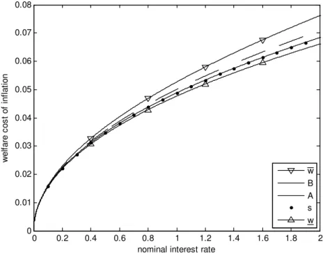
In …gure 1, we plot these …ve measures for the estimated money-demand functionm(r) = 0:05r 0:5_.23

Note howsandA are undistinguishable to the naked eye.

0 0.2 0.4 0.6 0.8 1 1.2 1.4 1.6 1.8 2 0

0.01 0.02 0.03 0.04 0.05 0.06 0.07 0.08

nominal interest rate

welf

are

c

os

t of

inf

lat

ion

w B A s w

Figure 1: Di¤erent measures of the welfare cost of in‡ation for the money-demand speci…cation

m(r) = 0:05r 0:5_.

Another way of …ndingwwould be to …rst ask ourselves what is the'underlying the money-demand handed out to us, and then use (8). Looking at equation (7), we …rst calculate the integral that appears there:

Z m

1

K 1=

1 + K 1=

d =

Z m

1

K1=

1= _+K1= d = Z m

1

d Z m

1

1 ₂

K1= ₊ 1 1d

= logm

1

Z K1= _+m1 1

K1= ₊₁

du u = log

0 @m

,

K1= +m1 1 K1= _{+ 1}

!1 1

A.

Therefore that equation gives us

'(m) = Cm

K1= _+m1 1

, (38)

for a positive constantC. So' =C, and

w(r) = 1 '(m(r))

' = 1

m(r)

K1= _+m(r)1 1

= 1 Kr

K1 K+K1 r 1 1

= 1 1

(Kr1 _{+ 1)}1 ,

which coincides with the previous result.

4.2

The relative measuring di¤erence

and (37), we get

(r) := w(r) w(r)

w(r) =

8 < :

1 + 1+(1 Kr

1 ₎ 1

1 (1+Kr1 ₎ 1 , ifr >0

0, ifr= 0

.

Write f(x) =

8 < :

1 + 1+(1 x) 1

1 (1+x) 1 , ifx >0

0, ifx= 0

, so that f(Kr1 ) = (r). So we obtain (with the

recommended aid of a mathematics software) the following third-order Maclaurin expansion forf:

f(x) = 0 + 1 1 x+

1 2(1 )2x

2₊ 2 2+ 5 5

12(1 )3 x

3_+O(x4_),

where O(x4_{) means a function whose absolute value is less than a constant times x}4_{, for small enough} values ofx(we’re only interested in reasonable interest rates, which correspond to lowx’s).

Now write g(x) = 1 1 + (1 x) 1 _{, wherex 0, as a guess for an approximation tof (insights}

gained by looking at their graphs, see Figure 2). That is, g is de…ned so thatg Kr1 ₌ 1_{w(r). Its} third-order Maclaurin expansion is

g(x) = 0 + 1 1 x+

1 2(1 )2x

2₊ 2

6(1 )3x

3_+O(x4_).

Therefore, for smallx, we havef(x) =g(x) +O(x3_{). Puttingx=Kr}1 _{, this can be rewritten as}

(r) = 1w(r) +O(r3 3 ) (39)

= 1 h 1 + 1 Kr1 1i_+O(r3 3 _),

which is a good approximation to this relative di¤erence formula. Figure 2 gives an even better idea of how good this approximation is.

0 0.5 1

0 0.01 0.02 0.03 0.04 0.05 0.06

rel

at

iv

e

m

eas

uri

ng

di

ff

erenc

e

0 0.5 1

0 0.02 0.04 0.06 0.08 0.1 0.12

nominal interest rate

0 0.5 1

0.25 0.3 0.35 0.4 0.45 0.5 0.55 0.6 0.65 0.7

real difference approximation

Figure 2: The real relative measuring di¤erence and its approximation, 1w, for the speci…cations

m(r) = 0:05r 0:1,m(r) = 0:05r 0:5and m(r) = 0:05r 0:9.

Note that, for practical purposes, we can have an idea of how relevant this di¤erence is by entering

between 2.88% and 3.12% – a very precise con…dence interval. So one can be at ease about which measure to take, when considering low-in‡ation countries. On the other hand, consider a country where the annual in‡ation rate has reached 400% (in Brazil, for instance, in‡ation reached 1783% in 1989). In this case, for the same parameters, the relative measuring di¤erence reaches 22% (considering r = 4, since the long-term real interest rate would become negligible), which is to say that one has to be really careful about which measuring strategy is being used, in the case of hyperin‡ations.

4.3

Formulas for the multidimensional welfare measures

Let’s now extend the log-log money-demand speci…cation to the multidimensional case. It is natural enough to propose an extension of the form

(m_{) =} K G(m₎

1=

rG(m_),

where K > 0 and 2 (0;1). The reader should notice that this is the demand that follows from (38) and (21). It is also worth noticing that, in the usual case where G is a weighted geometric mean,

G(m1; : : : ; mn) = Qn_i=1mii (where i 0, 8i 2 f1; : : : ; ng and Pn

i=1 i = 1), we would obtain the

system of equations ₈

> > > < > > > :

1(m) =

K1= 1

m1

Qn

j=1m

(1 1₎ j

j

.. .

n(m) =

K1=

n

mn

Qn

j=1m

(1 1₎ j

j

,

which, inverted,24 gives a demand in the format

8 > > < > > :

m1(u) =L1Qnj=1u

1j

j

.. .

mn(u) =LnQnj=1u nj

j

,

where ij is the demand elasticity of typeiof money relative to the opportunity cost of holding type j.

Again,B andAare straightforward. Taking as in subsection 3.1, we have:

B(m_{) =}

Z

( ) d = K1=

Z

rG(m_{) d}m G(m₎1= = K

1= G(m)

1 1 1 1 m +1 = K 1=

1 G(m)

1 1

, (40)

and

A(m_{) =}

Z

( ) d

1 + ( ) =

Z

K1= dG(m₎ G(m₎1= _+K1= _G(m).

Notice how this is exactly the same integrand that appeared in our second approach to …nding win the unidimensional case. With that knowledge behind us, we can immediately write:

A(m_{) = lim}

G !+1

2 4

Z G

G(m)

dG~

~

G 1

Z K1= _{+(G )}1 1

K1= _+G(m)1 1

dG~

~

G

3 5

= lim

G !+1log

2 6

4 G

K1= _+G 1 ₁ 1

K1= _+G(m)1 1 1

G(m₎

3 7 5 = log 0 B @

K1= _+G(m)1 1 1

G(m₎

1 C

A= ₁ log 1 +K1= G(m₎1 1 _{. (41)}

2 4_{The very name of this kind of demand gives us a hint of how to invert this system of equations: apply the logarithm}

Here we have made implicit use of the obvious fact that, sinceGis a positive, increasing in each variable and1-homogeneous function, it is unbounded: limm!+1G(m) = +1.

Then (41) and (32) give at once

w(m_{) = 1 1 +K}1= _G(m₎1 1 1 _{. (42)}

Now forw. Equation (29) takes, in this case, the form

wxi(m) = (1 +w(m))

1= K

G(m₎

1=

Gxi(m),

which, as in the unidimensional case, gives

Z w(m) 0

d

(1 + )1= = K

1= Z rG(m) dm

G(m₎1= =B( m_),

so that

1

1 1 (1 +w(m)) 1 1

1 = K

1=

1 G(m)

1 1

,

and

w(m_{) = 1 + 1 K}1= _G(m₎1 1 1_{. (43)}

Finally, for s, the easiest thing to do is just imitate (33) in the obvious way, and verify that it satis…es (17). That is, takesgiven implicitly by equation

D(m_{; s(}m_{)) = 0, (44)}

where

D(m; s) := K

1=

1 G(m)

1 1

+ (1 s) 1 (1 s) 1= .

The Implicit Function Theorem gives

sxi(m) =

@D

@xi (m; s(m))

@D

@s (m; s(m))

=

1_K1= _G(m) 1=

Gxi(m)

1 + 1 1 _{(1 s(m))} 1=

= i(m)

1 + (1 ) 1 (1 s(m₎₎ 1=

,

whence

1

sxi(m)

= 1

i(m)

(1 ) 1 (1 s(m₎₎ 1=

K1= _G(m) 1= _G

xi(m)

.

Substituting from (44), we get

1

sxi(m)

= 1

i(m)

+ K

1= _G(m)1 1

K1= _G(m₎ 1= _Gx

i(m) (1 s(m))

= 1

i(m)

+ G(m)

Gxi(m) (1 s(m))

,

an expression equivalent to (17). The reader may wish to check that these formulas really extend the unidimensional ones.

All these measures are plotted in Figure 3, where n = 2, K = 0:05 and = 0:5. In Figure 3a,G is taken so that G(m; x) = m0:5x0:5, and in Figure 3b, G(m; x) =m0:7x0:3. The ordering of the surfaces is the one implied by Proposition 2. Again, as in the unidimensional case, we see thatAapproximates s

0

0.05

0.1

0.15

0.2

0 0.05 0.1 0.15 0.2

0 0.1 0.2 0.3 0.4

cash bank deposits

welf

are

c

os

t of

inf

lat

ion

Figure 3a: Di¤erent measures of the welfare cost of in‡ation for the money-demand speci…cation₍

m= 0:025r 0:75_{(r r}

x)0:25

x= 0:025r0:25(r rx) 0:75

.

0

0.05

0.1

0.15

0.2

0 0.05 0.1 0.15 0.2

0 0.1 0.2 0.3 0.4

cash bank deposits

welf

are

c

os

t of

inf

lat

ion

Figure 3b: Di¤erent measures of the welfare cost of in‡ation for the money-demand speci…cation₍

m=0:05 0:70:65

0:30:15 r 0:65r0_x:15 x= 0:05 0:30:85

0:70:35 r0:35rx0:85

.

4.4

Obtaining this demand from our models