IBM Research, Brazil biancazbr.ibm.com
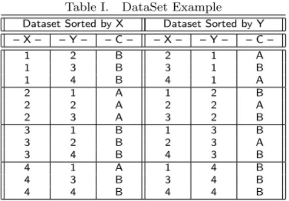
Texto
Imagem
Documentos relacionados
Os princípios constitucionais gerais, embora não integrem o núcleo das decisões políticas que conformam o Estado, são importantes especificações
É importante destacar que as práticas de Gestão do Conhecimento (GC) precisam ser vistas pelos gestores como mecanismos para auxiliá-los a alcançar suas metas
Neste trabalho o objetivo central foi a ampliação e adequação do procedimento e programa computacional baseado no programa comercial MSC.PATRAN, para a geração automática de modelos
No caso e x p líc ito da Biblioteca Central da UFPb, ela já vem seguindo diretrizes para a seleção de periódicos desde 1978,, diretrizes essas que valem para os 7
de maneira inadequada, pode se tornar um eficiente vetor de transmissão de doenças, em especial àquelas transmitidas pela via fecal-oral, capazes de resultar em
Essa característica das línguas do grupo ao qual pertencem o latim e o português torna relevante a investigação da evolução da fonologia para a compreensão da evolução
O número de dealers credenciados para operar com o Banco Central do Brasil é de vinte instituições e estas devem sempre participar de leilões de câmbio quando promovidos pelo
Cuida-se de Comunicado Interno n.º 027/2021 e Decisão da Pregoeira Oficial acostada aos autos do Processo Administrativo n.º 442/2020 da Tomada de Preços n.º 016/2020, cujo objeto
