Braz. J. Phys. vol.33 número1

Interplanetary Shock Parameters during Solar

Activity Maximum (2000) and Minimum (1995-1996)

E. Echer

, W. D. Gonzalez

, L. E. A. Vieira

, A. Dal Lago

,

F. L. Guarnieri

, A. Prestes

, A. L. C. Gonzalez

, and N. J. Schuch

1

Instituto Nacional de Pesquisas Espaciais, INPE - S. Jos´e dos Campos, SP, Brasil

2

Centro Regional Sul de Pesquisas Espaciais, CRSPE/INPE - Santa Maria, RS, Brasil

Received on 22 May, 2002. Revised version received on 5 September, 2002

Interplanetary shock parameters are analyzed for solar maximum (year 2000) and solar minimum (years 1995-1996) activity. Fast forward shocks are the most usual type of shock observed in the interplanetary medium near Earth’s orbit, and they are 88% of the identified shocks in 2000 and 60% in 1995-1996. Average plasma and magnetic field parameters for upstream and downstream sides of the shocks were calculated, and the parameter variations through the shock were determined. Applications of the Rankine-Hugoniot equations were made, obtaining shock speeds and Alfvenic Mach number. Static and dynamic pressures variations through the shocks were also calculated. Every parameter have larger variation through the shock in solar maximum than in solar minimum, with exception of the proton density. The intensity of shocks relative to the interplanetary medium, quantified by the Alfvenic Mach Number, is observed to be similar in solar maximum and minimum. It could be explained because, during solar maximum, in despite of the higher shock speeds, the Alfvenic speed of the interplanetary medium is higher than in solar minimum.

I

Introduction

The interplanetary medium has a very low particle density, of about 5 m

3

, and it has a collisional mean free path of about 1 Astronomical Unit(AU) or1:5:10

8

km[1]. Thus

the occurrence of particle collisions is very sporadic. How-ever, the interplanetary space is transiently disturbed by col-lisionless shock waves. In these shocks, the role that parti-cle collisions make in ordinary shocks, is performed by long range Coulombian forces [1-4]. These Coulombian forces can have this very important role because the interplanetary medium is ceaseless permeated by the solar wind, a plasma resulting of the solar corona expansion and that carries with it the solar magnetic field through the solar system [1,5]

Shock waves detected near the Earth’s orbit, 1 AU, are mainly caused by interplanetary remnants of solar ejecta, although some types of shocks could be generated by in-teraction regions between slow and high speed solar wind streams [5]. Solar ejecta are coronal material expelled from the Sun, the coronal mass ejections [1,6-10] which propa-gate through the interplanetary medium. A shock occurs when the relative speed between a high speed stream and the background solar wind is higher than the characteristic speed of the medium (Alfvenic, magnetossonic)[1,2,3,5].

Interplanetary structures can be geoeffective, causing magnetic storms, especially if an intense and long dura-tion southward component of the magnetic field is present

[6,11,12]. Because shock waves have a larger spatial extent than the interplanetary structures, it is usual that spacecrafts near Earth’s orbit measure only the shock. However, the shock itself can have geoeffective effects, especially sudden impulses - increase in the H component of the geomagnetic field observed in low and mid latitudes stations, due to the intensification of Chapman-Ferraro current in the magne-topause, and magnetohydrodynamics waves and micropul-sations propagation inside Earth’s magnetosphere [1,13].

In this work we are studying interplanetary shock pa-rameters during high and low solar activity conditions. The years of 2000 (solar maximum) and solar minimum (1995-1996) were selected for analysis. Plasma and magnetic field parameter variations through the shocks were calculated, and derived quantities for shocks - shock speed, Alfvenic Mach Number, magnetic field and plasma compression and plasma and magnetic field pressures were calculated in order to evaluate the differences in these shock parameters during solar activity maximum and minimum.

II

Data

space-craft [15] in solar maximum. We have analyzed 15 fast for-ward shocks in 1995-1996 and 50 fast forfor-ward shocks in 2000. For 6 events during 2000, plasma sensor onboard ACE was saturated, and plasma data were obtained from Proton Monitor onboard the SOHO spacecraft [16]. All data were obtained via internet, through the International Solar-Terrestrial Physics Program data services.

III

Results and discussion

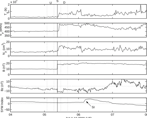
Figure 1 shows an example of a fast forward interplanetary shock on July 10th 2000. From the top to the bottom, panels are: proton temperature Tp (K), speed Vp (km/s) and density Np(m

3

), total magnetic field Bt (nT), north-south mag-netic field component Bz (nT) and the SYM geomagmag-netic index (nT). The shock is indicated by the letter ”S” and by the continuous line. It is observed that plasma parameters

and total magnetic field jump through the shock, creating a discontinuity. Less than one hour after the shock, a sud-den impulse (SI in the Fig. 1) is observed in the SYM index, indicating a H geomagnetic field component increase, corre-sponding to the Earth’s magnetosphere compression by the shock and the intensification of the Chapman-Ferraro cur-rent in the magnetopause.

In order to calculate the plasma and Bt variation through the shock, three time windows were defined, each one of about 10 min. The boundaries of these time windows are limited by the dotted lines in Fig. 1. The central time dow corresponds to the shock itself. The lateral time win-dows correspond to the upstream and downstream sides of shock [5] and are labeled in Fig. 1 by the letters ”U” and ”D” respectively. Average parameters were calculated for the in-terval limited by upstream and downstream time windows, and the difference between these averages is quantified as the parameter variation through the shock.

0 1 2x 10

5

Tp

(k)

350 400 450 500

V p

(km/s)

0 10 20

Np

(cm

3)

0 10 20

B (nT)

−10 0 10

Bz (nT)

04 05 06 07 08

−50 0 50

SYM Index

JULY 10 2000 (UT) S

U D

SI

Figure 1. Example of a fast forward shock observed on 10th July 2000. Panels are proton temperature, speed and density, total magnetic field, north-south magnetic field component and the geomagnetic SYM index. The continuous line indicate the shock and the dashed lines indicates the upstream, shock and downstream time windows (see text).

During solar maximum and minimum a total of 57 and 25 shocks were identified, respectively. This difference oc-curs because during high solar activity, a larger number of solar transients are expelled from the solar corona [6,8,10] than during low solar activity. These shocks were classi-fied analyzing the parameter variations, in forward (fast and slow) and in reverses (fast and slow). The parameter varia-tions through every type of shock are shown in a sketch in Fig. 2.

be-cause solar wind is moving supersonically away from the Sun, both types of shocks are moving away from the Sun, relatively to the Sun itself and any satellite that measures the parameters [5]. A shock is fast when its relative speed

to the solar wind is higher than the fast magnetossonic wave speed; a shock is slow when its relative speed is higher than the slow magnetossonic wave speed.

Time Time

Time

slow reverse shocks fast reverse shocks

Relative variation Relative variation

Relative variation

slow forward shocks

Bt Np

Vp Tp fast forward shocks

Relative variation

Time

Bt Np

Vp Tp

Vp Np Tp

Bt

Tp

Np

Bt

Vp

Figure 2. Sketch of parameter variations: Tp, Np, Vp and Bt, for the four types of interplanetary shocks. Upper left panel,fast forward, right, slow forward shocks. Lower left panel, fast reverse, right, slow reverse shocks.

Fast forward shocks show positive jumps in all the vari-ables, Vp, Tp, Np and Bt. Slow forward shocks show pos-itive jumps in Vp, Tp and Np, but negative in Bt, because slow magnetossonic waves have plasma and magnetic field variations anticorrelated [3]. Reverse shocks present posi-tive jumps in Vp, because solar wind is dragging the shock. For both slow and fast reverse shocks, Np and Tp have neg-ative jumps. For fast reverse shocks, Bt has negneg-ative jumps, whereas for slow reverse shocks Bt has positive jumps (an-ticorrelated to plasma jump).

Figure 3 shows bar graphs expressing the percentage of every type of shock in solar maximum (left) and in solar minimum (right). It is seen in Fig. 3 that the large major-ity of shocks are of the fast forward type, in solar maximum (88% or 50 shocks of 57) and in solar minimum (60% or 15 shocks of 25). This distribution occurs because fast inter-planetary ejecta are the main driver of shocks near Earth’s orbit. It is also observed that in solar maximum the number of fast forward shocks is about ten times higher than in so-lar minimum, 50/year in maximum against 7.5/year in soso-lar minimum; a proportion ten times higher in maximum was expected because coronal mass ejections rate is about ten times higher in solar maximum than in solar minimum [8].

Slow shocks (forward and reverse) occur in smaller numbers, and they are relatively more abundant in solar min-imum than in solar maxmin-imum. Generally slow shocks occur near the stream interface, which are barriers to the flow and contribute to the plasma and magnetic field draping [5].

fast reverse fast forward slow reverse slow forward

0 10 20 30 40 50 60 70 80 90 100

Percentage of shocks

Type of shock

solar maximum solar minimum

Figure 3. Bar graph distribution of types of interplanetary shocks in solar maximum (white bars) and in solar minimum (gray bars).

holes are long duration phenomena, during several solar ro-tations (27 days) and reaching the Earth recursively at peri-ods near a solar rotation [6]. The high speed streams interact with the heliospheric current sheet, which is characterized by slow speed and high density streams, and their interac-tion creates the so-called corrotating interacinterac-tion regions [6], that compress the interplanetary magnetic field, intensifying it. This interaction region is bounded by forward and reverse shocks. However, at 1 AU this CIR is not totally developed, and the so-called proto-CIRS are observed [6].

The reverse shocks observed in this work are probably related to the interaction regions. Fast forward shocks are mainly caused by coronal mass ejections, but it is possible that some fast forward shocks, especially in solar minimum,

are caused by interaction regions.

In the remaining of this paper fast forward shocks are selected to analyze the plasma and magnetic field parame-ter variations through the shock and the differences between solar maximum and solar minimum.

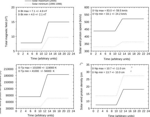
Figure 4 shows the averages of Bt, Vp, Tp and Np, re-spectively, for upstream and downstream sides of shocks. The continuous curve is the step-like variations for solar maximum and the dotted line for solar minimum. The time axis is in arbitrary units. Upstream averages can be consid-ered as representative of the background solar wind condi-tions, whereas downstream average values are representative of the solar wind disturbed by shocks.

0 2 4 6 8 10 12 14 16 18 20 22 24 5

10 15 20

D Bt max = 7.1 +/- 4.9 nT D Bt min = 4.0 +/- 2.1 nT

Time (arbitrary units) Time (arbitrary units)

Solar maximum (2000) Solar minimum (1995-1996)

0 2 4 6 8 10 12 14 16 18 20 22 24 300

350 400 450 500 550 600

D Vp max = 83.0 +/- 59.5 km/s D Vp min = 33.1 +/- 24.2 km/s

Solar wind proton density (cm

-3)

Time (arbitrary units) Time (arbitrary units)

Solar wind proton speed (km/s)

0 2 4 6 8 10 12 14 16 18 20 22 24 30000

60000 90000 120000 150000 180000

210000 D Tp max = 101000 +/- 119000 K D Tp min = 41000 +/- 56000 K

Solar wind proton temperature (K) 0 2 4 6 8 10 12 14 16 18 20 22 24

5 10 15 20 25 30 35

D Np max = 10.7 +/- 11.0 cm -3

D Np min = 13.7 +/- 10.0 cm -3

Total magnetic field (nT)

Figure 4. Step-like parameter variations through interplanetary shocks. Upper left panel, Bt variation and right, Vp variation. Lower left panel, Tp variation and, right Np variation. Continuous lines are for solar maximum and dotted line for solar minimum.

It is seen that upstream and downstream parameter av-erages of Bt, Vp and Tp are larger in solar maximum than in solar minimum, whereas for Np the higher values are ob-served in solar minimum. These averages are similar for the whole period, as seen in Table I, for 1995-1996 and 2000. These results can be explained because in solar minimum, the heliospheric plasma sheet/heliospheric current sheet is more stable, located near low solar latitudes and near to Earth; then the interplanetary medium near Earth has high

values of solar density and low speeds/temperature. In solar maximum, the heliospheric current sheet has a waving varia-tion, and alternatively the interplanetary medium near Earth has periods with high and low density, that causes average density in solar maximum to be lower than in solar mini-mum [17]. Thus interplanetary shocks in solar minimini-mum are propagating in a medium with higher densities than in solar maximum.

Table I Average solar wind parameters for solar maximum and minimum. Parameter Solar minimum 1995-1996 Solar maximum 2000

Vp 425.095:0km/s 455.0110:0km/s

Tp 6100063000K 7600091000K

Np 9.56:1m

3

7.76:3m 3

During solar maximum the Sun is more active, launch-ing more ejecta with higher magnetic field intensity and so-lar wind speed, what could justify the higher values of these parameters in solar maximum [18]. However, plasma and magnetic field parameters show a solar cycle variation su-perimposed with smaller-scale fluctuations and in each so-lar cycle the form of variation seems to be slightly different [18]. Particularly, total magnetic field seems to have a vari-ation in phase with sunspot cycle, but density has an oscilla-tion of around 5 years [20].

Density variation through shocks is slightly higher in so-lar minimum (13.710:0m

3

) than in solar maximum (10.7

11:0m 3

) but the difference is not very large. On the other hand, the proton speed and temperature, and total magnetic field averages are much higher in solar maximum than in so-lar minimum. Especially, the speed variation is on average more than two times higher in solar maximum than in solar minimum (83.059.0 km/s against 3324.2 km;s) as a

consequence of the fact that in solar maximum, solar ejecta and their interplanetary remnants are more intense and with higher speeds [10].

Rankine-Hugoniot equations

Every type of magnetohydrodynamics shocks should ob-serve the Rankine-Hugoniot equations [1,2,3,5], which are fundamental physical relationships for a plane surface of discontinuity (shock), through of it physical fields jump from the upstream to the downstream sides. These equa-tions express the mass, normal momentum flux, tangential momentum flux, energy and magnetic flux conservations. Burlaga [5] presents these equations relative to a reference system with origin at the shock. It is supposed that the upstream and downstream speeds are radials, so the shock speed can be calculated, relative to the Sun, in eq.(1):

U = N 2 V 2 N 1 V 1 N 2 N 1 (1) WhereN 1, N 2, V 1, V

2 are average density and speed

in the upstream and downstream sides, respectively. With eq. (1), the shock speed was calculated. The relative distri-bution (in percentage) of shock speeds are shown in upper panel of Fig. 5 for solar maximum (left) and solar minimum (right). The average shock speeds are higher for solar max-imum than for solar minmax-imum, as expected, with significant differences (594.4192.0 km/s in maximum against 394.0 46.5 km/s in minimum). During solar minimum the

dis-tribution of speeds is more concentrated, between 300-500 km/s, with the majority of shocks occurring between 350-400 km/s (53% of the events). During solar maximum, the distribution of shocks has a large spread, with events with shock speed around or larger than 1000 km/s.

The ratio between the flow speed and the characteris-tic speed of the medium is called the Mach number. For an interplanetary shock, its Mach number will be given in terms of the ratio of the relative speed between shock and the solar wind and the characteristic speed (magnetossonic

or Alfvenic). In this work the Alfvenic Mach number is cal-culated for the shocks studied. The Alfven speed for the solar wind can be calculated using the parameters of the up-stream side in eq. (2):

V A = B 1 ( 0 1 ) 1=2 (2)

In eq. 2,B

1and

1are the total magnetic field and mass

density in the upstream side ( 1 = n 1 m + ) and 0 is the

magnetic permeability. The Alfvenic Mach number can then be calculated by eq. (3):

M A = jU V 1 j V A (3)

where U is the shock speed (equation 1) andV

1 is the

up-stream speed.

In Fig. 5, in the intermediate panels, the Alfvenic Mach Number is shown for solar maximum, at left and for solar minimum, at right. At the solar system, shocks can be found to have until a Mach number of 20 [1]. In the present study it was observed that Alfvenic Mach number of shocks are in the range 2-3, with some extremes until 7-8.

It is seen that the average Mach numbers are very similar in solar minimum and in solar maximum, in despite of shock speeds higher during solar maximum. This result could be explained because the Alfven speed depends on the density and magnetic field of the medium. Proton density is higher in solar minimum than in solar maximum, whereas magnetic field is greater in solar maximum, and the resulting Alfven speed should be lower in solar minimum. Average values for upstream conditions for Alfvenic speed are69:626:2

km/s in solar maximum and34:322:0km/s in solar

min-imum. Thus in solar minimum, the Alfven speeds are on average 2 times lower than in solar maximum, and shocks with lower speeds than shocks in solar maximum will have Alfvenic Mach numbers higher or similar equal to faster shocks at solar maximum. These results show that shock strength, relatively to the solar wind, is similar in both solar activity periods, because the propagation medium is differ-ent and the variation in the Alfvenic speed compensates the shock speeds variation, for the period studied.

Intermediate lower panels in Fig. 5 show the total mag-netic field ratio ((B

2)/( B

1)). The compression ratio

distri-bution and the average values are very similar for both so-lar minimum and maximum. It is also seen that the mag-netic compression ratio is always higher than 1, and lower than 4. The value of 4 for compression is the theoretical fi-nite compression limit in the case of high Mach numbers, for a monoatomic gas [1]. However, for density compres-sion ratio, shown in the last panel in Figure 5, values of compression higher than 4 are seen in about10%of shocks

in solar maximum. The distributions are similar, with av-erage density compression ratio higher in solar maximum (2:601:10) than in solar minimum (2:100:62). During

be because this limit was derived for shocks exactly perpen-dicular [1], and in our dataset is possible to have a distri-bution of shocks between parallel and perpendicular types. Furthermore, the compression ratio of magnetic field and

plasma depends of the way as the shock heats the plasma and individual events could be different of the adiabatic ap-proximation considered in obtaining the expression for the compression ratio [1].

200 400 600 800 1000 1200 1400 1600 0

20 40 60

U = 594.4 +/- 192.0 km/s

Relative Occurrence (%)

Shock speed Us (km/s)

Relative Occurrence (%)

Shock speed Us (km/s)

200 400 600 800 1000 1200 1400 1600 0

20 40 60

U = 394.0 +/- 46.5 km/s

1 2 3 4 5 6 7 8 9 10 0

20 40 60 80 100

M_A = 2.30 +/- 1.44

Alfvenic Mach Number Alfvenic Mach Number

1 2 3 4 5 6 7 8 9 10 0

20 40 60 80 100

M_A = 2.45 +/- 1.92

0 1 2 3 4

0 20 40 60

Density Compression ratio r (N2/N1) Density Compression ratio r (N2/N1)

r = 1.97 +/- 0.57

Magnetic field Compression ratio r (B2/B1) Magnetic field Compression ratio r (B2/B1)

0 1 2 3 4

0 20 40

60 _{r = 1.99 +/- 0.63}

SOLAR MINIMUM (1995-1996) SOLAR MAXIMUM (2000)

0 1 2 3 4 5 6 7 8 0

20 40 60

r = 2.60 +/- 1.10

0 1 2 3 4 5 6 7 8 0

20 40

60 _{r = 2.10 +/- 0.62}

Figure 5. Upper panels, calculated shock speeds for solar maximum (left) and solar minimum (right). Intermediate panels, Alfvenic Mach number in solar maximum (left) and in solar minimum (right). Lower intermediate panels, magnetic field compression ratio in solar maximum (left) and in solar minimum (right). Bottom panels, density compression ratio in solar maximum (left) and in solar minimum (left).

Pressure calculations

In the fluid description of a plasma, the definition of ideal gas pressure can be applied, and the momentum con-servation can be expressed as a pressure balance. The ther-mal pressure of plasma is calculated in eq.(4):

p T

=N

p kT

p

(4)

In eq. (4)N

p and

T

p are the proton density and

tem-perature, and k is the Boltzmann constant. The magnetic pressure is also defined in terms of the total magnetic field, in eq. (5) [1,4].

p B

= B

2

2 0

(5)

The thermal and magnetic pressures are called static pressures of plasma. The momentum flux of plasma is also called dynamic pressure and it is expressed in eq. (6):

p dyn

=N

p m

+ V

2 p

(6)

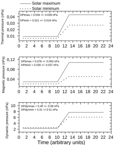
Figure 6 shows the calculation of the thermal, magnetic and dynamic pressures variations through the shocks, as a step-variation between upstream and downstream sides. The

pressures are given in units of nPa and the time is in arbi-trary units. It is seen that pressure values both at upstream and downstream sides are higher in solar maximum than in solar minimum. Also the step-like variations are higher for solar maximum. Another interesting point to observe is that the dynamic pressure is higher by almost 2 magnitude orders than magnetic and thermal pressures. These results indicate that the majority of energy/momentum flux is in kinetic form instead of thermal or magnetic energy. Actually, in the so-lar wind, about 99% of the pressure is in form of dynamic pressure [1].

IV

Conclusions

0 2 4 6 8 10 12 14 16 18 20 22 24

2 4 6 8

10 DPdynmax = 5.40 +/- 5.08 nPa

DPdynmin = 4.31 +/-3.51 nPa

Dynamic pressure (nPa)

Time (arbitrary units)

Solar minimum

0 2 4 6 8 10 12 14 16 18 20 22 24

0,04 0,08

0,12 _{DPbmax = 0.078 +/- 0.093 nPa} DPbmin = 0.030 +/- 0.037 nPa

Magnetic pressure (nPa)

0 2 4 6 8 10 12 14 16 18 20 22 24

0,01 0,02 0,03

0,04 DPtmax = 0.034 +/- 0.039 nPa DPtmin = 0.021 +/- 0.019 nPa

Thermal pressure (nPa)

Figure 6. Upper panel, step-like calculated thermal pressure variations (in nPa) for solar maximum(continuous line) and solar minimum (dotted line). Intermediate and lower panels, magnetic and dynamical pressures variations.

Plasma and magnetic fields parameters have higher upstream-downstream averages and variations in solar max-imum than in solar minmax-imum, with exception of the proton density. Proton density is higher in solar minimum prob-ably because of the heliospheric current sheet, which has a higher density than the background environment, and is more stable during solar minimum conditions. Shock speed variation is much higher in solar maximum (average speed variation of 83 km/s) than in solar minimum (33.1 km/s). The shock speed is also larger in solar maximum (594 km/s against 394 km/s in minimum), because in solar maximum the solar ejecta have higher speeds.

Alfvenic Mach number and magnetic field compression ratio are very similar for both solar maximum and solar min-imum. Shocks strength, quantified by Mach Alfvenic num-ber, is similar in solar maximum and solar minimum, be-cause higher shock speeds in solar maximum are being com-pensated by higher Alfvenic speeds.

Thermal, magnetic and dynamic pressure variations through the shocks are larger in solar maximum than in so-lar minimum, as expected because the majority of parame-ters have a stronger variation in solar maximum. Moreover, it was observed that dynamic pressure values are about two orders of magnitude higher than thermal and magnetic pres-sure, which confirms that a large fraction of solar wind en-ergy is in form of kinetic enen-ergy.

Acknowledgements

The authors would like to acknowledge the Brazilian agencies FAPESP, CAPES, and CNPq.

References

[1] M. G. Kivelson and C. T. Russell, Introduction to Space

Physics, Cambridge University Press, New York(1995).

[2] R. G. Stone and B. T. Tsurutani, Collisionless shocks in the

heliosphere: A tutorial review, Geophysical Monograph 34,

American Geophysical Union, Washington DC (1985).

[3] R. Z. Sagdeev and C. F. Kennel, Scientific American, April, 40 (1991).

[4] G. K. Parks, Physics of Space Plasmas, an introduction, Addison-Wesley Publishing Company, Redwood City, CA (1991).

[5] L. F. Burlaga, Interplanetary Magnetohydrodynamics, Ox-ford University Press, New York (1995).

[6] W. D. Gonzalez, B. T. Tsurutani, and A. L. Cla de Gonzalez, Space Science Reviews 88, 529 (1999).

[7] J. T. Gosling, D. J. McComas, J. L. Phillips, and S. J. Bame, Journal of Geophysical Research 96, 7831 (1991).

[9] R. Schwenn, Space Science Reviews 44, 139 (1986).

[10] R. Schwenn, Advances in Space Research 26, 43 (2000).

[11] J. W. Dungey, Physics Reviews Letters 6, 47 (1961).

[12] W. D. Gonzalez and B. T. Tsurutani, Planetary Space Science

35, 1101 (1987).

[13] E. J. Smith, J. A. Slavin, R. D. Zwickl, and S. J. Bame Solar Wind Magnetosphere Coupling, Terra Scientific Publishing Company, Tokyo, 345 (1986).

[14] M. H. Acu˜na, K. W. Ogilvie, D. N. Baker, S. A. Curtis, D. H. Fairfield, and M. H. Mish, Space Science Reviews 71, 5 (1995).

[15] E. C. Stone, A. M. Frandsen, R. A. Mewaldt, E. R.

Chris-tian, D. Margolies, J. F. Ormes, and F. Snow, Space Science Reviews 86, 1 (1998).

[16] V. Domingo, B. Fleck, and A. I. Poland, Space Science Re-views 70, 7 (1994).

[17] E. Whipple and H. Lancaster, Space Science Reviews 71, 41 (1995).

[18] P. R. Gazis, Reviews of Geophysics 34, 379 (1996).

[19] D. F. Webb and R. A. Howard, Journal of Geophysical Re-search 99, 4201, (1994).