Dark Energy and the Accelerated
Expansion of the Universe
Ioav Waga
Universidade Federal do Rio de Janeiro, Instituto de Fsica Rio de Janeiro, RJ, 21945-970, Brazil
E-mail: [email protected] Received 7 January, 2000
Recent observations indicate that the expansion of the Universe is accelerating. This suggests the existence of some kind of exotic matter with negative pressure. The simplest possibility is a cosmological constant but there are alternatives, as for instance an evolving scalar eld. In this paper we explore constraints from lensing statistics and high-z type Ia Supernovae on some of these alternatives.
I Introduction
\I am a detective in search of a criminal { the cosmicalconstant. I know he exists, but I do not know his appearance; for instance I do not know if he is a little man or a tall man. Naturally the rst move of my chief (de Sitter) was to order a search for footprints, or what look like footprints::: :::I think I have now about enough evidence to justify an arrest." Arthur Eddington in\The Expanding Universe".
Recent observations of type Ia supernovae (SneIa) suggest that the expansion of the Universe is accelerat-ing [1, 3]. In fact what it is observed is that high-z SneIa { that after corrections are almost perfect standard can-dles { are fainter than would be expected in a Universe where the expansion is slowing down or remain con-stant. Although there are still some possible sources of systematic eects (source evolution and dust are those that concern most), the current accepted explanation is that they appear fainter because in a Universe that is speeding up distances are larger. To get a qualitative understanding of why accelerated expansion leads to larger distances consider a nearby source with measured redshift z. Forget for a while peculiar velocities and think on redshift as a simple Doppler eect. In this ap-proximation, for nearby sources the measured redshift can be thought as giving us the velocity of the pho-ton source at the time it was emitted(z=ve=c). Now consider the velocity-distance law [4]: v(t) =H(t)d(t), where v is the value of the source velocity and d its proper distance at the same timet. Let us consider t the present time. So, if in the past the photon source had Hubble ow velocity ve and the rate of the
Uni-verse expansion is speeding up, the present value of the source velocity is larger now than it would be in case the Universe expands with, for instance, constant velocity. So, assuming the same value for the Hubble parameter today, it follows from the velocity-distance law, that a larger velocity implies a larger distance. It follows from Friedman equation (a=a=;(4 G=3)(+ 3p)) that ac-celerated expansion may be achieved if the Universe has a dominant component with an eective negative pres-sure. Dark energy, dynamical- (dynamical vacuum energy) or quintessence are dierent names that have been used to denote this component. A cosmological constant is its simplest form.
Recent studies incorporating new CMB data [5, 6] conrm previous analysis suggesting a large value for the total density parameter (total > 0:4) and favor a nearly at Universe. Further, a dierent set of ob-servations [7] now unambiguously indicate low values (m0 = 0
:30:1) for the matter density parameter (m0). In combination these two results are in line with the conventional interpretation of the SneIa re-sults and all together strongly support at cosmolo-gies with m0
0:3 and a dark energy component with X 0:7. These models are also theoretically appealing since a smooth component on small scales (20{30h
;1
Mpc) reconcile ination with the low values for m0[8].
show how the age of the Universe could be greater than the inverse value of the Hubble parameter accepted at that time. The cosmological term was also kept dif-ferent from zero by Eddington [11], who preferred the cosmological expansion starting from an Einstein static universe. Petrosian, Salpeter and Szekeres [12] intro-duced this term to account for an apparently observed preponderance of sources with redshift z'2, and Gunn and Tinsley [13] invoked it in 1975 to explain a seem-ingly accelerated expansion of the universe. For a re-view on the early history of the cosmological constant see North [14]. Several aspects of non null cosmolo-gies such as the age problem, classication of models, classical tests, observational constraints on , struc-ture formation and gravitational lenses were discussed by several authors. For a review and/or an extensive list of references see [20].
In the past the cosmologicalconstant has been intro-duced several times to reconciliate theory with observa-tions. When better data became available or improved interpretation showed it was not needed, has always been discarded. However, now it is possible that this situation will change and that the \genie" will remain, perhaps for ever, out of the bottle [19]. According to quantum eld theory, the vacuum state has zero-point uctuations to whose energy the gravitational eld is sensitive. As is well known, Lorentz invariance implies that the vacuum contribution to the energy-momentum tensor must be of the form g , where g is the met-ric tensor. Therefore, quantum eld theory predicts a cosmological term that added to the bare cosmological constant gives rise to an eective cosmological term. The problem then lies in the maximum value that ob-servations indicate to this term,
<
3mpl2H2 0 8 ; or
< 10
;56cm;2:
The above upper limit is 50 to 120 orders of magnitude below the estimate given by quantum eld theory. The diculty in explaining the smallness of the eective is known as the \cosmological constant problem". One of the original motivations for introducing the idea of a dynamical -term was to alleviate this problem. There are also observational motivations. For instance, in these models the COBE normalized amplitude of the mass power spectrum is in general lower than in the conventional constant- model, in accordance with ob-servations [24]. Further, the distance to an object with redshift z is smaller than the distance to the same ob-ject in a constant- model (assuming the same value
of m0). So, constraints coming from lensing statistics are weaker in these models [15, 18].
The dynamical- models present in the literature can schematically be divided in three types: scalar eld [31, 23, 24, 26, 25], x-uid [29, 30, 18] and decaying-laws [28, 17, 16]. A phenomenological decaying- law model in which decreases as /a
;m [here a is the scale factor of the Friedman-Robertson-Walker (FRW) metric and m is a constant (0m < 3)] was suggested in Refs.[17, 16]. It was observed that the Einstein equations for these models are the same if instead of a -term, it would be considered (beside matter and radia-tion) a x-uid with equation of state, px=;
m
3 ;1
x.
In spite of the similarity at the level of Einstein equa-tions, these two phenomenological models are dierent. For instance, in the case of a decaying -term, matter is created as a result of the decaying vacuum, while in the exotic uid description the x-component is conserved.
In this paper we shall deal with two cosmologi-cal tests: gravitational lensing statistics and the SneIa magnitude redshift test. As mentioned before the strongest observational support for an accelerated uni-verse comes from SneIa. This test can be considered the main motivation for introducing some kind of ex-otic matter with negative pressure. On the other hand, most lensing statistics analysis give lower values for and we nd interesting to compare the predictions of these two important tests. Here we rst consider the special case where the exotic component is a x-uid with constant equation of state and that is smooth on scales smaller than horizon. We also report constraints from gravitational lensing statistics and high-z SneIa on two representative scalar eld potentials that give rise to eective decaying models: PNGB potentials (V () = M4(1 + cos(=f))) and inverse power-law po-tentials (V () = M4+;). There are dierent moti-vations for introducing these two potentials. The best motivation for the PNGB potential comes from particle physics while the inverse power-law potentials have the property of \tracking" that allow the eld to start with a wide set of initial conditions [32].
Let us consider rst the motivations for introducing the PNGB potential[21, 23, 25]. In order to act approx-imately like a cosmological constant at recent epochs with 1, the potential energy density should be of order the critical density, M4
3H
2 0m
2
Pl=8, or
M ' 310
motion of the eld is still (nearly) overdamped, that is, p
jV 00(
0) j
<
3H
0= 5 10
;33h eV. The two conditions above imply that f mPl ' 10
19 GeV. Further, the PNGB mass is mM
2=f '10
;32h eV. In quantum eld theory, such ultra-low-mass scalars are not generi-callynatural: radiative corrections generate large mass renormalizations at each order of perturbation theory. To incorporate ultra-light scalars into particle physics, their small masses should be at least `technically' nat-ural, that is, protected by symmetries, such that when the small masses are set to zero, they cannot be gener-ated in any order of perturbation theory, owing to the restrictive symmetry.
From the viewpoint of quantum eld theory, pseudo-Nambu-Goldstone bosons (PNGBs) are the simplest way to have naturally ultra{low mass, spin{0 particles. PNGB models are characterized by two mass scales, a spontaneous symmetry breaking scale f (at which the eective Lagrangian still retains the symmetry) and an explicit breaking scale M (at which the eective Lagrangian contains the explicit symmetry breaking term). Thus, the two dynamical conditions on f and M above essentially x these two mass scales. Note that
M 10
;3 eV is close to the neutrino mass scale for the MSW solution to the solar neutrino problem, and f mPl ' 10
19 GeV, the Planck scale. Since these scales have a plausible origin in particle physics mod-els, we may have an explanation for the `coincidence' that the vacuum energy is dynamically important at the present epoch [23, 21, 22]. Moreover, the small mass m is technically natural.
Next consider the inverse power-law case. The best motivation for introducing this potential is the existence of attractor (tracking) solutions such that if B, the following relationship is satised: TR a
3( B
; TR
)
B with TR = B =(2 + ) < B
[27, 15, 32]. Here a is the scale factor of the FRW met-ric and B stands for the adiabatic index of the
back-ground (B = 4=3 during the radiation dominated era
and B= 1 during the matter dominated era (MDE)).
So, if the eld is on track its energy density decreases slower than the background energy density and the eld eventually will begin to dominate the dynamics of the expansion. If the eld is on track during the MDE, its eective adiabatic index will be less than unity and the eld eective pressure will be negative. This condi-tion by itself does not guaranty accelerated expansion. It is necessary that the eld dominates the dynamics and that the total eective adiabatic index be smaller than 2/3. However, for inverse power-law potentials at late times ! 1, such that when the growing
starts to become non negligible, deviates from
the above tracking value decreasing toward the value !0. So, even if > 4 such that initially TR > 2=3 in the MDE, as the eld dominates and decreases,
the Universe will enter in a phase of accelerated ex-pansion. If m0 and are suciently low this will happen before the present time. For inverse power-law potentials the two conditions 0
1 and the pre-ponderance of the eld potential energy over its kinetic energy (p
jV 00(
0) j
<
3H
0) imply M
10
27;12
+4 eV
and 0
mPl. Since 0
mPl quantum gravitational corrections corrections to the potential are important and could invalidate this picture [33].
In the very early Universe, in order to success-fully achieve tracking the eld energy density must be smaller than the radiation energy density. If in addition it is smaller than the initial value of the tracking energy density it will remain frozen until they have compara-ble magnitude and then the eld starts to follow the tracking solution. Otherwise, if it is larger than the initial value of the tracking energy density, it will en-ter in a phase of kinetic energy domination ( 2), decreases fast ( / a
;6) overshooting the tracker solution. After that, as in the previous case, the eld frozen and again when the tracking energy density and have comparable magnitude the eld begins to follow
the tracking solution. Whatever is the case there is al-ways a phase before tracking in which the eld is frozen. So, an important point is the value of the eld energy density when it freezes. For instance, is it smaller or larger than eq, the energy density at radiation and
nonrelativistic matter equality? Did the eld had time to completely achieve tracking or not? In fact the con-straints imposed by cosmologicaltests on the parameter space depend on this condition.
We report constraints from lensing statistics and high-z Sne for the inverse power-law potential starting from two dierent set of initial conditions. In the rst one we assume that the eld is frozen by the matter{ radiation equality epoch. This is the approach we fol-lowed in Ref. [25]. In this case depending on the value of and m0, it may happen that the eld does not have time to reach the tracking solution. In general, if m0 is large we observe that is still growing by the present time, away from its initial value = 0.
Otherwise, if m0 is suciently low, will reach a maximum value (not necessarily its tracking value) in the past and , by the present time, will be decreasing to the nal attractor value = 0. In our second
ap-proach we assume that the eld starts tracking very early in the Universe evolution.1 When
becomes
1In fact this is true only if
non-negligible, starts to decrease to its nal
attrac-tor value = 0. Recently constraints from high-z Sne
on power-law potentials with the eld rolling with this set of initial conditions were obtained by Podariu and Ratra[34]. We complement their analysis including the lensing constraints as well.
This paper is based on Refs.[23, 25, 18, 46] and is organized as follows. In Sec.II we present our statis-tical lensing approach. The methods used to obtain constraints from SneIa observations is briey described in Sec.III. In Sec.IV our main results are presented and in Sec.V conclusions are stressed out.
II Lensing statistics
In this section we outline our statistical lensing ap-proach. It is based on Refs:[39, 40] and is described with some more detail in [18]. We start dening the following likelihood function, [39]
Llens=
NU Y
i=1 (1;p
0
i)N
L Y
j=1 p0
j N
L Y
k=1 p0
ck: (1)
Here NL is the number of quasars that have multiple
image, NU is the number of quasars that don't have,
p0
i 1 is the probability that quasar i is lensed and p0
ck is the conguration probability, that we shall
con-sider as the probability that quasar k is lensed with the observed image separation. To perform the statistical analysis we use data from the HST Snapshot survey (498 high luminous quasars (HLQ), the Crampton sur-vey (43 HLQ), the Yee sursur-vey (37 HLQ), the ESO/Liege survey (61 HLQ), The HST GO observations (17 HLQ), the CFA survey (102 HLQ) , and the NOT survey (104 HLQ) [35]. We considered a total of 862 (z > 1) high luminous optical quasars plus 5 lenses.
The dierential probability, d, that a line of sight intersects a galaxy at redshift zL in the interval dzL
from a population with number density nG is,
d = c nGa2
crdt ; (2)
where acris the maximumdistance of the lens from the
optical axes for which multiple images are possible. It is a function of the angular diameter distance between observer and lens, lens and source, observer and source and it also depends on the lens model.
In our approach we use a singular isothermal sphere (SIS) as the lens model, we neglect lensing by spiral galaxies, assume conserved comoving number density of early tipe galaxies, ne= n0(1 + z)
3 and a Schechter
form for the galaxy population, n0=
Z 1 0
n
L L
exp
; L L
dL
L; (3) with n = 0:61 h
310;2Mpc
;3 and =
;1:0. We as-sume that the luminosity satises the Faber-Jackson relation [37], L=L = (
jj= jj)
, with = 4 and take
jj= 225 Km/s.
The total optical depth (), obtained by integrating d along the line of sight from 0 to zS, can be expressed
analytically, (zS) = F30;
dA(0;zS)(1 + zS) 3
(cH;1 0 )
;3; (4) where F = 163n
e(cH;1 0 )
3( jj=c)
4;(1 + + 4=) ' 0:026 measures the eectiveness of the lens in produc-ing multiple images [36].
It is important to include two corrections to the op-tical depth: magnication bias and selection function due to nite resolution and dynamic range [39].
Since lensing increase the apparent brightness of a quasar and since there are more faint quasars than bright ones, there will be over representation of lensed quasars in a ux limited sample. The bias factor is given by [38, 39, 40]
B(m;z) = M 2 0
B(m;z;M
0;M2) ; (5) where
B(m;z;M
1;M2) = 2
dNq
dm
;1 Z M
2
M1 dM M3
dNq
dm (m + 2:5logM;z): (6) Since we are modeling the lens by a SIS prole, M0= 2, and we use M2= 10
4in the numerical computation. We use the following expression for the quasar lu-minosity function [40]
dNq
dm /
10;a(m;m)+ 10;b(m;m)
;1
; (7)
where m =
8 < :
m0+ (z + 1) for z < 1; m0 for 1 < z < 3; m0
;0:7(z;3) for z > 3;
(8) and we assume a = 1:07, b = 0:27 and m0= 18:92. The magnication corrected probabilities are
shown that the selection function corrected probabili-ties are: [39]
p0
i(m;z) = pi
R
dpc()B(m;z;Mf();M 2) B(m;z;M
0;M2)
; (10) and
p0
ci= pci()
pi
p0
i
B(m;z;Mf();M 2) B(m;z;M
0;M2) ; (11) where
pc() = F(zS)
Z z S 0
(1 + zL)3
dA(0;zL)dA(zL;zS)
cH0 ;1d
A(0;zS)
2 8 ? jj c 2 ; 1 cH;1 0 cdt dzL =2 ;( + 1 + 4
)
0 B @
dA(0;zS)
dA(zL;zS)8 ? jj c 2 1 C A 2
(+1+ 4 ) exp 2 6 6 4 ; 0 B @
dA(0;zS)
dA(zL;zS)8
? jj c 2 1 C A 2 3 7 7 5 1 dzL;
(12) Mf() = M0
1 + f
f;1; f > 1 ;
(13) and
f = f() = 100:4m(): (14) To simplify computation we use two selection functions [39], one for the HST observations and another one for all the ground based surveys. Using more accurate se-lection functions for each ground based observations separately have little statistical eect.
Recently Falco et al. [41] observed that statisti-cal lensing analysis based on optistatisti-cal and radio observa-tions can be reconciled if the existence of dust in E/SO galaxies is considered. In our computation we assume a mean extinction of m =0:5 mag as suggested by their estimates. Current statistical analysis using both HLQ and radio sources tight the constraints on a cos-mological constant. Although this combined analysis for dynamical- models is still in progress we can have an idea of what should be expected if, for instance, we reduce extinction in our analysis to m =0:3 mag. In this case the new 2 contours, shift by approximately 1 from the previous one, that is, the new 2 contours will be located slightly before the 1 contours of the gures in Sec.4.
By expressingLlensas a function of the parameters m and m0we obtained the maximum of the likelihood function (Lmaxlens) and formed the ratio l =Llens=Lmaxlens. It can be shown that with two parameters, the distri-bution of ;2lnl tends to a
2 distribution with two degrees of freedom [39].
III High-redshift type Ia
Super-novae [18]
There are two major ongoing programs to systemat-ically search and study high-z supernovae. Although the very preliminary results indicated a low value for the cosmological constant ( < 0:51 at the 95% con-dence level) [43], more recent analysis with larger sam-ple of supernovae, now points to a dierent direction. Now the data indicate an accelerated expansion such that
0:7, m 0
0:3 and strongly supports a at Universe.[1, 2].
In our analysis we consider data from the High-z Supernovae Search Team. We use the 27 low-z and 10 high-z SneIa (we include SN97ck) reported in Riess et al. [1] and consider data with the MLCS [44, 1] method applied to the supernovae light curves. Following a pro-cedure similar to that described in Riesset al.[1], for each model,we determine the cosmological parameters ^a through a 2 minimization neglecting the unphys-ical region m0 < 0. To simplify computation we x the Hubble parameter to H0 = 65:2 km/s Mpc
;1 [1], but the results are independent of this choice for H0[1]. We use
2
sne(^a) =
37 X
i=1
p(zi; ^a); 0;i 2 2 0;i+ 2
vi ; (15)
where
p= 5logdL+ 25; (16)
is the distance modulus predicted by each model, 0is the observed (after corrections) distance modulus, 0 its uncertainty and v is the dispersion in galaxy
red-shift due to peculiar velocities. Following [1] we use vi= 5
ln10
200km=s
czi and for high-z SneIa with z not de-rived from emission lines in the host galaxy, we add 2500 km/s in quadrature to 200 km/s (see Table 1 in [1]).
IV Results [18,46]
Ya. B. Zeldovich We rst consider the x-uid model. In Fig.1 we present contours of constant likelihood 95.4% (2) and 68% (1) arising from the 2
sneanalysis together with
those from lensing (dashed lines). For SneIa the peak of the likelihood is located at m'1:1 and m
0 = 0. If we x m = 0 we get m0= 0:25
0:08 (1). For lensing the maximum of the likelihood occurs for m'2:4 and m0= 0. The same approach when applied to constant models (since m = 0 we now have only one degree of freedom) gives:
<
0:76 (or m 0
>
0:24) at 2, 1> m
0
>
0:39 at 1 with a best t at m 0
'0:61. From the gure it is clear that there is a region in the parameter space (the region inside the triangle with ver-tices (m'0:85,m
0
'0:24), (m = 0,m 0
'0:32) and (m = 0,m0
'0:38)) such that all points are inside the 1 (68%) condence region of both tests.
0 0.25 0.5 0.75 1 1.25 1.5 1.75
m
0 0.1 0.2 0.3 0.4
Ω m
95.4
95.4
68.
68.
68.
95.4
px=[
m 3-1]ρx
Figure 1. Contours of constant likelihood (95:4% and 68%) arising from lensing statistics (dashed lines) and type Ia su-pernovae are shown for the x-uid model.
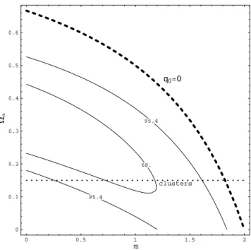
In Fig. 2 we display contours (95:4% and 68%) of the combined (lensing plus SneIa) likelihood. For the combined 2 analysis we used 2
tot = 2
sne;2lnl, with l =Llens=Lmaxlens as dened in Sec.2. Although the peak of the likelihood for each test separately occurs at m0= 0, the maximum of the combined likelihood oc-curs at m = 0 (cosmological constant) and m0
'0:33. Note that best t models of the combined likelihood are in accelerated expansion (q0< 0). Models with m = 2 (cosmic strings [29]) and any value of m0 are at more than 99% c.l. away from the peak of the likelihood. We observe that if, for instance, we take h = 0:65 and Bh2 = 0:02, the CMBR rst acoustic peak (`
p eak),
models with m and m0inside the 1 allowed region in Fig 2, will have `p eakvalues between
'215 and 230, (see Fig. 4 in Ref.[30]), that are close to the current best val-ues for `p eak obtained from CMBR data. Models with parameters m and m0 in this region are in agreement with the current CMBR data as well. Constraints from observations of clusters suggest m0> 0:15 [7]. In Fig. 2 we display this constrain as a dotted line. Models above this line are preferred.
0 0.5 1 1.5 2
m
0 0.1 0.2 0.3 0.4 0.5 0.6
Ω m
95.4
95.4
68.
q0=0
clusters
Figure 2. Contours of combined likelihood (95:4% and 68%) arising from lensing statistics and type Ia supernovae are shown for the x-uid model.
Now we consider the scalar eld models. In Fig.3 we show the 95:4% and 68:3% C. L. limits from lens-ing (short dashed contours) and the SNe Ia data on the parameters f and M of the PNGB potential. As in [25], these limits apply to models with the initial con-dition4
p
(ti)
mPl = 1:5 and
ddt(ti) = 0, with ti = 10;5t 0; for other choices, the bounding contours would shift by small amounts in the f;M plane. We also plot some contours of constant m0(dashed) and the curve q0= 0 (long dashed contour) as a function of the parameters f and M. The best t region of the parameter space is limited by the lensing and SneIa 95:4% C. L. contours and also by m0> 0:15, that we took as our lower limit for m0. The lensing 2 contour roughly coincides with the density parameter contour m0
also favor the region in the parameter space where the eld is still nearly frozen, that is, the region between the almost vertical lines of the 2 lensing and SneIa contours.
0.00225 0.0025 0.00275 0.003 0.00325 0.0035 0.00375 0.004 M [h1/2
eV] 2
3 4 5 6
f
/
10
18
GeV
95.4
95.4
68.3
68.3 95.4 68.3
Ω=0.5
Ω=0.3 Ω=0.15 q0=0
Figure 3. Contours of constant likelihood (95:4% and 68%) arising from lensing statistics (short dashed lines) and type Ia supernovae are shown for the PNGB model.
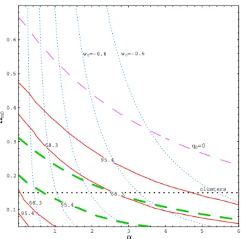
In Figs.4 and 5 we show the 95:4% and 68:3% C. L. limits from lensing (thick dashed contours) and the SNeIa data on the parameters and m0 of the in-verse power-law potential. For Fig.4 we assume that the eld is frozen around the matter{radiation equality epoch, while for Fig.5 the eld starts tracking early in the Universe evolution. Again we display in the gures, as an horizontal straight line, m0 = 0:15 that we took as our lower limit for m0. We also plot some con-tours with the present value of the equation of state w0 = 0
;1 (thin dashed contours) and the curve q0 = 0 (long dashed contour). The present data ex-clude > 5 for the two initial data set we used. We also have w0
<
;0:5 that is also roughly what we got in the x-uid case, that sometimes is used as an ap-proximation for the inverse power-law potential. We also observe that the lensing constraints on the equa-tion of state are weak, constraining only low values of m0and . Although weak they are consistent with the SneIa constraints. We can tight the constraints on the equation of state if we consider a higher value for the m0 lower bound. For instance, if we take m0 = 0:3 as our lower bound (as suggested by large-scale galaxy ows [45]) we obtain w0
<
;0:6 (or
<
4) for the rst initial data set and w0
<
;0:67 (or
<
1:8) for the second one. In both models, a larger lower bound on
m0, pushes the scalar eld behavior toward that of a conventional cosmological constant.
1 2 3 4 5 6
α 0.1
0.2 0.3 0.4 0.5 0.6
Ωm0
95.4
95.4
68.3
68.3
w0=−0.6
w0=−0.7
−0.8 −0.9
q0=0
95.4 68.3
clusters
Figure 4. Contours of constant likelihood (95:4% and 68%) arising from lensing statistics (thick dashed contours) and type Ia supernovae are shown for the inverse power-law model. Also shown is the lower bound m0 = 0
:15 from clusters and curves of constant present equation of state w0=p0=
0. For the gure it is assumed that the eld is frozen at the matter{radiation equality epoch
So far we have considered only at models. For the sake of completeness we also obtained constraints on m0 and in case we relax the atness hypoth-esis and assume a conventional constant . In Fig.6 we show the 95:4% and 68% C. L. limits from lens-ing (short dashed contours) and the SNeIa data on the parameters m0 and . In our lensing analysis we used m = 0:6 mag for extinction. The lines q0 = 0 (dashed) and k = 0 (doted) are also displayed in Fig.6. The long dashed lines are roughly the 2 constraints from CMB anisotropy [6]. The pink shaded area is the best tting region of the parameters. It is quite clear that current data favors an accelerated expansion (right of the q0= 0 line) and a nearly at Universe. This re-gion would be reduced even more if, for instance, we had considered other constraints on m, as those
1 2 3 4 5 6 α
0.1 0.2 0.3 0.4 0.5 0.6
Ωm0
95.4
95.4 68.3
68.3
q0=0
clusters
w0=−0.5
w0=−0.6
95.4
68.3
Figure 5. Contours of constant likelihood (95:4% and 68%) arising from lensing statistics (thick dashed contours) and type Ia supernovae are shown for the inverse power-law model. Also shown is the lower bound m0 = 0
:15 from clusters and curves of constant present equation of state w
0 = p
0 =
0 . For the gure it is assumed that the eld starts tracking early in the Universe evolution.
0 0.5 1 1.5 2
Ω Λ
0 0.5 1 1.5 2
Ω m
q0=0 68
95.4 68
Lensing
CMB
SneIa
k=0
Physically not permited region
q0=0 68
95.4 68
Lensing
CMB
SneIa
k=0
q0=0 68
95.4 68
Lensing
CMB
SneIa
k=0
Physically not permited region
Figure 6. Contours of constant likelihood (95:4% and 68%) arising from lensing statistics (thick dashed contours) and type Ia supernovae are shown for open, at and closed mod-els with constant . The lines q0 = 0 (dashed) and k= 0 (doted) are also displayed.
V Summary
A consensus is beginning to emerge that we live in a nearly at, low-matter-density Universe with m0
0:3 and a dark energy, negative-pressure component with X 0:7. The nature of this dark energy com-ponent is still not well understood; further develop-ments will require deeper understanding of fundamen-tal physics as well as improved observational tests to measure the equation of state at recent epochs, w(t), and determine if it is distinguishable from that of the cosmological constant.
In this paper we considered observational con-straints from lensing statistics and high-z SneIa on cos-mological models whose matter content is nonrelativis-tic matter plus a negative-pressure dark energy compo-nent. We used a lensing approach, where extinction is considered, and that takes into account magnication bias and the selection function due to nite resolution and dynamic range in the conguration probability. For the SneIa analysis we considered data from the High-z Supernovae Search Team, the 27 low-z and 10 high-z SneIa reported in Ref. [1]. We used data with the MLCS method applied to the supernovae light curves. We showed that the two tests are compatible and ob-served that best t models are in accelerated expansion (q
0 <0).
Acknowledgments
This is paper is based on work done with Josh Frie-man and Ana Paula Miceli. I would like to deeply thank them. It is a pleasure to thank Luca Amendola and Franco Occhionero for several useful conversations and discussions during my visit to Rome last year. I would also like to thank Bharat Ratra and Silviu Po-dariu for sending their paper with SneIa constraints on inverse power-law models before publication and for kindly clarifying my understanding on several points. Many thanks to Cindy Ng for discussions and for her interest in our work. This work was supported by the Brazilian agencies CNPq and FAPERJ.
References
[1] A. G. Riess et al.,Astron. J. 116, 1009 (1998). P. M. Garnavichetal., Ap. J.509, 74 (1998).
[2] S. Perlmutteretal., B.A.A.S.,29, 1351 (1997). [3] S. Perlmutteretal., Ap. J.517, 565 (1999). [4] E. Harrison, Ap. J.,403, 28 (1993).
[7] N. A. Bahcall, J. P. Ostriker, S. Perlmutter and P. J. Steinhardt Science, 284, 1481 (1999). M. S. Turner, astro-ph/9901109.
[8] P.J.E. Peebles, Astrophys. J. 284, 439 (1984); M. S. Turner, G.Steigman, L. M. Krauss, Phys. Rev. Lett.52, 2090 (1984).
[9] A. Einstein, Sitzungsberichte der Preussischen Akad. d. Wiss.1917, 142 (1917).
[10] G. Lema^tre, Mon. Not. R. astr. Soc.90, 490 (1931). [11] A. S. Eddington, Mon. Not. R. astr. Soc. 90, 668
(1930).
[12] V. Petrosian, E. Salpeter and P. Szekeres, Ap. J.147, 1222 (1967).
[13] J. R. Gunn, M. B. Tinsley, Nature257, 454 (1975). [14] J. D. North, The Measure of the Universe, Oxford:
Clarendon Press (1965).
[15] B. Ratra and A. Quillen, Mon. Not. R. Astron. Soc., 259, 738, (1992); A. R. Cooray, A&A,342, 353 (1999). [16] L. F. Bloomeld Torres and I. Waga, Mon. Not. R.
Astron. Soc.279, 712 (1996).
[17] V. Silveira and I. Waga, Phys. Rev. D50, 4890 (1994); V. Silveira and I. Waga, Phys. Rev.D56, 4625 (1997) [18] I. Waga and A. P. M. R. Miceli, Phys. Rev. D, 59,
103507 (1999).
[19] Y. B. Zeldovich, Sov. Phys. Uspekhi,11, 381 (1968). [20] W.H. McCrea, Proc. Roy. Soc. London A 206, 562
(1951).; V. Petrosian, in Confrontation of Cosmologi-cal Theories with Observational Data, ed. M. S. Lon-gair (Dordrecht: Reidel), 31 (1974).; B. M. Tinsley, Physics Today, June, 32 (1977).; J. E. Felten and R. Isaacman, Rev. Mod. Phys. 58, 689 (1986).;P. J. E. Peebles, Publ. Astron. Soc. Pac. 100, 670 (1988).; S. Weinberg, Rev. Mod. Phys.61, 1 (1989); L. Abbot, Sci. Am. 258(5), 427 (1989).; S. M. Carrolll, W. H. Press and E. L. Turner, Annu. Rev. Astron. Astrophys.,30, 499 (1992).; For a recent review see V. Sahni and A. Starobinsky, astro-ph/9904398.
[21] J. Frieman, C. Hill, and R. Watkins, Phys. Rev. D46, 1226 (1992).
[22] M. Fukugita and T. Yanagida, preprint YITP/K-1098 (1995).
[23] J. A. Frieman, C. T. Hill, A. Stebbins and I. Waga, Phys. Rev. Lett.75, 2077 (1995).
[24] K. Coble, S. Dodelson, and J. A. Frieman, Phys. Rev. D55, 1851 (1997).
[25] J. A. Frieman and I. Waga, Phys. Rev. D 57, 4642 (1998).
[26] R. R. Caldwell, R. Dave, and P.J. Steinhardt, Phys. Rev. Lett.80, 1582 (1998).
[27] B. Ratra and P. J. E. Peebles, Phys. Rev. D37, 3407 (1988); P. J. E. Peebles and B. Ratra, Ap.J.325, L17 (1988).
[28] M. Ozer and M. O. Taha, Nucl. Phys. B 287, 776 (1987); K. Freeseetal., Nucl. Phys. B287, 797 (1987); M. Reuter and C. Wetterich, Phys. Lett. B188, 38
(1987); W. Chen and Y. S. Wu, Phys. Rev. , 695 (1990); J. C. Carvalho, J. A. S. Lima and I. Waga, Phys. Rev. D46, 2404, (1992); I. Waga, Ap. J. 414, 436; (1993); J. M. Overduin and F. I. Cooperstock, Phys. Rev.D58, 043506, (1998).
[29] A. Vilenkin, Phys. Rev. Lett., 53, 1016 (1984); J. N. Fry, Phys. Lett.B158, 211 (1985); H. A. Feldman and A. E. Evrard, Int. J. Mod. Phys. D 2, 113 (1993); J. Stelmach and M. P. Dabrowski, Nucl. Phys. B406, 471 (1993); H. Martel, Ap. J.445, 537 (1995); L. M. A. Bit-tencourt, P. Laguna, R. A. Matzner, hep-ph/9612350; M. Kamionkowski and N. Toumbas, Phys. Rev. Lett., 77, 587 (1997); D. N. Spergel and U. L. Pen, Ap. J. 491, L67 (1997); M. S. Turner and M. White, Phys. Rev.D56, R4439 (1997);W. Hu, Ap. J.506, 495 (1998); S. Perlmutter, M.S. Turner and M. White, Phys. Rev. Lett.83, 670 (1999); M. Bucher and D. Spergel Phys. Rev.D60, 043505, (1999); L. Wang, R. R. Caldwell, J. P. Ostriker and P. J. Steinhardt, astro-ph/9901388. [30] M. White, Ap. J.506, 485 (1998).
[31] C. Wetterich, Nuclear Physics B,302, 668 (1988); V. Sahni, H. A. Feldman and A. Stebbins, Ap. J. 385, 1 (1992); P. T. P. Viana and A. R. Liddle, Phys. Rev. D 57, 674 (1998); P. Ferreira and M. Joyce, Phys. Rev. Lett.,79, 4740 (1997); Phys. Rev. D58, 023503 (1998); A. Liddle and R. Scherrer, Phys. Rev. D 59, 023509 (1999); J. Uzan, Phys. Rev. D 59, 123510 (1999); P. Binetruy, Phys. Rev D 60, 063502 (1999); A. Masiero, M. Pietroni and F. Rosati, hep-ph/9905346; L. Amen-dola, astro-ph/9908023; astro-ph/9908023; A. Albrecht and C. Skordis, astro-ph/9908085; V. Sahni and L. Wang , astro-ph/9910097;
[32] I. Zlatev, L. Wang and P. J. Steinhardt, Phys. Rev. Lett.,82, 896 (1999); P. J. Steinhardt, L. Wang and I. Zlatev, Phys. Rev D59, 123504 (1999).
[33] S. M. Carroll, Phys. Rev. Lett, 81, 3067 (1998); C. Kolda and D. H. Lyth, Phys. Rev. Lett B 458, 197 (1999); K. Choi, hep-ph/9912218.
[34] S. Podariu and B. Ratra, astro-ph/9910527.
[35] D. Maozetal., Ap. J.409, 28 (1993); D. Crampton, R. D. McClure, and J. M. Fletcher, Ap. J.392, 23 (1992); H. K. C. Yee , A. V. Filipenko, and D. H. Tang, A. J. 105, 7 (1993); J. Surdejetal.ibid.105, 2064 (1993); E. E. Falco, inGravitationalLensesintheUniverse, edited by J. Surdej, D. Fraipont-Caro, E. Gosset, S. Refsdal, and M. Remy (Liege: Univ. Liege), 127 (1994); C. S. Kochanek, E. E. Falco, and R. Shild, Ap. J. 452, 109 (1995); A. O. Jaunsen etal., A&A300, 323 (1995). [36] E. L. Turner, J. P. Ostriker, J. R. Gott III, Ap. J.284,
1 (1984).
[37] S. M. Faber and R. E. Jackson, Ap. J.204, 668 (1976). [38] E. L. Turner, Ap. J.365, L43 (1990); M. Fukugita and E. L. Turner, Monthly Notices Roy. Astron. Soc. 253, 99 (1991).
[39] C. S. Kochanek, Ap. J.419, 12 (1993). [40] C. S. Kochanek, Ap. J.466, 47 (1996).
[42] R. O. Marzke, M. J. Geller, J. P. Huchra and H. G. Corvin, AJ.108, 437 (1994).
[43] S. Perlmutter etal., Ap. J.483, 565 (1997).
[44] A. G. Riess, W. H. Press and R. P. Kirchner, Ap. J. 473, 88 (1996).
[45] I. Zehavi and A. Dekel, Nature , 252 (1999). [46] I. Waga and J. A. Frieman, submitted to Phys. Rev. D