ABSTRACT: The present paper investigates the high-order spectral inite volume method with emphasis on applicability aspects for compressible lows. The intent is to improve the understanding and implementation of numerical techniques related to high-order unstructured grid schemes. In that regard, a hierarchical moment limiter and high-order mesh capability are developed for a 2-dimensional Euler spectral inite volume solver. The limiter formulation and geometry interpreter for high-order mesh generation are new contributions for the spectral inite volume method. Literature test cases are evaluated to assess the interaction of curved mesh, limiter and spatial reconstruction features of the spectral inite volume scheme. An order-of-accuracy study is presented along with steady and unsteady problems with strong shock waves and other discontinuities typical of compressible lows. Moreover, second, third and fourth-order spatial resolution analyses are explored and the spectral inite volume results are compared with those from different numerical methods.
KEYWORDS: Spectral volume method, Compressible lows, High-order reconstruction, Unstructured grids.
Further Development and Application of
High-Order Spectral Volume Methods for
Compressible Flows
Carlos Breviglieri1,João Luiz F Azevedo2
INTRODUCTION
High-order numerical schemes represent the natural extension of current Computational Fluid Dynamics (CFD) methods, which were developed over the past 30 years for aerospace simulations. he current generation methods are mostly 2nd-order accurate in space and have achieved a level of maturity and robustness desirable for everyday use in aeronautical engineering scenarios. Likewise, several complementary methods were developed for time integration, convergence acceleration, shock capturing and geometry lexibility. However, there are many problems that cannot be fully simulated using low-order methods, such as vortex dominated lows. his observation has motivated the CFD community to consider high-order methods for unstructured meshes. Application of discretization orders larger than 2nd-order has been an area of ongoing research for the last decades (Abgrall 1994; Barth and Frederickson 1990; Ollivier-Gooch 1997; Wang et al. 2013). he present paper is aligned with such efort.
The spectral finite volume (SFV) scheme, as proposed by Wang and co-workers (Liu et al. 2006; Sun et al. 2006; Wang 2002; Wang and Liu 2002, 2004; Wang et al. 2004), shares the functionality of a inite volume solver, copes with unstructured meshes and is an eicient alternative to other classes of 2-dimensional (2-D) high-order methods, for instance, the essentially non-oscillatory (ENO) and weighted ENO (WENO) families of schemes (Wolf and Azevedo 2006, 2007). The CFD solution resolution, or quality, is directly related to
1.Departamento de Ciência e Tecnologia Aeroespacial – Instituto Tecnológico de Aeronáutica – Divisão de Ciências da Computação – São José dos Campos/SP – Brazil. 2.Departamento de Ciência e Tecnologia Aeroespacial – Instituto de Aeronáutica e Espaço – Divisão de Aerodinâmica – São José dos Campos/SP – Brazil. Author for correspondence: João Luiz F Azevedo | Departamento de Ciência e Tecnologia Aeroespacial | Instituto de Aeronáutica e Espaço – Divisão de Aerodinâmica | Praça Marechal Eduardo Gomes, 50 – Vila das Acácias | CEP: 12.228-904 – São José dos Campos/SP – Brazil | E-mail: [email protected]
the spatial discretization and numerical methods involved. he geometric discretization typically consists of a pre-processing step in which a mesh is generated around the object of interest. Such mesh must be loaded in memory during computation to provide data on model geometry and domain boundaries.
he present study uses a 2-D, inite volume, unstructured CFD solver as a starting point for the development of a high-order method (Breviglieri et al. 2010a). he primary objective is to use the SFV numerical method to solve compressible lows at various speed regimes. he SFV method in 2-D allows one to assess the diiculties and advantages of high-order reconstruction in representative test cases, with proper discontinuity and boundary treatment techniques, in a manageable framework. Such techniques are, in principle, extendable to other high-order methods and also for 3-dimensional (3-D) problems.
Two complementary techniques for the high-order method are explored here, namely, the high-order boundary representation and limited reconstruction. In order to keep the high-order method competitive with the lower-order ones, a high-order representation of the geometric boundaries is necessary to reduce the total number of mesh cells. Such high-order boundary representation improves the numerical resolution and convergence aspects of the method, as indicated in Wang and Liu (2006). he use of limiters is necessary when the low solution contains discontinuities, in order to remove spurious oscillations that may eventually lead to divergence of the numerical solution. Previous study on limiter implementations for high-order methods (Breviglieri et al. 2010b, 2008) was based on problem-dependent parameters to ind out which cells need limiting, which can limit too many or too few elements of the solution. In the irst case, the order of the method is seriously reduced and, in the second one, divergence can occur. To circumvent this drawback, the study here discussed uses a parameter-free generalized moment limiter (Yang and Wang 2009) based reconstruction to deal with discontinuities. he new limiter does not require input constants from the user, rendering the code more robust.
The numerical solver is implemented for the solution of the 2-D Euler equations in a cell-centered inite volume context for triangular meshes. he reported indings and tools are relevant for the long-term goal of numerical analysis over complex 3-D conigurations. he study is also motivated by the authors’ institute mission, which is to design and build satellite launchers and probes. As a consequence, the research addresses high Mach number lows in the context of high-order schemes.
GOVERNING EQUATIONS
he 2-D Euler equations are solved in their integral form as:
(1)
(2)
(4)
(5)
(6)
where P →= EÎ + Fĵ. he application of the divergence theorem to Eq. 1 yields:
he vector of conserved variables, Q, and the convective lux vectors, E and F, are given by:
he standard CFD nomenclature is being used here. Hence, ρ is the density, u and v are the Cartesian velocity components in the x and y directions, respectively, p is the pressure, and et is the total energy per unit volume. he system is closed by the equation of state for a perfect gas:
where the ratio of speciic heats, γ, is set as 1.4 for all computations in this study. In the inite volume context, for stationary meshes, Eq. 2 can be rewritten for the i-th mesh cell as:
where Qi is the cell averaged value of Q at time t; Vi is the volume, or area in 2-D, of the i
-
th mesh element; Si is the surface that surrounds the Vi volume.NUMERICAL FORMULATION
SPATIAL DISCRETIZATION
In order to solve Eq. 5, a k-th-order approximation of the integral is computed. The computational domain, Ω, is discretized into N non-overlapping triangles such that:
hese triangles are referred to as the spectral volumes (SVs).
he solution process involves the deinition of proper initial and boundary conditions to the computational domain.
For a given order of spatial accuracy, k, using the SFV method, each SVi cell must be further divided in sub-cells or control
volumes (CVs). where (xrq, yrq) and wrq are, respectively, the Gaussian quadrature point coordinates and the weights on the r-th edge of CVi,j; nq = integer[(k + 1) / 2] is the number of quadrature points required on the r-th edge for k-th order accuracy.
Due to the discontinuity of the reconstructed values of the conserved variables over SV boundaries, one must use a numerical lux function to approximate the lux values along the spectral volume boundaries. his means that →f (q(xrq, yrq)), which appears in Eq. 12, must come from an appropriate numerical lux if the r-th edge of CVi,j is also an external edge of SVi. Moreover, at any moment during the simulation, one can compute the SV-averaged conserved variable vector, Qi, for the i-th spectral volume, as:
(7)
(8)
(9)
(10)
(11)
where d is the physical dimension of the problem of interest. If one denotes by CVi,j the jth control volume of SVi, the cell-averaged conserved variables, q, for CVi,j at time t are computed as:
where Vi,jis the volume of CVi,j.
Once the CV cell-averaged conserved variables are available for all CVs within SVi, a polynomial pi (x, y)∈Pk-1 of degree k − 1
can be reconstructed to approximate each component of q as:
where h represents the maximum edge length of all CVs within SVi. The polynomial reconstruction process is discussed in detail in the following section. For now, it is sufficient to say that this high-order reconstruction is used to update the cell-averaged state variables at the next time step for all the CVs within the computational domain. Note that this polynomial approximation is valid within SVi and the use of numerical fluxes are necessary across SV boundaries.
Integrating Eq. 5 in CVi,j, one can obtain the integral form for the CV mean state variable:
where →f = EÎ + Fĵ at the CV level; Ar represents the length of the r-th edge of CVi,j; nf is the number of edges of CVi,j. he boundary integral in Eq. (10) can be further discretized into the convective operator form:
he integration on the right side of Eq. 11 can be performed numerically with a k-th order accurate Gaussian quadrature formula as:
(12)
(13)
he calculation of the SV-averaged values is important at the end of the computation in order to analyze the high-order numerical solution at the original grid level. he average is also used to recover the conserved variable vectors for the SVs, which are required for the limited reconstruction process as discussed in the section “Limited Reconstruction”.
he lux integration across CV boundaries that lie on the SV edges involves 2 discontinuous states, to the let and to the right of the edge. A numerical lux is used to solve for this discontinuous state. Note that the normal lux component needs to be continuous in order to maintain conservation. In the present study, the Roe lux diference splitting method (Roe 1981) with entropy ix is used to compute the numerical lux. As the method is based on one of the forms of a Riemann solver, it introduces the upwind efects and, hence, the artiicial dissipation terms into the SFV method.
he semi-discrete SFV scheme for updating the values of conserved properties for the CVs can be written as:
(14)
the equivalent convective operator, C(qi,j), for the j-th control volume of SVi. he numerical lux can be expressed as:
as discussed in Wolf and Azevedo (2006), where the n and n + 1 superscripts denote, respectively, the values of the properties at the beginning and at the end of the n-th time step. he α coeicients are α1 = 3/4, α2 = 1/4, α3 = 1/3, and α4 = 2/3. he C operator represents the discretized convective operator as indicated in Eq. 14.
GENERAL FORMULATION FOR HIGH-ORDER RECONSTRUCTION
he evaluation of the conserved variables at the quadrature points is necessary in order to perform the lux integration over the mesh cell faces or mesh cell edges, in the 2-D case. hese evaluations can be achieved by reconstructing conserved variables in terms of some base functions using the degrees-of-freedom (DOFs) within a SV. he present paper has carried out such reconstructions using polynomial base functions. Hence, let P k − 1 denote the space of (k − 1)-th
degree polynomials in 2 dimensions. hen, the minimum dimension of the approximation space that allows P k − 1 to be
complete is deined by Eq. 7. In order to reconstruct q in P k − 1,
it is necessary to partition the SV into Nk non-overlapping CVs, such that:
(15)
(16)
(17)
(18)
(19)
(20)
(21)
(22)
Here, B is the Roe matrix (Roe 1981) in the edge-normal direction, which has 4 real eigenvalues, namely, λ1 = vn – a, λ2 = λ3 = vn , λ4 = vn + a where vn is the velocity component normal to the edge and a is the speed of sound. Let T be the matrix composed of the right eigenvectors of B. hen, this matrix can be diagonalized as:
where Λ is the diagonal matrix composed of the eigenvalues of B, which can be written as:
Hence, the |B| matrix is formed as:
where Λ and T are calculated as a function of the Roe averaged properties (Roe 1981). Furthermore, |Λ| is formed with the magnitude of the eigenvalues.
It is important to emphasize that some edges of the CVs, resulting from the partition of the SVs, lie inside the original SV in the region where the polynomial is continuous. For such edges, there is no need to compute numerical luxes, as previously described. Instead, one uses analytical formulas for the lux computation and, hence, no artiicial dissipation is required for such edges and the lux computation is extremely fast.
TEMPORAL DISCRETIZATION
In order to advance Eq. 14 in time, an explicit, multi-stage, Runge-Kutta time-stepping method is considered, unless otherwise stated. In particular, the 3-stage total variation diminishing (TVD) Runge-Kutta scheme is used, i.e.,
The reconstruction problem, for a given continuous function in SViand a suitable partition, can be stated as inding pk − 1
∈
P k − 1 such that:With a complete polynomial basis, el(x, y)
∈
P k − 1, itis possible to satisfy Eq. 21. Hence, pk − 1 can be expressed as:
where e is the basis function vector, [e1, …, eNk]; b is the reconstruction coeicient vector, [b1, …, bNk]T. It should be
Figure 1. Triangular spectral volume partitions for (a) linear, (b) quadratic and (c) cubic reconstructions.
Figure 2. Quadratic (a) and cubic (b) isoparametric SV elements.
If q – denotes the [qi,1, …, qi,Nk]T column vector, Eq. 23 can
be rewritten in matrix form as:
HIGH-ORDER BOUNDARY REPRESENTATION From the formulation described so far, it is clear that any input mesh will be divided into a iner mesh and, in principle, render the computation more costly. In the standard 2nd-order inite volume scheme, the mesh boundaries are represented as line segments. his coarse approximation of the geometry results in a cluster of mesh nodes into highly-curved boundaries simply to represent the curved nature of it, for instance, in regions such as the leading edge of an airfoil.
If such approach is carried over to the SFV method, there is no gain in computational performance. he solution is to use high-order geometric elements in the mesh, efectively curving the edges of cells along the domain boundaries. For the present study, quadratic and cubic boundary representations are addressed, respectively, for the 3rd- and 4th-order SFV schemes and only for the elements located at wall boundaries.
In order to perform this representation, one can adopt isoparametric SV cells and map them to the boundary data. However, this particular SV will difer in the partition design from the other SVs. hus, it will require a dedicated recons- truction and shape function values for property interpolations.
For a quadratic SV, one needs to specify 6 nodes, while, for a cubic SV, 10 nodes, as shown in Fig. 2. In order to perform the transformation, one can use the following relation to map a particular triangle of the mesh to the standard element, partition it there, and map it back to the physical domain to get the new nodes of the CV faces,
(23)
(24)
(26)
(27) (25)
where the S reconstruction matrix is given by
Hence, the reconstruction coeicients, b, can be obtained as:
provided that S is non-singular. Substituting Eq. 26 into Eq. 22, pk − 1 is, then, expressed in terms of shape functions, L = [L1, …, LNk], deined as L = eS−1, such that one could write:
Equation 27 gives the value of the conserved state variable, q(x, y), at any point within the SV and its boundaries, including the quadrature points. Note that q – in the equation takes the form as a column vector, as presented in Eq. 24. The previous equation can be interpreted as an interpolation of a property at a point using a set of cell averaged values and the respective weights, which are set equal to the corresponding cardinal base value evaluated at that point.
Once the polynomial base functions, el, are chosen, the L shape functions are uniquely defined by the partition of the spectral volume. The shape and partition of the SV can be arbitrary, as long as the S matrix is non-singular. A detailed discussion of quality and stability analysis of the SFV method partitions can be found in Breviglieri et al. (2008). The partitions used in the present paper follow the orientations given in van den Abeele and Lacor (2007) and they are shown in Fig. 1.
(a) (b) (c)
1 1
4
4
2 2
5
5
3 3
6
6 7 8
9 10
Figure 4. Mid-face nodes, in red, for quadratic boundary reconstruction computed from actual geometry deinition.
where →r = (x, y) and Mj are the shape functions for the transformation.
Once the “curved” SV is partitioned, the interpolation shape functions and the CV edge normals must be recalculated. Note that, typically, only 1 edge of the SV stands at a boundary, as depicted in Fig. 3.
(28)
The interpolation could render wrong values if one of the neighbors is close to a sharp corner or if mirrored meshes are used, with the same x-coordinates for some mesh nodes.
A solution to this problem was to implement a geometry interpreter inside the solver. Within every simulation, the user provides the geometry prescribed by splines in the IGES format (Gruttke 1995). No matter how complicated the geometric construct is for a particular coniguration, the present approach always obtains the correct node correspondence, as illustrated in Fig. 4.
Figure 3. Simpliied quadratic (a) and cubic (b) SVs with one curved boundary edge.
1
4
2 3
1 4
2 5 3
herefore, one could use a simpliied formulation for this speciic edge. In such case, the mapping becomes
for the quadratic SV, and
(29)
(31)
(32)
(33) (30)
for the cubic SV. he simpliied formulation is utilized throughout this study.
One particular challenge is to precisely obtain the mid-face node at the curved edge. he authors previously tried to work with neighborhood interpolation to determine its position, but such approach is not generally applied to “diicult” geometries.
he surface integral in the physical domain, Eq. 12, is also transformed to a surface integral for the standard element in the computational domain. Let the equation of the r-th face of Ci,j in the standard SV be
hen, along this face,
Since η = ηr (ξ) is a line segment in the standard element, η´ r is a constant, evaluated as (η2 – η1)/ (ξ2 – ξ1). Furthermore, along such a face,
(a) (b)
out and mark “troubled cells” which are, in the 2nd stage, limited.
For the detection and limiting process, the limiter employs a Taylor series expansion for the reconstruction (van Altena 1999) with regard to the cell-averaged derivatives. he troubled cells are, then, limited in a hierarchical manner, i.e., from the highest-order derivative to the lowest-order one. If the highest derivative is not limited, the original polynomial is preserved and so is the order of the method at the element level.
his limiter technique is capable of suppressing spurious oscillations near solution discontinuities without loss of accuracy at local extrema in smooth regions. Originally, this limiter methodology was developed for the spectral diference method in Yang and Wang (2009). In the present study, the formulation is extended for the SFV method. he extension here reported applies some ideas from previous research on ENO and WENO schemes (Wolf and Azevedo 2006) in the calculation of the limited properties. It should be emphasized that there are other approaches which implement a similar hierarchical moment limiter formulation for the SFV scheme (Xu et al. 2009), but with slight diferences, in comparison to the present approach, on the calculation of the derivatives for the limited reconstruction.
Several markers (or sensors) were developed and employed for unstructured meshes over the past decades. For an in-depth review, the interested reader is referred to Qiu and Shu (2006). he limiter marker used in the present paper is termed Accuracy-Preserving TVD (AP-TVD) marker (Yang and Wang 2009). One important aspect is that the troubled-cell and limited properties are inherent to the SV element, and not to the CVs in which the lux calculations are performed. Once the SV element is conirmed as a troubled cell, its polynomial, based on CV cell-averaged variables, can no longer be used in any lux integration point, because the property function is no longer smooth within such SV. Hence, it is of utmost importance to limit as few SVs as possible.
To that end, the marker is designed to irst check for the lux integration points in each SV and mark those that do not satisfy the monotonicity criterion. However, if an extremum is smooth, the irst derivative of the solution, at such point, should be locally monotonic. Hence, in a second moment, and using derivative information, as described in the forthcoming discussion, the limiter sensor unmarks those SVs that have smooth local extrema and were unnecessarily marked as troubled cells. herefore, for instance, for a quadratic reconstruction, the limiting process can be summarized in the following stages: he face unit normal vector, n → = (nx, ny), is deined as:
Hence, it is recomputed for the curved faces. It easily follows from Eq. 28, for instance, that
for the simplified quadratic SV. Analogous formulation is applied for the y derivatives and, also, for the simpliied cubic SV. he surface integral, then, becomes
his line integral in the standard element can be evaluated using the standard Gauss quadrature formulation:
where wq represents the Gauss quadrature weights; fRoe is the numerical lux function.
he numerical integration, then, follows the discussion presented in section “Spatial Discretization”.
LIMITED RECONSTRUCTION
For the Euler equations, in the presence of low discontinuities, it is necessary to limit reconstructed properties at lux integration points to produce a converged simulation. The present limiter technique involves 2 stages. First, the solver must ind (34)
(35)
(36)
(37)
1. For a given spectral volume, SVi, compute the minimum and maximum cell averages using a local stencil which
includes its immediate face neighbors, i.e., where r → is the centroid coordinate vector. • A scalar limiter for this face is computed according to
2. he i-th cell is considered as a possible troubled cell if
where (xrq, yrq) identii es a quadrature point in the outer edges of SVi. Note that pi here denotes the reconstruction polynomial of order k − 1 of the i-thSV cell, in the sense of Eq. 22. h e 1.001 and 0.999 constants are not problem-dependent. h ey are simply used to overcome machine error, when comparing 2 real numbers, and to avoid the trivial case of when the solution is constant in the neighborhood of the spectral volume considered. h is step is performed in order to check the monotonicity criterion over the SV cells for which a troubled reconstruction might exist. 3. Since the previous steps may l ag more SVs than strictly
necessary, the next operations attempt to unmark SVs in smooth regions of the l ow. Hence, for a given marked spectral volume, a minmod TVD function is applied to verify whether the cell-averaged 2nd derivative is bounded by an estimate of the 2nd derivative obtained using cell-averaged 1st derivatives of the neighboring spectral volumes. Such test is performed as:
• If the unit vector in the direction connecting the centroids of the i-th and nb-th cells is denoted →l = lxi ˆ + ly j ˆ, where nb indicates the face-neighbor of a marked SVi, the 2nd derivative in such direction is dei ned as:
(39)
(40) or
(41)
(42) • In a similar fashion, the i rst derivatives in the same
l →
direction, for both i-th and nb-thcells, can be computed as:
• Another estimate of the secondderivative, in the →l direction, can be obtained as:
(43)
(44)
(45)
(46)
(47)
(48) • h e process is repeated for the other faces of SVi,
and the scalar limiter for the SV is the minimum among those computed for the faces, i.e.,
• If ϕ(2)i = 1, the second derivatives are bounded, as
previously dei ned, and, hence, SViis actually in a smooth region of the l ow. h erefore, SVi is unmarked. 4. If the previous test is not satisi ed, this means that
the particular SVi spectral volume should indeed be limited. In this case, the limiter for the i rst derivative reconstruction must also be computed. h e calculation procedure follows the same approach as for the second derivatives, and it can be summarized as:
• An estimate of the i rst derivative in the →l direction is calculated as:
• Such estimate is compared to the cell-average i rst deriva-tive in the →l direction, computed according to Eq. 42, in order to obtain the scalar limiter for the face as:
• As before, the scalar limiter for the cell is the minimum of those limiters computed for the faces, i.e.,
RESULTS
The results presented here attempt to validate the implementation of the data structure, temporal integration, numerical convergence stability and resolution of the SFV method. The overall performance of the method is compared with that of a 2nd-order monotonic upstream-centered scheme for conservation laws (MUSCL) scheme and a 3rd-order WENO scheme implementations. The latter uses an oscillation indicator proposed by Jiang and Shu (1996), with the modification of Friedrich (1998). The Roe numerical flux is also used with both schemes. Moreover, the geometric coefficients for the WENO reconstructions are computed in a pre-processing step and kept in memory during the computation. For more details on the MUSCL and WENO scheme formulations, the interested reader is referred to the study in Barth and Jespersen (1989) as well as Wolf and Azevedo (2006, 2007).
For the results here reported, density is made dimensionless with respect to the freestream condition, and pressure is made dimensionless with respect to the freestream density times the freestream speed of sound squared. All numerical simulations are carried out on a 16-core 3.2 GHz PC Intel64 architecture, with Linux OS. The code is written in Fortran 95 language, and the Intel Fortran Compiler® with optimization flags is used. For the performance comparisons, which are presented in this section, all residuals are normalized by the firstiteration residue.
SCALAR CONSERVATION LAWS
h e accuracy of the SFV method is tested for the linear scalar advection equation:
(50)
(49)
h e matrix terms are the SV area moments and they can be computed, up to the desired order of accuracy, by numerical integration as:
The SV area moments are computed during an initial stage of the numerical solver and kept in memory for efficiency. The nb1 to nb5 subscripts represent the neighbors of SVi that form the computational stencil to compute the averaged derivatives. This stencil is determined by an ENO-based search, as in Wolf and Azevedo (2006), for the smoothest SV set. Since only a small number of SVs is selected for limited reconstruction, the overhead of this search does not adversely affect the overall performance of the scheme.
It is also important to observe that, considering all the information already available in a SFV method implementation, there are other possible approaches to compute the averaged derivatives. Actually, such approaches can be more computationally ei cient than the one here adopted. h e interested reader is referred, for instance, to the study presented in Yang and Wang (2009) for further details of one of such alternative approaches. Finally, the quadratic limited polynomial, which is used in order to obtain property values at the quadrature points for a troubled SVi spectral volume, is given by:
(51)
h e area moments terms, M… in the previous equation, are computed as in Eq. 50 by replacing the m and n exponents with the appropriate order. h e limited reconstruction is based on primitive variables {ρ, u, v, p}T, instead of conserved variables,
as one can readily check for non-physical values as, for instance, negative pressures (Bigarella and Azevedo 2007, 2012). Once these properties are available from the limited reconstruction, the vector of conserved variables is easily obtained to resume the numerical l ux integration.
(52) the appropriate order. h e limited reconstruction is based on
, instead of conserved variables, as one can readily check for non-physical values as, for instance,
with a Δt value of 10−4, in order to make the discretization error
time-step independent. Furthermore, the hierarchical limiter is considered in this test to verify if its marker formulation is able to ignore smooth solutions.
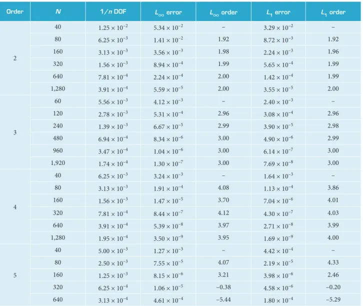
Table 1 shows the L1and L∞ error norms produced using the SFV method with equidistant CVs for t = 1. One can observe that the 2nd-, 3rd- and 4th-order schemes are capable of achieving the expected order of accuracy even on coarse grids. However, the performance of the 5th-order method is not as good.
his behavior is related to the oscillatory pattern of the polynomial interpolation, due to the equidistant distribution, as previously observed by Wang and Liu (2004). As the grid is reined, the errors actually increase in both norms, which give negative orders of accuracy.
Table 1. Accuracy assessment of the 1-D SFV method for the linear scalar advection equation. Equidistant CV partition.
Order N 1/n DOF L
∞
error L∞
order L1 error L1 order2
40 1.25 × 10⁻² 5.34 × 10⁻² – 3.29 × 10⁻² –
80 6.25 × 10⁻³ 1.41 × 10⁻² 1.92 8.72 × 10⁻³ 1.92
160 3.13 × 10⁻³ 3.56 × 10⁻³ 1.98 2.24 × 10⁻³ 1.96
320 1.56 × 10⁻³ 8.94 × 10⁻⁴ 1.99 5.65 × 10⁻⁴ 1.99
640 7.81 × 10⁻⁴ 2.24 × 10⁻⁴ 2.00 1.42 × 10⁻⁴ 1.99
1,280 3.91 × 10⁻⁴ 5.59 × 10⁻⁵ 2.00 3.55 × 10⁻⁵ 2.00
3
60 5.56 × 10⁻³ 4.12 × 10⁻³ – 2.40 × 10⁻³ –
120 2.78 × 10⁻³ 5.31 × 10⁻⁴ 2.96 3.08 × 10⁻⁴ 2.96
240 1.39 × 10⁻³ 6.67 × 10⁻⁵ 2.99 3.90 × 10⁻⁵ 2.98
480 6.94 × 10⁻⁴ 8.34 × 10⁻⁶ 3.00 4.90 × 10⁻⁶ 2.99
960 3.47 × 10⁻⁴ 1.04 × 10⁻⁶ 3.00 6.14 × 10⁻⁷ 3.00
1,920 1.74 × 10⁻⁴ 1.30 × 10⁻⁷ 3.00 7.69 × 10⁻⁸ 3.00
4
40 6.25 × 10⁻³ 3.24 × 10⁻³ – 1.64 × 10⁻³ –
80 3.13 × 10⁻³ 1.91 × 10⁻⁴ 4.08 1.13 × 10⁻⁴ 3.86
160 1.56 × 10⁻³ 1.47 × 10⁻⁵ 3.70 7.04 × 10⁻⁶ 4.01
320 7.81 × 10⁻⁴ 8.44 × 10⁻⁷ 4.12 4.30 × 10⁻⁷ 4.03
640 3.91 × 10⁻⁴ 5.39 × 10⁻⁸ 3.97 2.71 × 10⁻⁸ 3.99
1,280 1.95 × 10⁻⁴ 3.50 × 10⁻⁹ 3.95 1.69 × 10⁻⁹ 4.00
5
40 5.00 × 10⁻³ 1.27 × 10⁻³ – 4.42 × 10⁻⁴ –
80 2.50 × 10⁻³ 7.55 × 10⁻⁵ 4.07 2.19 × 10⁻⁵ 4.33
160 1.25 × 10⁻³ 8.15 × 10⁻⁶ 3.21 3.98 × 10⁻⁶ 2.46
320 6.25 × 10⁻⁴ 1.06 × 10⁻⁵ –0.38 4.58 × 10⁻⁶ –0.20
640 3.13 × 10⁻⁴ 4.61 × 10⁻⁴ –5.44 1.80 × 10⁻⁴ –5.29
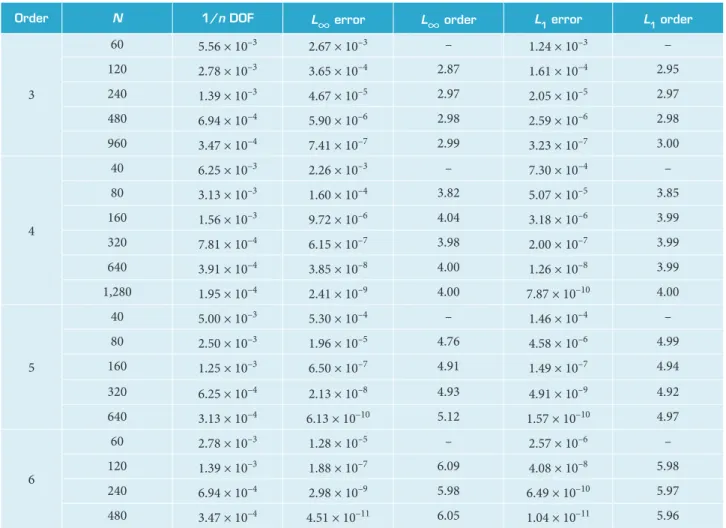
he same problem is simulated with the Gauss-Lobatto point distributions and the results are presented in Table 2. For the 2nd-order scheme, the Gauss-Lobatto point is actually in the middle of the domain, resulting in an equidistant CV partition, and therefore the corresponding results are not shown in Table 2.
Figure 5. Accuracy assessment of the 1-D SFV method for the linear scalar advection equation. Effect of equidistant (E) and
Gauss-Lobatto (GL) CV partition. Error shown in the L∞ norm.
10-10
E
rr
or
1/nDOF
10-8
10-4 10-3 10-2
SV3 - E SV3 - GL SV4 - E SV4 - GL SV5 - E SV5 - GL
10-6 10-4 10-2 be visualized in graphical form in Fig. 5. h e results shown in
this i gure refer to error measured in the L∞ norm.
h e next test case addressed considers the linear advection of a Gaussian pulse. Hence, a pulse with a half width equal to 0.05 dimensionless units is used as initial condition:
Table 2. Accuracy assessment of the 1-D SFV method for the linear scalar advection equation. Gauss-Lobatto CV partition.
Order N 1/n DOF L
∞
error L∞
order L1 error L1 order3
60 5.56 × 10⁻³ 2.67 × 10⁻³ – 1.24 × 10⁻³ –
120 2.78 × 10⁻³ 3.65 × 10⁻⁴ 2.87 1.61 × 10⁻⁴ 2.95
240 1.39 × 10⁻³ 4.67 × 10⁻⁵ 2.97 2.05 × 10⁻⁵ 2.97
480 6.94 × 10⁻⁴ 5.90 × 10⁻⁶ 2.98 2.59 × 10⁻⁶ 2.98
960 3.47 × 10⁻⁴ 7.41 × 10⁻⁷ 2.99 3.23 × 10⁻⁷ 3.00
4
40 6.25 × 10⁻³ 2.26 × 10⁻³ – 7.30 × 10⁻⁴ –
80 3.13 × 10⁻³ 1.60 × 10⁻⁴ 3.82 5.07 × 10⁻⁵ 3.85
160 1.56 × 10⁻³ 9.72 × 10⁻⁶ 4.04 3.18 × 10⁻⁶ 3.99
320 7.81 × 10⁻⁴ 6.15 × 10⁻⁷ 3.98 2.00 × 10⁻⁷ 3.99
640 3.91 × 10⁻⁴ 3.85 × 10⁻⁸ 4.00 1.26 × 10⁻⁸ 3.99
1,280 1.95 × 10⁻⁴ 2.41 × 10⁻⁹ 4.00 7.87 × 10⁻¹⁰ 4.00
5
40 5.00 × 10⁻³ 5.30 × 10⁻⁴ – 1.46 × 10⁻⁴ –
80 2.50 × 10⁻³ 1.96 × 10⁻⁵ 4.76 4.58 × 10⁻⁶ 4.99
160 1.25 × 10⁻³ 6.50 × 10⁻⁷ 4.91 1.49 × 10⁻⁷ 4.94
320 6.25 × 10⁻⁴ 2.13 × 10⁻⁸ 4.93 4.91 × 10⁻⁹ 4.92
640 3.13 × 10⁻⁴ 6.13 × 10⁻¹⁰ 5.12 1.57 × 10⁻¹⁰ 4.97
6
60 2.78 × 10⁻³ 1.28 × 10⁻⁵ – 2.57 × 10⁻⁶ –
120 1.39 × 10⁻³ 1.88 × 10⁻⁷ 6.09 4.08 × 10⁻⁸ 5.98
240 6.94 × 10⁻⁴ 2.98 × 10⁻⁹ 5.98 6.49 × 10⁻¹⁰ 5.97
480 3.47 × 10⁻⁴ 4.51 × 10⁻¹¹ 6.05 1.04 × 10⁻¹¹ 5.96
(53)
The linear advection problem again assumes periodic boundary conditions. h e simulation is carried out for various orders of accuracy, k = 1, 2, 3, 4 and 6, and up to a i nal time t = 2 dimensionless units. h e Gauss-Lobatto point distribution is used for CV partitioning.
Figure 6 shows the analytical and numerical solution proi les for a grid with 100 SVs. h e 1st-order simulation smeared the pulse so much that it is hardly recognizable. h is is due to the extra amount of dissipation associated with such low-order scheme. h e 2nd-order simulation retained the shape of the initial condition, but also smeared
Figure 6. Simulation of a travelling Gaussian pulse with SFV
schemes of various orders at t = 2 dimensionless units.
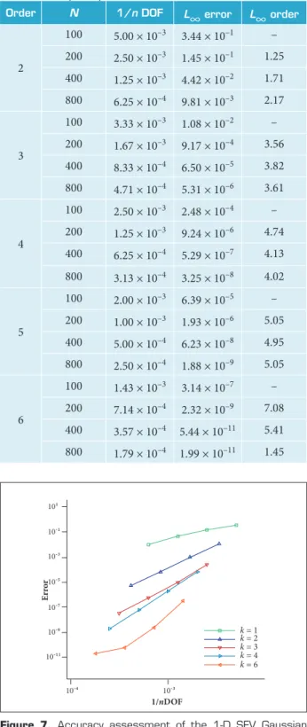
Figure 7. Accuracy assessment of the 1-D SFV Gaussian
pulse. Error shown in the L∞ norm.
x
u
0 0.2 0.4 0.6 0.8 1
0 0.2 0.4 0.6 0.8 1 Analytical k = 1 k = 2 k = 3 k = 4 k = 6
t = 2.0
0.6
0.2 0.4 0.8
0.2 0.4 0.6 0.8
0 1
t = 2
Analytical k = 1 k = 2 k = 3 k = 4 k = 6
0 1 u x E rr or
1/nDOF
10-4 10-3 10-11 10-9 10-7 10-5 10-3 10-1 101
k = 1 k = 2 k = 3 k = 4 k = 6 4th- and 6th-order simulations yield good results, which are very
similar to the analytical solution shown in the i gure.
Table 3 shows the error and order measured from the numerical experiment. Figure 7 shows graphically the table data. One can observe that the design order is obtained considering the Gauss-Lobatto CV partition scheme. As the order of the method increases, the error is consistently reduced to machine zero. It is worth mentioning that the limiter is enabled for these simulations and it can be observed that it is not activated for such smooth solutions. Another qualitative test case, which addresses a combination of smooth and discontinuous proi les, as in Krivodonova (2007), is also performed to check the SFV method capabilities. h e advected signal consists of a smooth Gaussian pulse, a square pulse, a triangle and half an ellipse, which are dei ned in the domain −1 ≤ x ≤ 1.
Hence, the problem initial condition is dei ned as:
Table 3. Accuracy assessment of the 1-D SFV method for the Gaussian pulse problem.
Order N 1/n DOF L
∞
error L∞
order2
100 5.00 × 10⁻³ 3.44 × 10⁻¹ –
200 2.50 × 10⁻³ 1.45 × 10⁻¹ 1.25
400 1.25 × 10⁻³ 4.42 × 10⁻² 1.71
800 6.25 × 10⁻⁴ 9.81 × 10⁻³ 2.17
3
100 3.33 × 10⁻³ 1.08 × 10⁻² –
200 1.67 × 10⁻³ 9.17 × 10⁻⁴ 3.56
400 8.33 × 10⁻⁴ 6.50 × 10⁻⁵ 3.82
800 4.71 × 10⁻⁴ 5.31 × 10⁻⁶ 3.61
4
100 2.50 × 10⁻³ 2.48 × 10⁻⁴ –
200 1.25 × 10⁻³ 9.24 × 10⁻⁶ 4.74
400 6.25 × 10⁻⁴ 5.29 × 10⁻⁷ 4.13
800 3.13 × 10⁻⁴ 3.25 × 10⁻⁸ 4.02
5
100 2.00 × 10⁻³ 6.39 × 10⁻⁵ –
200 1.00 × 10⁻³ 1.93 × 10⁻⁶ 5.05
400 5.00 × 10⁻⁴ 6.23 × 10⁻⁸ 4.95
800 2.50 × 10⁻⁴ 1.88 × 10⁻⁹ 5.05
6
100 1.43 × 10⁻³ 3.14 × 10⁻⁷ –
200 7.14 × 10⁻⁴ 2.32 × 10⁻⁹ 7.08
400 3.57 × 10⁻⁴ 5.44 × 10⁻¹¹ 5.41
800 1.79 × 10⁻⁴ 1.99 × 10⁻¹¹ 1.45
Δt are used as in the previous case. The simulation is carried
out with various orders of accuracy, for k = 2, 3, 4 and 6, up to a final time t = 2 dimensionless time units. The limiter
(54) with
where a = 0.5, z = 0.7, δ = 0.005, α = 10 and β = log 2/36 δ2.
0.6 0.2 0.4 0.8 1.2 0.2 -0.2 -0.2 -0.6 -0.8 -0.4
-1 0 0.4 0.6 0.8 1
1 0 u x 0.6 0.2 0.4 0.8 1.2 0.2 -0.2 -0.2 -0.6 -0.8 -0.4
-1 0 0.4 0.6 0.8 1
1
0
u
x
k = 2 Analytical
k = 3 Analytical
Figure 8. Simulation of travelling discontinuous proiles with (a) 2nd-
and (b) 3rd-order SFV schemes at t = 2 dimensionless time units.
( a)
( b )
( a)
( b )
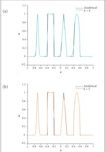
x x u u 1.2 1 1 -1 0.8 0.8 -0.8 0.6 0.6 -0.6 0.4 0.4 -0.4 0.2 0.2 -0.2 0 0 1 -1 -0.8 -0.6 -0.4 -0.2 0 0.2 0.4 0.6 0.8 -0.2 1.2 1 0.8 0.6 0.4 0.2 0 -0.2 Analytical k = 4
Analytical k = 5
but yields an approximation with no apparent oscillations and a better resolution before and ater such proiles. hese results indicate that high-order schemes tend to better resolve the analytical proile without numerical instabilities.
is enabled to test its ability to mark non-smooth states of the solution and reduce the oscillations observed in high-order interpolations. The results can be seen in Figs. 8 and 9, plotted for the CV mesh.
he 2nd-order case retains some of the initial features, but it signiicantly smears the proiles. No oscillations are noticeable due to the use of the limiter formulation. The 3rd-order solution resolves the Gaussian pulse with improved accuracy but there is a noticeable diference in the base of the discontinuous proiles. he same behavior is observed for the 4th-order solution with a tendency to better approach the peak numerical values. However, the result distances itself from the analytical one near steep gradients in the solution. Once again, no oscillations are observed in the numerical solution.
he 6th-order result achieves the better approximation with the analytical data. The smooth profiles are hardly distinguishable from the real solution. he reconstruction is not able to reproduce the triangle and square wave proiles exactly
Figure 9. Simulation of travelling discontinuous proiles with (a) 4th-
and (b) 6th-order SFV schemes at t = 2 dimensionless time units.
RINGLEB FLOW
he Ringleb low simulation consists of an external low, which has an analytical solution for the Euler equations derived with the hodograph transformation (Shapiro 1953). The analytical solution is used as initial condition for all simulations here discussed. he low depends on the inverse of the stream function, κ, and the velocity magnitude, v
t.
In the present simulations, these parameters are chosen as κ = 0.4 and 0.6, in order to deine the lateral boundaries of the domain, and v
t = 0.35 to deine the inlet and outlet boundaries.
of low regime, from supersonic to subsonic, for example, is shockless (Wang and Liu 2006).
In order to measure the order of the implemented SFV method, 4 meshes are considered for the grid reinement study, corresponding to 128; 512; 2,048 and 8,192 spectral volume cells. he analytical solution is computed for all meshes in order to measure how close the numerical results are to the exact solution. he error with respect to the analytical solution is computed using the L
1 and L ∞ norms of the density. Figure 10
shows the 2,048-cell grid and the Mach number contours computed in this grid with the 4th-order SFV method, using the corresponding high-order boundary representation.
he L
∞ norms of the error for the density values obtained
in the converged solutions with the 3rd- and 4th-order SFV method are shown in Fig. 11 for the 4 meshes considered. he igure indicates that the theoretical orders of accuracy are actually recovered by the simulations with the high-order boundary
representation. It should be pointed out that the same numerical test case was studied in Breviglieri e t a l . (2008), considering
only a linear boundary representation. It was observed in this efort that the low-order boundary treatment causes a shock wave to develop close to the inner boundary, which, then, makes the limiter active. Eventually, the shock wave propagates and it causes the simulation to diverge.
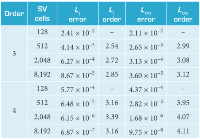
In the present paper, however, which considers the higher-order boundary representation, reasonable results are always obtained for this test case, including the simulations with the 4th-order SFV method. As previously discussed, for the 3rd-order scheme, a quadratic polynomial is used to represent the SV edges which lie along the domain boundaries. In a similar fashion, for the 4th-order scheme, a cubic polynomial is employed instead, which is compatible with the internal polynomial order of each SV. Table 4 presents the L
1 and L ∞
error norms of the density for the present calculations with the high-order boundary representation. The table also shows the actual measured order of accuracy for the 3rd- and 4th-order SFV methods. he orders of accuracy in the results shown in Table 4 are calculated as indicated in Wang and Liu (2006). he actual orders of accuracy here obtained are in good agreement with those shown in the cited reference.
Figure 10. Computational mesh and Mach number contours calculated with the 4th-order SFV method for the 2,048-cell grid.
Figure 11. Ringleb low error measurement with the 3rd- and
4th-order SFV method. Density error shown in the L∞ norm.
E
rr
or
1/sqrt(nDOF)
10-7
0.005 0.01 0.0150.02
10-3 10-2
3rd - order 4th - order
10-6 10-4 10-5 M ach 0.8 0.7 0.5 0.6 0.5 0.4 0.75 0.65 0.55 0.45 0.35
Table 4. Accuracy assessment of SFV method for the Ringleb low test case.
Order SV cells L1 error L1 order L
∞
error L∞
order 3128 2.41 × 10⁻² – 2.11 × 10⁻² –
512 4.14 × 10⁻³ 2.54 2.65 × 10⁻³ 2.99
2,048 6.27 × 10⁻⁴ 2.72 3.13 × 10⁻⁴ 3.08
8,192 8.67 × 10⁻⁵ 2.85 3.60 × 10⁻⁵ 3.12
4
128 5.77 × 10⁻⁴ – 4.37 × 10⁻⁴ –
512 6.48 × 10⁻⁵ 3.16 2.82 × 10⁻⁵ 3.95
2,048 6.15 × 10⁻⁶ 3.39 1.68 × 10⁻⁶ 4.07
8,192 6.87 × 10⁻⁷ 3.16 9.75 × 10⁻⁸ 4.11
NACA 0012 AIRFOIL
(a)
(b)
(a)
(b) airfoil surface. Both of these meshes are O -type grids
and they are presented in Fig. 12. The airfoil geometry is collapsed at the trailing edge. The far field boundary radius is 50 chord units. Differently from all other simulations in the present paper, the LU-SGS implicit time marching scheme, as discussed in Breviglieri et al. (2010b) and Parsani et al. (2010), is used for this test case. A CFL value of 1.0 × 10⁶ is
considered. The main objectives of the test case are to assess the SFV method accuracy and convergence for a transonic steady-state flow regime, as well as to provide further insight into the effects of a high-order boundary treatment.
The freestream flow replicates the conditions of the experimental data (McDevitt and Okuno 1985), that is, freestream Mach number of M∞ = 0.8 and 0 deg. angle-of-attack. Simulations with the 2nd-, 3rd- and 4th-order SFV schemes are performed, along with the 1st-order Roe scheme. Figure 13 presents density contours for the coarse mesh, for the 3rd-order SFV method solution and its comparison to the 1st-order Roe scheme. he 3rd-order low solution considers quadratic curved boundary reconstruction. he igure shows 30 evenly-spaced density contours, with values ranging from 0.8 to 1.6 in dimensionless density. A high-order post-processor tool would be necessary in order to accurately see and analyze these results. Nevertheless, one can already see that the 1st-order solution has clearly smeared out the shock wave that occurs in this low.
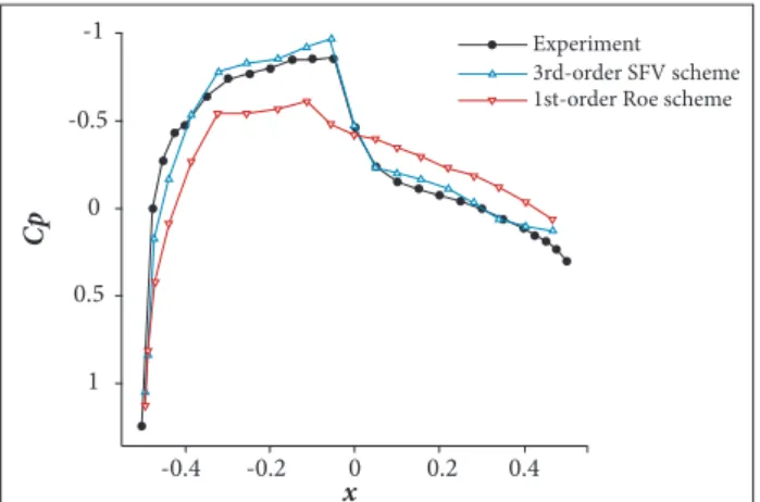
Figure 14 shows the corresponding pressure coeicient (Cp) distributions for the same mesh and for the same methods, as compared to the experimental data for this light condition. It is clear from the Cp distributions that the 1st-order scheme introduces too much dissipation and, essentially, smears out the shock wave, as already pointed out. he high-order Cp distribution, on the other hand, is remarkably close to the experimental results, particularly for the shock position and considering the crude geometric discretization.
hese results illustrate the potential of high-order methods to ease the burden on the mesh generation process for
Figure 12. Computational meshes used in the NACA 0012 simulations (a) Coarse mesh and (b) Fine mesh.
Figure 13. Evenly-spaced density contours on the coarse mesh: 30 contour lines are shown for dimensionless density values ranging from 0.8 to 1.6. (a ) 1st-order Roe scheme; (b) 3rd-order SFV scheme
Figure 14.Cp distributions for the coarse mesh solutions. 0
0
Cp
x
-0.5
-0.4 -0.2
0.5
0.2 0.4
-1
1
E x p e riment
(b) (a)
(c)
aeronautical applications. One should observe, however, that the experimental results consider the presence of the boundary layer and the consequent shock-boundary layer interaction that necessarily occurs in the experiment. For the numerical solution, the shock is typically captured as a sharper discontinuity, as one should expect for an Euler simulation. In this case, however, the high-order solution seems to follow exactly the experimental data due to the extremely coarse mesh used.
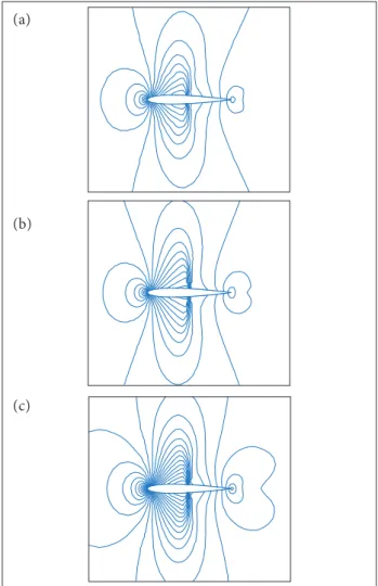
h e other set of results considers the i ne mesh. Figure 15 presents density contours for the same range of dimensionless density variation, as in the coarse grid simulations, for the 1st-order Roe method and for the 2nd- and 3rd-order SFV schemes. One can observe that the high-order solutions present much more features and sharper l ow gradients when compared
Figure 15. Evenly-spaced density contours on the i ne mesh: 30 contours are shown for dimensionless density varying from 0.8 to ranging from 0.8 to 1.6. (a) 1st-order Roe scheme; (b) 2nd-order SVF scheme; (c) 3rd-order SVF scheme
(55)
(56)
Figure 16. Entropy error for 3rd-order SFV method.
x E n tr o p y E rr o r
-0.6 -0.4 -0.2 0 0.2 0.4 0.6
0.01 0.015 0.02 0.025 0.03 0.035 0.04 0.045 0.05 0 x E nt rop y er ro r -0.4
-0.6 -0.2 0.2
0.02 0.225 0.215 0.035 0.045 0.05 SFV 3 SFV 3 curved
0.04
0.03
0.01
0.4 0.6
to the 1st-order method, mainly in the vicinity of the shock wave. h ese results coni rm the higher accuracy and resolution of the SFV methods, even though a limiter is used.
Another relevant simulation is performed to assess the benefits of the curved boundary implementation, namely, the measure of entropy error Єs levels at the airfoil boundary.
Since the diffusive flux vectors are 0, there is no physical dissipation mechanism that produces heat in regions of smooth l ow, away from shocks. If no external heat is added into the l ow, then it is adiabatic. Hence, from the i rst law of thermodynamics, it follows that entropy, given by
is constant throughout the field if no shocks are present. h erefore, the entropy error Єs, dei ned as
is a good measure of the accuracy of a numerical solution of the Euler equations.
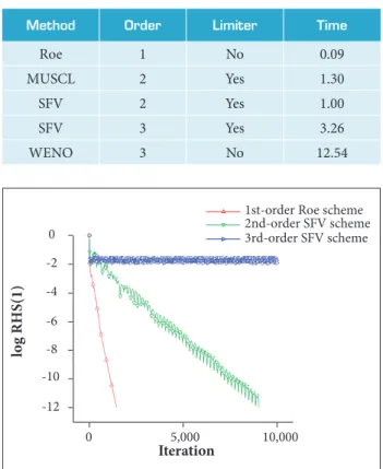
Figure 17 presents the convergence history for the simulations here considered in terms of the L∞ norm of the continuity equation residue. h e convergence history stalls for the SFV method, due to the presence of the limiter. h is behavior is typical of solutions which use non-linear limiters (Venkatakrishnan 1995).
Nevertheless, the simulations have reached a steady level, based on the force coei cients. Moreover, Table 5 shows the relative costs of the different methods, normalized by the 2nd-order SFV method. h e costs are measured on the i ne mesh simulations and provide an overall estimate of the iteration cost associated with high-order solutions. One should observe that the 3rd-order WENO simulation is approximately 4 times more demanding than the 3rd-order SFV scheme. h is increase in cost is associated with the dynamic stencil computation characteristic of the WENO solution, whereas the SFV method uses a static computational stencil throughout the simulation.
10, 000 5, 000
0 0
-2
-4
-6
-8
-10
-12
Iteration
lo
g RHS(1)
1st-order Roe scheme 2nd-order SFV scheme 3 rd-order SFV scheme
i nite-dif erence methods, but the results are not comparable to the later studies owing to their low resolution and parametric dif erences. h e forward step test case is designed to resolve complex oblique shock rel ections, pertinent to supersonic variable-geometry jet engine intakes. Due to computational constraints faced by Emery (1968), the test case was designed to be numerically simple to set up. h e initial conditions are uniform throughout the domain, and the inlet boundary condition is supersonic. Such setup is actually difficult to perform experimentally, due to the unrealistic combination of initial and boundary conditions. However, quantitative results are available for a range of numerical methods (Woodward and Colella 1984), which makes this a good test case for validating the capabilities of the present l ow solver, independently of the numerical method used.
h e artii cial nature of the test setup helps to evaluate the robustness of the spatial discretization algorithm combined with the limiter technique. Due to the strong shock rel ectionat the lower face of the step during the i rst few iterations, it is dii cult to maintain positivity of pressure and density using various numerical schemes. Furthermore, the edge of the forward step is a singular point of the Prandtl-Meyer expansion fan generated by the l ow over the step. h e continuity and momentum equations can disobey the second law of thermodynamics through an expansion fan. h is introduces numerical dii culty in the form of a nonphysical expansion shock, which at high Mach numbers and small cell sizes can yield negative pressures and densities in the code. h e MUSCL reconstruction, for the 2nd-order Roe scheme, for instance, is not able to produce a solution as the simulation diverges at er t = 1.0 dimensionless time units.
The 2-D configuration is 3 dimensionless length units long and 1 unit wide, with a step of 0.2 units high located at 0.6 units from the coni guration inlet. h e inl ow and outl ow boundary conditions are both supersonic, so the solver does not have to account for waves leaving the domain at the entrance boundary, or entering the domain at the exit boundary. Initially, the l ow is at M = 3 everywhere. As stated in the seminal study of Woodward and Colella (1984), this “admittedly artii cial” initial condition makes the problem very easy to set up. Since no physical constants or parameters, such as viscosity, are involved in the Euler equations, space and time units can be eliminated without the need for a dimensionless constant, and the l ow is driven by pressure and density ratios. h e simulation is run until t = 4.0 dimensionless time units, and the resulting shock wave pattern is examined. Two meshes are considered Figure 17. Convergence history for the Roe and SFV schemes.
Table 5. Iteration cost estimates.
Method Order Limiter Time
Roe 1 No 0.09
MUSCL 2 Yes 1.30
SFV 2 Yes 1.00
SFV 3 Yes 3.26
WENO 3 No 12.54
FORWARD FACING STEP
for this simulation, a coarse and a i ne one. h ese meshes are shown in Fig. 18. h e coarse mesh has a characteristic length
h = 1/40, and it has 8,272 cells and 4,134 nodes. h e i ner mesh
has 49,304 cells and 24,650 nodes, as well as a characteristic length h = 1/100. Further visualization of the mesh rei nement
can be seen in Fig. 19, which shows both the coarse and i ne
meshes for the region of the step. h is last i gure allows for a better visualization of the level of mesh rei nement in both cases.
For the present simulations, the 1st-order Roe method is considered along with the 2nd- and 3rd-order SFV methods. A total variation bounded (TVB) minmod limiter (Shu 1987) is considered in the present study for the 2nd-order SFV scheme in
Figure 19. Detail of the domain discretization for the step region. (a) Coarse Mesh; (b) Fine mesh.
Figure 18. Computational meshes used in the forward facing step coni guration simulations. (a) Coarse Mesh; (b) Fine mesh.
(b) (b)
order to compare the results with the proposed hierarchical limiter for the 3rd-order SFV method. Note that, for a 2nd-order scheme, the hierarchical limiter would reduce the local reconstruction order to 1st-order accuracy anyway. Density contours for the coarse mesh can be seen in Figs. 20, 21 and 22, respectively, for the cited methods. hirty evenly-spaced density contour lines
Figure 20. Density contours on the coarse mesh for the 1st-order Roe scheme. Figure shows 30 evenly-spaced dimensionless density contour lines from 0.1 to 4.6.
are presented, for dimensionless density values ranging from 0.1 to 4.6. One can observe that the SFV schemes present a better resolution of the shear layer compared to the 1st-order method, as well as a slightly improved shock resolution.
In order to investigate the similarities with the 1st-order simulation, the limited cells for the 2nd- and 3rd-order SFV
Figure 21. Density contours on the coarse mesh for the 2nd-order SFV scheme with the TVB limiter. Figure shows 30 evenly-spaced dimensionless density contour lines from 0.1 to 4.6.
s chemes are presented in Figs. 23 and 24. hese igures show the cells in which pressure reconstruction was performed at the last time step. For the 2nd-order method, there are too many cells limited by the TVB limiter, drastically reducing the overall solution reconstruction order. For the 3rd-order case, in which the hierarchical limiter is applied, the number of cells marked for limiting is reduced signiicantly. his conirms the superior behavior of the proposed limiting technique for the SFV method.
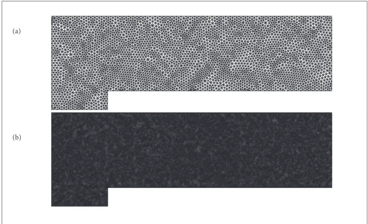
he next set of results considers the ine mesh. It is worth mentioning that the actual mesh used in the 3rd-order SFV method simulation has 295,824 control volumes, i.e., 6 times more cells than used in the 1st-order Roe and 3rd-order WENO simulation, because the reconstruction procedure subdivides each original cell, or spectral volume, into 6 new control volumes. his increases the overall simulation costs as reported in Table 6, where the relative computational costs are normalized by those of the 2nd-order SFV scheme. Furthermore, the reader can observe that the 3rd-order WENO simulation is about twice as costly as the 3rd-order SFV scheme. In the present test case, the hierarchical limiter formulation of the SFV method yields a reduction in the cost diferences between the present SFV
schemes and the WENO solution, in comparison, for instance, with the results observed for the NACA 0012 test case, shown in Table 5. It happens that, due to the unsteady nature of the present problem, the limiter is activated diferently at each time step and such behavior causes a penalty in the time step costs of both 2nd- and 3rd-order SFV results.
It is important to observe that, since the 2nd-order SFV method presents a large amount of limited cells due to the TVB limiter formulation, its results are actually representative of a 1st-order scheme. Hence, no results are shown for the ine mesh. Figure 25 shows the dimensionless density contours for the 1st-order Roe and 3rd-order SFV method simulations. Both
Figure 23. Limited cells for pressure reconstruction at the last time step for the 2nd-order SFV method with the TVB limiter.
Figure 24. Limited cells for pressure reconstruction at the last time step for the 3rd-order SFV method with the hierarchical limiter.
Table 6. Cost estimates per time step for the ine mesh.
Method Order Limiter Time
Roe 1 No 0.08
MUSCL 2 Yes 0.25
SFV 2 Yes 1.00
SFV 3 Yes 4.79
schemes present a sharp shock resolution, but the SFV method results seem to better capture other low features such as the shear layer. Again, the limited cells for pressure and internal energy
reconstruction at the inal time step are shown, respectively, in Figs. 26a and 26b for the 3rd-order SFV method calculations. One can clearly see that the high-order reconstruction is indeed
Figure 25. Density contours on the ine mesh for the 1st-order Roe scheme (a) and 3rd-order SFV scheme (b) . Thirty evenly-spaced contour lines for dimensionless density from 0.1 to 4.6.
Figure 26 . Limited cells for pressure (a) and internal energy (b) reconstructions at the last time step for the 3rd-order SFV method with the hierarchical limiter on the ine mesh.
(b)
(b) (a)
happening for the cells away from the discontinuities, since the limiter is only active at the discontinuities themselves.
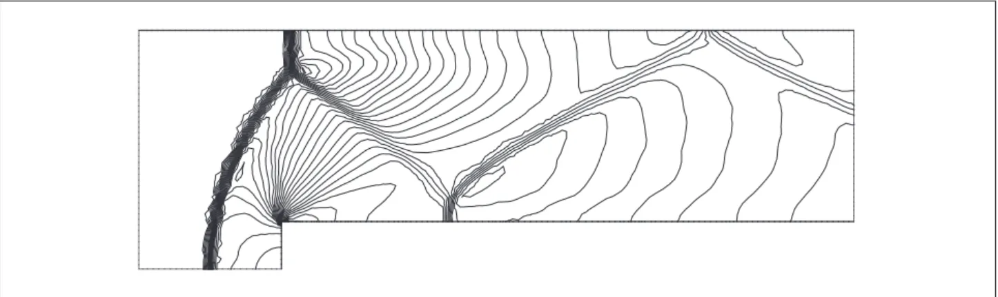
Finally, the 3rd-order method solution is plotted in Fig. 27 in terms of the density contours at the CV mesh. It is important to understand that this visualization considers data for the CV cells and, therefore, it better represents the actual resolution capabilities of the SFV method. Such deinition could be shown in the SV mesh but current visualization tools do not support high-order data visualization. A high-order post-processor would be necessary in order to allow a visualization with this level of resolution at the original SV mesh. Nevertheless, the level of resolution of low features is improved over the original SV mesh.
DOUBLE MACH REFLECTION
his problem is also a standard test case for high-resolution schemes (Woodward and Colella 1984), and it has been extensively studied by many researchers (Cockburn and Shu 1989; Wang et al. 2004). he physical problem is that of a right-moving M∞ = 10 shock wave, perpendicular to the axis of a 30 deg. half-angle wedge, which hits the tip of the wedge at time t = 0. Hence, the computational domain for the problem is chosen to be a rectangular region in the intervals [0, 4] × [0, 1], in the x- and y-directions, respectively. Initially, the right-moving M∞ = 10 shock is positioned at x = 1/6, y = 0 and makes a 60 deg. angle with the x-axis. For the bottom boundary, the exact post-shock conditions are imposed, through the Rankine-Hugoniot relations, for the region from x = 0 to x = 1/6, and a solid wall boundary condition is used for the rest of the lower domain boundary. For the top boundary, the solution is set to describe the exact motion of the M∞ = 10 shock. he let boundary is again set as the exact post-shock conditions, while the right boundary is set as an outlow boundary.
Two meshes are considered for this study, a coarse and a ine grid. he coarse mesh has 3,619 triangular cells, 1,808 nodes and characteristic dimensionless length h = 1/20. he ine mesh has 122,941 cells, 61,469 nodes and characteristic length of h = 1/120. Both meshes are shown in Fig. 28. It is interesting to mention that, for the SFV method simulations, the total number of CVs in the fine mesh turn out to be 368,823 and 737,646, respectively, for the 2nd- and 3rd-order methods. For the coarse mesh, the 1st-order Roe method is used, along with the 2nd- and 3rd-order SFV method. For the ine mesh, only the 1st-order Roe and 3rd-order SFV method simulations are reported here. For this test case, for instance, the 2nd-order MUSCL-reconstructed Roe scheme, with TVB minmod limiter, was not able to produce a solution. Negative values of pressure and density are found within the computation domain and the simulation diverges. his test case is a diicult one, in the sense that it requires proper boundary speciication, on a per-face basis, and it also features a low with a high level of kinetic energy.
Figure 29 presents numerical density contours for the coarse mesh, using the 1st-order Roe, 2nd- and 3rd-order SFV schemes, Moreover, 30 evenly-spaced contours are shown in each case and the dimensionless density values range from 1.25 to 21.5. For the mesh considered in this study, there is not much difference between the results. It is possible to note, however, that the Mach stem region, to the right end of the images, seems to be better defined for the SFV methods. For such problem, the use of limiters is obviously necessary. Figure 30 presents the limited cells for pressure reconstruction at the final time step for the 3rd-order SFV method. Clearly, only the shock region is indeed marked for limitation, as expected. Although necessary to obtain a numerical solution, the limiter utilization essentially reduces
Table 7. Estimates of relative costs per time step.
Method Order Limiter Time
Roe 1 No 0.04
MUSCL 2 Yes –
SFV 2 Yes 1.00
SFV 3 Yes 3.48
WENO 3 No 5.32
Figure 28. Computational meshes used for the double Mach relection problem simulations. (a) Coarse mesh; (b) Fine mesh.
the high-order resolution in such regions and it might be responsible for the similarities in the results with the low-order scheme.
Results considering the ine mesh are shown in Figs. 31 which presents dimensionless density contours in the same range used to report the results for the coarse grid. As before, 30 evenly-spaced contours are shown in each case. Clearly, there is much more resolution now, even with the 1st-order method. he shock waves have much improved resolution and the Mach stem corner presents more details than with the coarse mesh simulations. he numerical solution on the ine mesh with the 3rd-order SFV method seems to have spurious oscillations, as one can see in Fig. 31b. he shock waves are clearly better resolved, but the rest of the domain solution seems quite oscillatory and disturbed.
In order to investigate this effect, the limited cells for pressure reconstruction at the last time step are plotted in Fig. 32. One can clearly see that a large number of cells has been selected for pressure limitation. The same behavior is observed for the other variables. This apparent oscillatory behavior has not been previously observed for other test cases and, therefore, the authors suspect that the limiter algorithm
has some limitations with regard to simulations with very high Mach numbers and very strong discontinuities.
Further visualization of the results can be seen in Fig. 33, which presents density contours for the solution with the 3rd-order SFV method, but seen at the CV mesh level, that is, with 737,646 cells. As in the previous test case, this visualization considers data for the CV cells across the domain and better represents the actual resolution capabilities of the SFV method. A very sharp main shock wave can be clearly seen in the results, but oscillations in the density distribution are also seen in the post-shock region. Finally, Table 7 shows the relative costs of the different methods, normalized by the 2nd-order SFV method results.
Figure 29. Density contours on the coarse mesh for the 1st-order Roe scheme (a); for 2nd-order SFV scheme(b); and for the 3rd-order SFV scheme (c). Figure shows 30 evenly-spaced dimensionless density contour lines in the range from 1.25 to 21.5.
Figure 30. Limited cells for pressure reconstruction at the last time step for the 3rd-order SFV method.
(b)
(c) (a)
Costs are measured on the coarse mesh simulations and provide an overall estimate of the computational
Figure 31. Density contours on the ine mesh for the 1st-order Roe scheme (a) and 3rd-order SFV scheme(b). Figure shows 30 evenly-spaced dimensionless density contour lines in the range from 1.25 to 21.5.
Figure 32. Limited cells for pressure reconstruction at the last time step for the 3rd-order SFV method on the ine mesh.
(b) (a)
expensive for this problem than the 3rd-order SFV method calculations, considering the same input data. The reader should observe that the hierarchical limiter is active only in the discontinuous region of the solution, as depicted in Fig. 30.
CONCLUDING REMARKS
The application of the high-order SFV method to steady and unsteady inviscid compressible flow simulations is presented. The paper also addresses the use of high-order
Figure 33. Density contours at the CV mesh level for the 3rd-order SFV method solution in the ine grid.
and unsteady, have been addressed in order to highlight such features.
The main focus of the paper has been on the complex transient problems that stress the numerical method ability to compute flows with strong discontinuities without numerical divergence. The results obtained in the present research for the forward-facing step and the double Mach reflection problems have indicated that the SFV method is able to cope with the strong shock waves and produce good solutions. For both test cases, however, it is clear that the limiter algorithm still has limitations with regard to simulations with very high Mach numbers and very strong discontinuities. It seems that small oscillations are still allowed at the main shock wave, and these are convected downstream by the high-order scheme. Finally, the computational costs of the present high-order implementation are rather modest when compared to the benefits in flow resolution which can be achieved.
ACKNOWLEDGEMENTS
he authors gratefully acknowledge the partial support for this research provided by Conselho Nacional de Desenvolvimento Cientíico e Tecnológico (CNPq), under the Research Grants No. 309985/2013-7, No. 400844/2014-1 and No. 443839/2014-0. his study is also supported by the Coordenação de Aper-feiçoamento de Pessoal de Nível Superior (CAPES), through a graduate scholarship for the irst author. he authors are also indebted to the partial inancial support received from Fundação de Amparo à Pesquisa do Estado de São Paulo (FAPESP), under the Research Grant No. 2013/07375-0.
AUTHOR’S CONTRIBUTION
All authors contributed equally for the development of the work reported in the present paper.
REFERENCES
Abgrall R (1994) On essentially non-oscillatory schemes on unstructured meshes: analysis and implementation. J Comput Phys 114(1):45-58. doi: 10.1006/jcph.1994.1148
Barth T, Frederickson P (1990) Higher order solution of the Euler equations on unstructured grids using quadratic reconstruction. Proceedings of the 28th AIAA Aerospace Sciences Meeting; Reno, USA.
Barth T, Jespersen D (1989) The design and application of upwind schemes on unstructured meshes. Proceedings of the 27th Aerospace Sciences Meeting and Exhibit; Reno, USA.
Bigarella EDV, Azevedo JLF (2007) Advanced eddy-viscosity and Reynolds-stress turbulence model simulations of aerospace applications. AIAA J 45(10):2369-2390. doi: 10.2514/1.29332
Bigarella EDV, Azevedo JLF (2012) A study of convective lux schemes for aerospace lows. J Braz Soc Mech Sci & Eng 34(3):314-329. doi: 10.1590/S1678-58782012000300012
Breviglieri C, Azevedo JLF, Basso E (2010a) An unstructured grid implementation of high-order spectral inite volume schemes. J Braz Soc Mech Sci & Eng 32:419-433. doi: 10.1590/S1678-58782010000500001
Breviglieri C, Azevedo JLF, Basso E, Souza MAF (2010b) Implicit high-order spectral inite volume method for inviscid compressible lows. AIAA J 48(10):2365-2376. doi: 10.2514/1.J050395