Bol. Ciênc. Geod., sec. Artigos, Curitiba, v. 22, no3, p.405-419, jul-set, 2016.
Article
REVISITING THE ROLE OF OBSERVATION SESSION DURATION ON
PRECISE POINT POSITIONING ACCURACY USING GIPSY/OASIS II
SOFTWARE
Rediscutindo o papel da duração da sessão de observação na acurácia do
Posicionamento por Ponto Preciso com uso do software GIPSY/Oasis II
Adem G. Hayal 1
D. Ugur Sanli 2
1Nevsehir Haci Bektas Veli University, Engineering and Architecture Faculty, Department of Geodesy and
Photogrammetry Engineering, Nevsehir, Turkey. Email: [email protected]
2Yildiz Technical University, Civil Engineering Faculty, Department of Geomatic Engineering, Istanbul,
Turkey. Email: [email protected]
Abstract:
The accuracy of GPS precise point positioning (PPP) was previously modelled as a function of
the observing session duration T. The NASA, JPL’s software GIPSY OASIS II (GOA-II) along
with the legacy products was used to process the GPS data. The original accuracy model is not applicable anymore because JPL started releasing its products using new modelling and analysis strategies as of August 2007, and the legacy products are no longer available. The developments mainly comprise the new orbit and clock determination strategy, second order ionosphere modelling, and single station ambiguity resolution. Previously, the PPP accuracy was studied using v 4.0 of the GOA-II. The accuracy model showed coarser results compared to that of the relative positioning. Here, we processed the data of the International GNSS Service (IGS) stations to refine the accuracy of GOA-II PPP from version 6.3. Considering the above changes we refined the accuracy of PPP. First we modified the previous model used for the accuracy assessment. Then we tested out this model using straightforward polynomial and logarithmic models. The tests indicate the previous formulation still satisfactorily models the accuracy using refined coefficient values Sn = 7.8 mm , Se = 6.8 mm , Sv = 29.9 mm for T≥
2 h.
Keywords: GPS accuracy, Precise Point Positioning, GIPSY OASIS II, observing session duration.
Resumo:
Bol. Ciênc. Geod., sec. Artigos, Curitiba, v. 22, no,3 p.405-419, jul-set, 2016. GPS foram empregados os softwares GIPSY OASIS II (GOA-II) da JPL/NASA. Como a JPL passou a usar uma modelagem e novas estratégias de análises, o modelo convencional não é mais aplicável. A nova modelagem aborda, principalmente, novas órbitas e estratégias de determinação dos relógios dos satélites, modelagem de segunda ordem da ionosfera, e uma resolução única de ambiguidade. A acurácia do PPP foi previamente estudada usando a versão 4.0 do GOA-II. A acurácia do modelo mostrou resultados grosseiros comparados ao posicionamento relativo. Neste trabalho, foram processados os dados do serviço da estação internacional GNSS (IGS) para refinar a acurácia do GOA-II no modo PPP. Primeiramente, foram modificados os modelos prévios usados para avaliação da acurácia. Em seguida, os modelos foram testados empregando funções polinomiais simples e modelos logarítmicos. Os resultados mostraram que a formulação prévia ainda modela satisfatoriamente a acurácia usando os seguintes valores de coeficientes refinados: Sn = 7.8 mm , Se = 6.8 mm , Sv =
29.9 mm para T≥ 2 h.
Palavras-chave: acuracidade GPS, Posicionamento por Ponto Preciso, GIPSY OASIS II, duração da sessão de observação.
1. Introduction
Researchers and practitioners would like to know about the accuracy of GPS. This is needed for the accurate determination of deformation rates (Akarsu et al., 2015) and hence for survey planning. The use of PPP in real time GPS applications such as early prediction of earthquakes recently gained importance (Write et al., 2012). From this point of view, it is useful to revise the achievable accuracy of PPP from well-established GPS software, GIPSY/OASIS II (GOA-II) (Webb and Zumberge, 1997).
Bol. Ciênc. Geod., sec. Artigos, Curitiba, v. 22, no3, p.405-419, jul-set, 2016. where Sn, Se, and Sv are the accuracies of position components north, east and vertical in mm. T is
the observing session duration.
Using the formulas of Eckl et al. (2001), one was able to plan their survey prior to the field work. However their accuracy model was only appropriate for predicting the accuracy for 4 through 24 h data sets. Soler et al. (2006) developed an additional model that predicts the accuracy of 1-3 h sessions. Then the resulting formulation was:
where s denotes the accuracy for short session durations; RMSo (cm) is the overall RMS for the double differenced ionosphere-free carrier phase observables for the three single baseline solutions; k take on the values 1 cm , 1 cm , and 3.7 cm for the north, east, and vertical components respectively; and p represents peak-to-peak errors along the north, east and vertical components (see Soler et al., 2006, for details).
Firuzabadi and King (2012) later on tested the effect of network geometry, i.e. distribution and number of network points, as well as the effect of observing session duration on the positioning accuracy. They found that the current IGS accuracy can only be achievable with 6 h of GPS data and 4 or more well distributed reference stations.
Bol. Ciênc. Geod., sec. Artigos, Curitiba, v. 22, no,3 p.405-419, jul-set, 2016. positioning. The technique is also computationally efficient in that station-wise processing enables the processing time growing linearly.
Witchayang and Segantine (1999) and Fard and Dare (2006) were among the initial attempts assessing the PPP GPS results from web based GIPSY/OASIS software. Sanli and Engin (2009) noted the fact that practical applications such as monitoring of the tectonic motion and earthquakes might necessitate working over longer baseline lengths considering the need for using GPS stations from far stable tectonic plates such as Eurasia. Thus, for this concern in mind they revisited the accuracy of GPS positioning using GOA-II software. However, they did not use the PPP module as described in Zumberge et al. (1997), besides they fixed the ambiguities between station pairs using the ambiguity resolution technique of Blewitt (1989). This procedure produced results similar to those of the relative positioning. Namely, the dependency to GPS baselines was in concern. The results indicated that the positioning accuracy for the baselines longer than 300 km was dependent on baseline lengths. They produced new accuracy formulas in which the accuracy was dependent both on the observation session and baseline length:
where L represents the baseline length between GPS stations.
Sanli and Tekic (2010) made an attempt to model (i.e. to formulate) the accuracy of GOA-II PPP applying ordinary PPP processing, and they did not fix ambiguities between station pairs. The results were produced based on JPL’s legacy products (i.e. precise orbits, clocks, earth orientation parameters, etc. which were produced prior to the release of the new and improved products based on enhanced modelling and analysis procedures). The version 4.0 of GOA-II software was used for the data processing. Unlike relative positioning; the RMS of the solutions from shorter sessions, especially the east and the vertical components, showed dependency on station latitude. Namely, as the unsigned station latitude became smaller, the RMS of the solutions became larger. However, they only produced a model in which the positioning accuracy is formulated as a function of observing session duration. This model does not produce realistic results today because legacy products are no longer available and the processing needs to be based on the new and improved products. The refinement of the available accuracy model is the first task of this study, and it will be discussed in Section 2, in detail.
As Sanli and Tekic (2010) were studying the accuracy of GOA-II PPP, a new improved orbit determination strategy was newly adopted by NASA, JPL. Furthermore, the models to eliminate the second order ionosphere, which might be effective on the positioning at equatorial latitudes, were not available among the GOA-II modules (Kedar et al., 2003). Then, a single station ambiguity solution by Bertiger et al. (2010) was introduced that mainly improved the accuracy of horizontal positioning. All these were structured starting from the GOA-II PPP version 5.0 onwards. These enhancements were not taken into account in the analysis of Sanli and Tekic (2010).
Bol. Ciênc. Geod., sec. Artigos, Curitiba, v. 22, no3, p.405-419, jul-set, 2016. formulation is replaced with straightforward polynomial and log functions. IGS stations used in the study are almost evenly scattered around the globe depending on the data availability at the time. Then, we carried out the experiment using 2008 GPS data as done in Sanli and Tekic (2010). This was necessary for a direct comparison because the ionospheric conditions in 2008 coincided with the last solar cycle minimum whereas the present day data collection period coincides with a solar cycle maximum. The latest version 6.3 of GOA-II software was used in the processing of the GPS data (Desai et al., 2014). This version embraces improvements in orbit modelling, ambiguity resolution and ionosphere modelling. To show the enhancements from the latest version of GOA-II PPP, the results produced in this study are compared with those of the PPP studies produced earlier.
2. Original Accuracy Modelling
First of all, as also stated in Eckl et al. (2001), the accuracy here is not assessed by comparing GPS results with the results obtained from other space techniques such as VLBI and SLR. We also do not assess the accuracy in comparison to other software. The accuracy pronounced here is obtained by comparing the solutions from short GPS observation sessions with those of 24 h sessions, assuming the best positioning accuracy and hence the corresponding result is obtained through using 24 h data. Hence, the average of 24 h solutions is taken as the truth for the computation of the RMS from solutions of the shorter observation sessions. Therefore here the term “accuracy” rather than “precision” is used in assessing PPP results statistically.
In this context, the accuracy of PPP from JPL legacy products using GOA-II 4.0 was previously formulated as in the following (Sanli and Tekic, 2010):
where Sn (φ, T) denotes the accuracy of the north position component in mm as a function of
station latitude φ in degrees and observation session length T in hours. The coefficients an, bn, cn, dn are derived through a least squares analysis (Eckl et al., 2001). Equation 4 also applies for the
position components east and vertical.
Sanli and Tekic (2010) noticed the effect of station latitude on positioning results, especially on short observation sessions (i.e. 1-4 h) however they only modelled PPP results from 6-24 h GPS. Therefore, only the coefficient a , i.e. the effect of observing session duration, was found to be significant for all three GPS coordinates north, east and vertical as a result of the least squares analysis. Hence the accuracy of GPS PPP was formulated as
Bol. Ciênc. Geod., sec. Artigos, Curitiba, v. 22, no,3 p.405-419, jul-set, 2016. We first tested the modelling of Sanli and Tekic (2010) in which the modelling was merely performed with respect to observation session duration leaving the latitudinal effect out of the scope of the study. In fact, Sanli and Tekic (2010) used a model similar to the one given in Eckl et al. (2001). The only difference was that in their formula the dependency on station latitudes rather than baseline lengths was considered. Note that since they were using an absolute positioning technique (PPP) their processing was affected by global disturbances such as ocean, atmospheric and ground water loading rather than local or regional ones as given in Eckl et al. (2001).
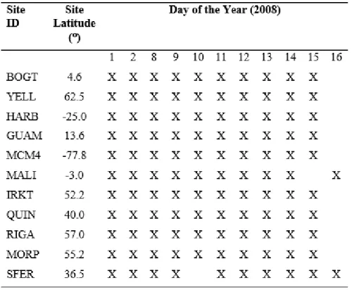
We used the same IGS stations and same GPS data as used in Sanli and Tekic (2010) as also mentioned before. Table 1 gives the schedule of these observations.
Table 1: Schedule of observations where X denotes that data from this day were included in the study.
3. PPP Processing
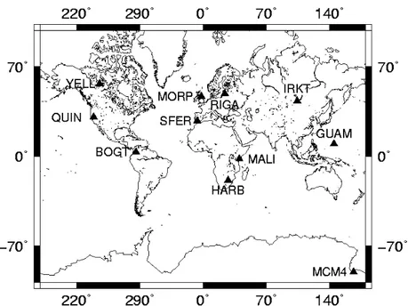
Bol. Ciênc. Geod., sec. Artigos, Curitiba, v. 22, no3, p.405-419, jul-set, 2016. Figure 1: Distributions of IGS permanent GPS stations used in the study.
With the motivation from the earlier studies we evaluated the effect of observing session duration on positioning solutions (Eckl et al., 2001; Sanli and Engin, 2009; Sanli and Tekic, 2010). In order to handle that, we sub-segmented 24 h observations into 1, 2, 3, 4, 6, 8, and 12 h sessions. From each session we computed a solution and then formed RMS values from the solutions of individual sub-sessions. The contaminated solutions, i.e. positional outliers, were removed using the most reliable robust outlier detection method ‘median’ as described in Tut et al. (2013). Solutions were also obtained from 24 h sessions and the average of those solutions was taken as the truth for computing the RMS of the shorter sessions.
The analysis of Sanli and Tekic (2010) did not include improvements from the NASA’s new orbit processing strategy. JPL stopped generating legacy orbits in August 2009. Sanli and Tekic (2010) analysis also did not account for the improvements due to new single station ambiguity resolution technique as developed by Bertiger et al. (2010). Furthermore, second order ionosphere effects were not taken into account since the related module based on the modelling of Kedar et al. (2003) was first released with the version 5.0.
Bol. Ciênc. Geod., sec. Artigos, Curitiba, v. 22, no,3 p.405-419, jul-set, 2016. variation (APV) maps were automatically applied following the IGS standards (Haines et al., 2010). Ocean loading corrections were also applied (Bos and Scherneck, 2015).
4. The New Accuracy Modelling
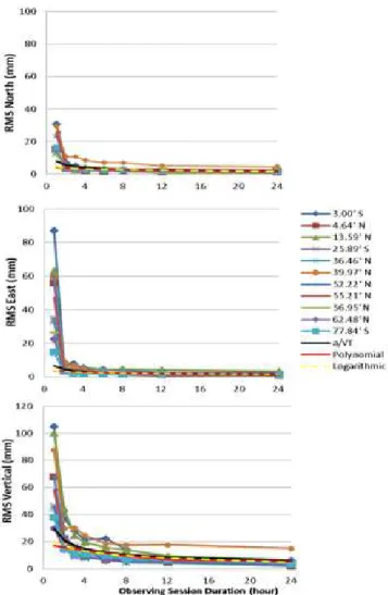
We first tested the mathematical model developed by Sanli and Tekic (2010) given with Equation 4 in Section 2. RMS values obtained from 24 h and all other sub-sessions for the GPS position components north, east and vertical are plotted against the observing session duration and given in Figure 2. Here note that as the observing session duration grows, the RMS of the solution becomes smaller. We will discuss later the meaning of the black, yellow, and red curves which are also superimposed on to the RMS values in Figure 2. The RMS values shown in Figure 2 were modelled for all three GPS position components north, east and vertical using the general relation given in Equation 4.
The improvement in JPL and IGS products led us also involve 4 h solutions in the modelling. Hence, differing from that of Sanli and Tekic (2010), which performed their modelling over 6-24 h session lengths, we performed our modelling using RMS values from 4-24 h solutions.
The coefficients a, b, c, and d for the each component was estimated using least squares. For the each constant of each GPS coordinate appearing in Equation 4, test statistics were formed by dividing the estimate to its formal error. These test statistics were then compared with the critical values obtained from Student’s t test for α = 0.05 significance level.
Bol. Ciênc. Geod., sec. Artigos, Curitiba, v. 22, no3, p.405-419, jul-set, 2016. Figure 2: Prediction/model fits to the RMS values of this study from observing session durations of 1 through 24 h (1-3 h period is just extrapolated). The model fit for the polynomial
is represented with solid red line, for the log function with a dashed yellow line, and for Sanli and Tekic (2010) model with a black line.
Table 2: Significant constants/estimates and their 1-sigma uncertainties from least squares analysis for position components north, east, and vertical.
Bol. Ciênc. Geod., sec. Artigos, Curitiba, v. 22, no,3 p.405-419, jul-set, 2016. where Sn, Se, Sv are the accuracy estimates and T is the observing session duration. Comparing
Equation 6 with Equation 5 reveals the improvement in the accuracy of GPS PPP mainly induced from JPL’s new orbit determination strategy, ambiguity resolution technique and 2nd order ionosphere modelling. Namely, the model coefficients in Equation.5 have improved about 42% for the north, 67% the east, and 27% for the vertical coordinates. The solid black curve with triangular markers superimposed through the RMS values in Figure 2 represents the model derived using Equation 6.
5. Discussion
5.1 Polynomial and Logarithmic Fitting
In this section, the accuracy of PPP will also be modelled using polynomial and logarithmic functions. This is because these functions are more straightforward, or less complicated than that of Sanli and Tekic (2010). In addition, Sanli and Tekic (2010) model only comprised the accuracy for the session durations of 4-24 h. Sessions 1-3 h in Figure 2 were only extrapolated. Note also that the segment of the solid black line fitting to 1 through 4 h sessions does not represent well the spectrum of the RMS. One reason in fitting polynomial and log functions to the RMS to test out whether or not an improvement could be gained in the modelling of shorter sessions.
The second order polynomial and a log function fitted into the RMS values of the north, east, and vertical coordinates were:
where P(T) and L(T) denote the RMS derived from the polynomial and logarithmic models respectively. Coefficients a0, a1, a2, a, and b are estimated through least squares analysis, and T
Bol. Ciênc. Geod., sec. Artigos, Curitiba, v. 22, no3, p.405-419, jul-set, 2016.
5.2 Internal Model Assessment
Table 3 compares the predicted model values with the mean RMS values obtained using the RMS values given in Figure 2. The comparisons are made for all three GPS coordinates north, east, and up. The model fit for the polynomial is represented with solid red line whereas the model fit for the log function is represented with a dashed yellow line in Figure 2.
Note that the polynomial and logarithmic models are only successful in predicting the accuracy of 4-24 h solutions. However, Sanli and Tekic (2010) model is able to predict 2-24 h solutions. On the other hand, all three models fail to predict the actual mean RMS of 1h solutions. The refined Sanli and Tekic (2010) model given with Equation 6 still appears to be the best model which satisfactorily predicts the mean RMS for 2-24 h sessions. Appendix, attachments, glossary, and additional material must be available preferably in PDF format in which it will be linked in the whole text. If this material is part of a file, it must be presented after the References and follow the same formatting instructions of the text.
Bol. Ciênc. Geod., sec. Artigos, Curitiba, v. 22, no,3 p.405-419, jul-set, 2016.
5.3 External Model Assessment
In this section we compare our 24 h predictions which are derived from Equation 6 with the evidence from previous studies. In addition, we also append the empirical evidence produced in this study and the current IGS positioning accuracies obtained from https://igscb.jpl.nasa.gov/ (Table 4).
Table 4: Comparison of the results from this study with those of the published work previously. Predictions of 24 h are compared.
It is clearly seen from the table that Sanli and Tekic (2010) prediction is the poorest of all in representing the empirical evidence produced in this study. Note that the prediction of the east component from Sanli and Tekic (2010) became much better with the single receiver ambiguity solution developed by Bertiger et al. (2010). The refined second order ionosphere model and the required backward reprocessing by the JPL, including the corrections also for GPS satellites, came along with the software release v 6.3. The above mentioned enhancements in the software were lacking in the analysis of Sanli and Tekic (2010). Also note that 3-4 mm horizontal and 12 mm vertical GIPSY positioning accuracies using the model developed here and using as short as 4 h sessions do not yet satisfy the IGS accuracy given in Table 4.
Furthermore, the IGS vertical positioning accuracy is not even satisfied with 12 h of data. Akarsu et al. (2015) showed that the positioning using short observation sessions also affect the velocities estimated. Users of GPS campaign measurements employing 8-12 h of observation sessions need to take this into consideration.
6. Conclusion
Bol. Ciênc. Geod., sec. Artigos, Curitiba, v. 22, no3, p.405-419, jul-set, 2016. polynomial and logarithmic functions. Comparisons from all three models revealed that with the refined model of Sanli and Tekic (2010), the accuracy can satisfactorily be predicted for session durations of 2 through 24 h. The accuracy estimated from the new model is comparable or shows improvement to those of the previous work. We assume the new model will be of interest to researchers who wish to plan their GPS campaigns prior to field works. As future work, we plan to include a non-linear coefficient c in our model (i.e. ) so that it might help improve the fit for 1 h sessions.
AKCNOWLEDGEMENT
We are grateful to NASA JPL for providing the license of GIPSY/OASIS II software. IGS has been doing a great service in providing various data and products. In this study we used the GPS data of the IGS using SOPAC servers, and we are grateful to SOPAC researchers as well. The authors would like to thank to Bahattin Erdogan for his kind help in determining positional outliers. Last but not least we are also thankful to the two anonymous reviewers who provided substantial contribution to the revision of the paper.
REFERENCES
Akarsu, V.; Sanli, D.U.; Arslan, E. “Accuracy of Velocities from Repeated GPS Measurements.”
Natural Hazards and Earth System Sciences 15 (2015): 875-884.
Altamimi, Z.; Collilieux, X.; Metivier, L. “ITRF08: An Improved Solution of the International Terrestrial Reference Frame.”Journal of Geodesy 85 (2011): 457-473.
Bertiger, W.; Desai, S.D.; Haines, B.; Harvey, N.; Moore, A. W.; Owen, S.; Weiss, J.P. “Single Receiver Phase Ambiguity Resolution with GPS Data.”Journal of Geodesy 84 (2010): 327–337. Blewitt, G. “Carrier Phase Ambiguity Resolution for the Global Positioning System Applied to Geodetic Baselines up to 2000 km.”Journal of Geophysical Research 94 (1989): 10187-10283. Blewitt, G. “Advances in Global Positioning System Technology for Geodynamics
Investigations 1978-1992.” Contributions of Space Geodesy to Geodynamics: Technology. (1993): 195-213.
Boehm, J.; Niell, A.; Tregoning, P.; Schuh, H. “Global Mapping Function (GMF): A New Empirical Mapping Function based on Numerical Weather Model Data.”Geophysical Research Letters 33 (2006): 1-4.
Bos, M.S.; Scherneck, H.G. “Ocean Tide Loading Provider.” Onsala Space Observatory, Chalmers University of Technology, Gothenburg, Sweden, Accessed July 5, 2015. http://holt.oso.chalmers.se/loading/
Davis, J.L.; Prescot W.H.; Svarc, J.; Wendt, K. “Assessment of Global Positioning
Measurements for Studies of Crustal Deformation.”Journal of Geophysical Research 94 (1989): 13635-13650.
Bol. Ciênc. Geod., sec. Artigos, Curitiba, v. 22, no,3 p.405-419, jul-set, 2016. Dong, D.N., and Bock, Y. “Global Positioning System Network Analysis with Phase Ambiguity Resolution Applied to Crustal Deformation Studies in California.”Journal of Geophysical Research 94 (1989): 3949-3966.
Eckl, M. C.; Snay, R. A.; Soler, T.; Cline, M. W.; Mader, G. L. “Accuracy of GPS-Derived Relative Positions as a Function of Inter-Station Distance and Observing-Session Duration.”
Journal of Geodesy 75 (2001): 633-640.
Feigl, K.L.; Agnew, D.C.; Bock, Y.; Dong, D.; Donellan, A.; Hager, B.H.; Herring, T.A.; Jakson, D.D.; Jordan, T.H.; King, R.W.; Larsen, S.; Larson, K.M.; Murray, M.H.; Shen, Z.K.; Webb, F.H. “Space Geodetic Measurement of Crustal Deformation in Central and Southern California, 1984-1992.”Journal of Geophysical Research, 98 (1993): 21677-21712.
Firuzabadi, D.; and King, R. W. “GPS Precision as a Function of Session Duration and Reference Frame using Multi-Point Software.”GPS Solutions 16 (2012): 191–196.
Ghoddousi-Fard, R.; Dare, P. “Online GPS Processing Services: an Initial Study.”GPS Solutions
10 (2006) 12-20.
Gurtner, W.; Beutler, G.; Botton, S.; Rothacher, M.; Geiger, A.; Kahle, H. G.; Schneider, D.; Wiget, A. “The use of the Global Positioning System in Mountainous Areas.”Manuscripta Geodaetica 14 (1989): 53-60.
Haines, B.; Bar-Sever, Y.; Bertiger, W.; Desai, S.; Weiss, J. “New Grace-based Estimates of the GPS Satellite Antenna Phase-and Group-Delay Variations.” Paper Presented at the Annual Meeting for the IGS Workshop, Newcastle upon Tyne, England, June 28- July 1, 2010. Heflin, M.B.; Bertiger, W.I.; Blewitt, G.; Freedman, A.P.; Hurst, K.J.; Lichten, S.M.;
Lindqwister, U.J.; Vigue, Y.; Webb, F.H.; Yunck, T.P.; Zumberge, J.F. “Global Geodesy using GPS without Fiducial Sites.”Geophysical Research Letters 19 (1992): 131-134.
Kedar, S.; Hajj, G. A.; Wilson, B. D.; Heflin, M. B. “The Effect of the Second Order GPS Ionospheric Correction on Receiver Positions.”Geophysical Research Letters 30 (2003): 1829. doi: 10.1029/2003GL017639.
Larson, K.M.; Agnew, D.C. “Application of the Global Positioning System to Crustal
Deformation Measurement, 1, Precision and Accuracy.”Journal of Geophysical Research 96 (1991): 16547-16565.
Petit, G., and Luzum, B., IERS Conventions (2010), No. IERS-TN-36. Bureau International des Poids et Mesures Sevres (France),2010.
Rius, A.; Juan, J.M.; Hernández-Pajares, M.; Madrigal, A.M. “Measuring Geocentric Radial Coordinates with a Non-Fiducial GPS Network.”Bulletin Géodésique 69 (1995): 320-328. Sanli, D. U.; Engin, C. “Accuracy of GPS Positioning over Regional Scales.”Survey Review
41(2009): 192-200.
Sanli, D.U.; and Tekic, S. Accuracy of GPS Precise Point Positioning: A Tool for GPS Accuracy Prediction. Saarbrücken: LAP Lambert Academic Publishing, 2010.
Soler, T.; Michalak, P.; Weston, N. D.; Snay, R. A.; Foote, R. H. “Accuracy of OPUS Solutions for 1- to 4-h Observing Sessions.”GPS Solutions 10 (2006): 45-55.
Bol. Ciênc. Geod., sec. Artigos, Curitiba, v. 22, no3, p.405-419, jul-set, 2016. Webb, F.H.;Zumberge, J.F. “An Introduction to GIPSY/OASIS-II.”A User Manual Prepared by Jet Propulsion Laboratory, Pasadena, CA, June 16-20, 1997.
Witchayangkoon, B.; Segantine, P.C.L. “Testing JPL’s PPP Service.”GPS Solutions 3 (1999): 73-76.
Wright, T. J.; Houlié, N.; Hildyard, M.; Iwabuchi, T. “Real-Time, Reliable Magnitudes for Large Earthquakes from 1 Hz GPS Precise Point Positioning: The 2011 Tohoku-Oki (Japan)
Earthquake.”Geophysical Research Letters 39 (2012): L12302. doi:10.1029/2012GL051894. Zumberge, J. F.; Heflin, M. B.; Jefferson, D. C.; Watkins, M. M.; Webb, F. H. “Precise Point Positioning for the Efficient and Robust Analysis of GPS Data from Large Networks.”Journal of Geophysical Research 102 (1997): 5005-5017.