www.ann-geophys.net/28/1571/2010/ doi:10.5194/angeo-28-1571-2010
© Author(s) 2010. CC Attribution 3.0 License.
Annales
Geophysicae
Accuracy analysis of the GPS instrumental bias estimated from
observations in middle and low latitudes
D. H. Zhang1,2, W. Zhang1,3, Q. Li1,4, L. Q. Shi5, Y. Q. Hao1, and Z. Xiao1
1Department of Geophysics, Peking University, Beijing, China
2State Key Laboratory of Space Weather, Chinese Academy of Sciences, Beijing, China
3Department of Geodesy and Geomatics Engineering, University of New Brunswick, Fredericton, New Brunswick, Canada 4Aviation Data and Communication Corporation, Beijing, China
5Center for Space Science and Applied Research, China Academic Science, Beijing, China
Received: 15 October 2009 – Revised: 4 July 2010 – Accepted: 20 July 2010 – Published: 25 August 2010
Abstract. With one bias estimation method, the latitude-related error distribution of instrumental biases estimated from the GPS observations in Chinese middle and low lat-itude region in 2004 is analyzed statistically. It is found that the error of GPS instrumental biases estimated under the assumption of a quiet ionosphere has an increasing ten-dency with the latitude decreasing. Besides the asymmetrical distribution of the plasmaspheric electron content, the obvi-ous spatial gradient of the ionospheric total electron content (TEC) along the meridional line that related to the Equa-torial Ionospheric Anomaly (EIA) is also considered to be responsible for this error increasing. The RMS of satellite instrumental biases estimated from mid-latitude GPS obser-vations in 2004 is around 1 TECU (1 TECU = 1016/m2), and the RMS of the receiver’s is around 2 TECU. Nevertheless, the RMS of satellite instrumental biases estimated from GPS observations near the EIA region is around 2 TECU, and the RMS of the receiver’s is around 3–4 TECU. The results demonstrate that the accuracy of the instrumental bias esti-mated using ionospheric condition is related to the receiver’s latitude with which ionosphere behaves a little differently. For the study of ionospheric morphology using the TEC de-rived from GPS data, in particular for the study of the weak ionospheric disturbance during some special geo-related nat-ural hazards, such as the earthquake and severe meteoro-logical disasters, the difference in the TEC accuracy over different latitude regions should be paid much attention. Keywords. Ionosphere (Equatorial ionosphere)
Correspondence to:D. H. Zhang ([email protected])
1 Introduction
The capability of dual carrier frequencies of GPS system to remove ionospheric delays provides a useful tool for mea-suring the ionospheric total electron content (TEC) (Lanyi and Roth, 1988; Coco et al., 1991). With the wide appli-cation of high-precision GPS technology, the GPS receiver has gradually become a routine and effective equipment for ionospheric measurements. The advantages of globally dis-tributed receivers and easy data availability make the col-lection of the ionospheric TEC derived from raw GPS ob-servations very convenient. Actually, like the ionospheric F layer critical frequency, foF2, obtained using ionosonde, the ionospheric TEC already becomes a basic ionospheric parameter to describe ionospheric behavior. Internet-shared and globally distributed GPS observations provide the world-wide researchers with a facility to study the local, regional and global ionosphere independently, quickly and simultane-ously. Research on ionospheric morphology and disturbance based on this parameter greatly extends our understanding for the ionospheric temporal and spatial variations (Ho et al., 1996; Mannucci et al., 1998; Mendillo, 2000; Zhang and Xiao, 2005).
that of the GPS signal delays caused by background iono-sphere. Therefore, only under the correct estimation of the instrumental biases, the analysis results of the ionospheric morphology based on TEC derived from GPS observations are believable. Nevertheless, as for most GPS users, it is very difficult or sometimes impossible to measure GPS in-strumental biases in real-time during the period of GPS op-eration. In order to derive the correct ionospheric TEC from raw GPS observations, a number of methods to estimate in-strumental biases have been developed under some assump-tions on ionospheric condition. To convert a slant path TEC to a vertical TEC, the ionosphere is assumed to be a thin shell encircling the Earth with an average ionospheric height that is usually set as constant value during TEC calculation from GPS observation. This assumption undoubtedly introduces error during the derivation process of vertical ionospheric TEC from GPS data. Another basic ionospheric condition assumes the ionospheric variation stable in the sun-fixed co-ordinate system, or the ionosphere should exhibit smooth temporal and spatial variation (Sardon et al., 1994; Sardon and Zarraoa, 1997; Ciraolo et al., 2007; Ma and Maruyama, 2003; Lunt et al., 1999). This assumption is satisfied in most situations, but in some special ionospheric conditions or in some special ionospheric regions, the error of this iono-spheric assumption is larger. Actually, some kind of severe disturbing phenomena can make the ionosphere deviate the average ionospheric status greatly. These disturbances can degrade the accuracy of the estimated instrumental biases and ionospheric TEC from GPS data based on the smooth ionospheric condition.
Ionospheric storm is one of the important ionospheric dis-turbing phenomena. During storm period, the ionosphere ex-hibits severe deviation from background ionosphere that lasts from several hours to several days and covers regionally or globally. Based on the GPS data observed in mid-latitude region from 2004 to 2006, the instrumental bias were ob-tained using a estimation method of instrumental bias, and the differences of the instrumental bias between the active geomagnetic days and the quiet geomagnetic days were stud-ied (Zhang et al., 2009a). It is found that the standard devia-tion of instrumental biases during active geomagnetic days is obviously larger than that during the quiet days, and this de-viation can degrade the accuracy of ionospheric TEC derived from GPS observations.
The significant effect of the asymmetrical distribution of the plasmaspheric electron content on the GPS instrumental bias estimation has been studied, and it is found that the accu-racy of ionospheric TEC increases if considering the plasma-spheric electron content meridional distribution during bias estimation (Lunt et al., 1999; Mazzella et al., 2002). Be-sides the latitude-related distribution of the plasmasphere, the ionospheric electron content also exhibits an obvious asym-metrical distribution along the meridional line related to the Equatorial Ionospheric Anomaly (EIA) that strongly controls the variation of the low latitude ionosphere. Comparing with
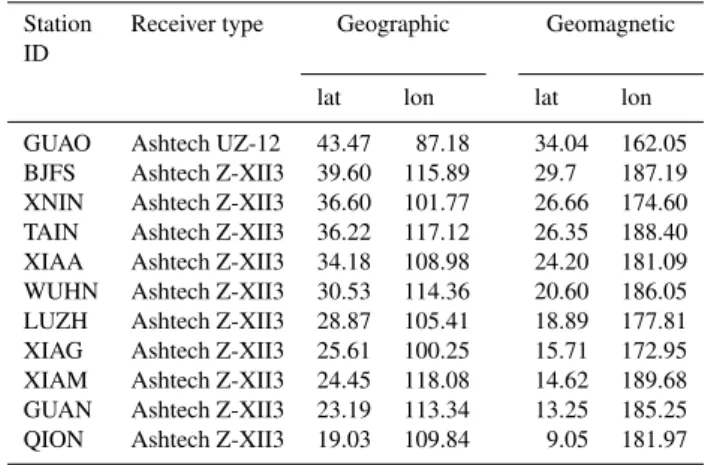
Table 1. Station ID, receiver types, geographic and geomagnetic latitude (lat) and longitude (lon) used in the paper.
Station Receiver type Geographic Geomagnetic ID
lat lon lat lon
GUAO Ashtech UZ-12 43.47 87.18 34.04 162.05 BJFS Ashtech Z-XII3 39.60 115.89 29.7 187.19 XNIN Ashtech Z-XII3 36.60 101.77 26.66 174.60 TAIN Ashtech Z-XII3 36.22 117.12 26.35 188.40 XIAA Ashtech Z-XII3 34.18 108.98 24.20 181.09 WUHN Ashtech Z-XII3 30.53 114.36 20.60 186.05 LUZH Ashtech Z-XII3 28.87 105.41 18.89 177.81 XIAG Ashtech Z-XII3 25.61 100.25 15.71 172.95 XIAM Ashtech Z-XII3 24.45 118.08 14.62 189.68 GUAN Ashtech Z-XII3 23.19 113.34 13.25 185.25 QION Ashtech Z-XII3 19.03 109.84 9.05 181.97
the mid-latitude ionosphere, the low latitude ionosphere ex-hibits greater spatial gradient and more intensive temporal variation, so it is more difficult to describe the ionospheric variations in this region. Therefore, the accuracy of GPS in-strumental biases estimated from low latitude GPS observa-tion based on the ionospheric model should be lower than that estimated from the mid-latitude data. Undoubtedly, a detailed quantitative analysis about the instrumental bias ac-curacy is useful for the correctly understanding of the iono-spheric TEC results. Recently, some accuracy analysis for the ionospheric TEC estimated from GPS observations over low latitudinal region has been reported (Niranjan et al., 2007; Mazzella et al., 2007; Thampi et al., 2007). In this paper, using the observations of the GPS receivers located in the middle and low latitude in China longitude sector in 2004, the statistical analysis for the instrumental biases esti-mated in different latitude will be studied. Additionally, the error range of the ionospheric TEC derived from GPS obser-vations in different latitude will be estimated based on the variation of the instrumental bias.
2 Data and method for the determination of GPS instrumental biases
Considering the possible influence of the ionospheric vari-ability during different solar cycle period on the accuracy of the instrumental bias estimation, the GPS data in solar mi-nimum year (2004) are selected. All the GPS stations are located in China longitude sector and in middle and low lati-tude. The GPS data are in RINEX format, and the sampling rate is 30 s. The GPS station ID, the type of the receivers, and the position of the stations are shown in Table 1.
The measurements of the pseudo-ranges and carrier phases in two L-band carrier frequencies (fL1=1575.42 MHz, fL2=1227.60 MHz) are included in GPS data. The
following equations, respectively (Mannucci et al., 1998; Ma and Maruyama, 2003):
Slant TECp= 2(f1f2) 2
k f12−f22(P2−P1) (1)
Slant TECl= 2(f1f2) 2
k f12−f22(L1λ1
−L2λ2) (2)
wherek=80.62 m3s−2,λ
1andλ2are the wavelength
corre-sponding to fL1, fL2, P1 and P2are the pseudo-range
mea-surments, and L1and L2are the carrier phase measurments
at fL1, fL2. Because of the potential ambiguity in the
car-rier phase measurement, the Slant TECl in Eq. (2) is only a relative slant TEC value. However, the relative error of the Slant TECl is much lower than that of the absolute TEC obtained from Eq. (1). In the actual application, combining the Slant TECl and the Slant TECp during one continuous tracking arc, the offset value Brsbetween the Slant TECland
the Slant TECpcan be calculated using Eq. (3), and the ab-solute slant TEC with higher accuracy in each observation epoch can be obtained from Eq. (4) (Mannucci et al., 1998; Ma and Maruyama, 2003).
Brs= PN
k=1 Slant TEC
p
k−Slant TEC l k
sin2elk
PN
k=1sin2elk
(3)
Slant TEC=Slant TECl+Brs (4)
whereN is the number of observation epochs during a con-tinuous tracking arc, elk is the satellite’s elevation angle, and the term sin2elk is a weighting factor for restraining the so-called signal multipath effect. As the pseudo-range with low elevation angle is apt to be affected by the multipath effect and the reliability decreases, consequently, the contribution to the Brs determination is greatly diminished from slant
paths with low elevations in Eq. (3). Thus, the absolute slant TECs, which are free of ambiguities and have low noise and multipath effects, can be obtained from Eq. (4) (Mannucci et al., 1998; Ma and Maruyama, 2003). In this study, the val-ues are restricted to satellite elevation angles larger than 30◦
. Considering the satellite and receiver instrumental biases, the vertical ionospheric TEC at the ionosphere pierce point (IPP) (the intersecting point between the line from the satellite to the receiver and the ionosphere shell) can be obtained by us-ing the followus-ing relation:
TEC=(Slant TEC−Bs−Br)cosEion (5)
whereBs andBr are the satellite and receiver instrumental biases, respectively. Eionis the mapping angle that can be obtained from Eq. (6):
Eion=arcsin
RE
RE+Hicos el
(6)
whereREis the mean radius of the Earth andHiis the height
of the ionospheric shell (assumed to be 400 km in this study). The instrumental biases (including satellite and receiver) and vertical TEC in Eq. (5) can be determined using the self-calibration of pseudo-range errors (SCORE) process (Lunt et al., 1999). The basic concept in the SCORE process is that when the IPP-derived line between two satellites and a receiver arrive at the same moment at a same point, that is, when a so-called conjunction occurs, the vertical TECs at the two IPP derived using Eq. (5) are assumed equality. It should be noted that this concept implies an ionospheric background model that the ionosphere over the same latitudi-nal zone has the same diurlatitudi-nal variation, or, the concept con-tains an assumption of the ionospheric condition with smooth spatial and temporal variation. For a certain data sample, as-suming Slant TECα(θα,τα)and Slant TECβ(θβ,τβ)are the slant TECs at the two IPPs of the line of the receiver and GPS satellites marked α andβ, using the assumption out-lined above, when a conjunction occurs at the two IPPs, we obtain the following equation:
(Slant TECα−Bα−Br)cosEionα
= Slant TECβ−Bβ−BrcosEionβ (7) In our calculation, the ionospheric shell is divided into even meshes of 0.5 degrees by 0.1 h in latitude and local time, spectively. For each conjunction pair, the satellite and re-ceiver pair in the same mesh can be expressed in the form of Eq. (7). Thus, we obtain a set of overdetermined linear equations with the instrumental biases as unknowns that are written in matrix form in Eq. (8).
··· . ··· . ··· ··· . ··· . ···
···cosEionβi ··· −cosEionαi ···
··· . ··· . ··· ··· . ··· . ···
Bs=1+Br .. . .. . .. . .. . Bs=32+Br
= ··· ···
Slant TECβicosEionβi−Slant TECαicosEionαi
··· ··· (8)
For one day’s GPS observations in 30 s sampling rate over Chinese region, the number of the equation in Eq. (8) is about 200∼300. Assuming the instrumental bias unchange-able during one day’s period, the daily GPS instrumental bi-ases (Bs+Br) can be obtained through solving Eq. (8) using a
Table 2.The RMS of the satellite instrumental bias obtained from CODE and estimated using SCORE method based GUAO data over 2004 (unit: TECU).
PRN 1 3 4 5 6 7 8 9 10 11 13 14 15 16
CODE(rms) 0.87 0.86 0.89 0.84 0.84 0.68 1.27 0.73 0.78 0.93 0.84 0.92 0.88 0.87 GUAO(rms) 0.77 0.91 0.74 0.86 0.62 0.66 0.96 0.56 0.65 1.08 0.87 0.62 0.49 0.81
PRN 17 18 19 20 21 22 24 25 26 27 28 29 30 31
CODE(rms) 0.73 0.76 0.67 0.89 0.78 0.84 0.81 0.82 0.75 0.82 0.89 0.78 0.80 0.89 GUAO(rms) 0.65 0.44 0.68 0.97 0.47 0.50 0.68 0.50 0.52 0.96 0.64 0.67 0.60 0.69
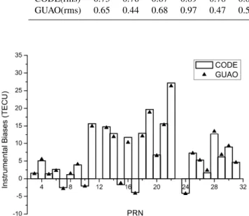
Fig. 1. Comparison of the instrumental biases issued by CODE with those estimated from GUAO data using the described method in 2004.
shell is divided into even meshes of 0.5 degrees by 0.1 h in latitude and local time, the ionospheric correlation region is limited to each little mesh area. The Eq. (7) is obtained only under the condition of the “conjunctions” occurring in the same mesh. So the function to weight the measurement con-tribution in different temporal and spatial scale over whole ionospheric shell used in the original SCORE method is not introduced here.
In this paper, for the convenience to analyze the influ-ence of the instrumental biases on the accuracy of iono-spheric TEC, the unit of instrumental bias is transferred as TECU, where 1 nanosecond (ns) is equivalent to 2.853 TECU (1 TECU = 1016/m2). Figure 1 shows the mean values of GPS satellite instrumental biases in 2004 estimated from GUAO observations using the method introduced above (relative to the instrumental bias of PRN 1). The results of instrumental biases issued by CODE are also shown in this figure, and the corresponding RMS of the biases in Fig. 1 is also given in Table 2. (The result of satellite PRN 2 and PRN 23 is not included due to significant satellite bias changes associated with equipment activation in 2004.) It can be seen that the accuracy of the two methods are very close.
3 Results and analysis
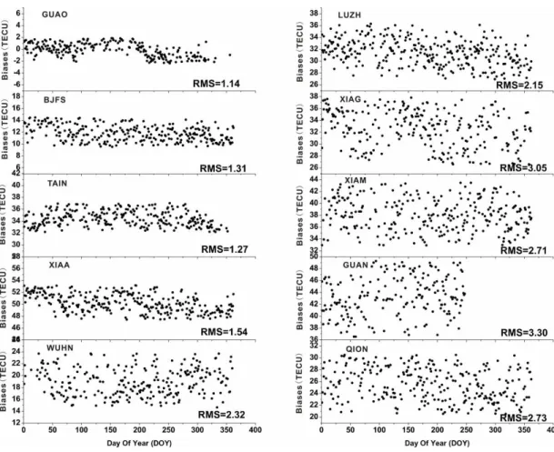
Figure 2 shows the instrumental biases of several GPS satel-lites estimated from the GUAO station in 2004 relative to the mean value of the whole year. The X-axis denotes the day of year (DOY). In order to compare the difference with the re-sults of the low latitude station clearly, the Y-axis range is set from−10 to 10 TECU for all listed satellites. For the PRN 19 satellite, there is a data gap before March 2004 due to the unavailability of the satellite. Figure 3 shows the satellites’ instrumental biases based on the data of the XIAM station relative to the mean value of the whole year in 2004. From Figs. 2 and 3, which are the results from the typical middle and low latitude stations, it can be seen that the instrumental biases estimated from the mid-latitude GUAO observations had small fluctuations throughout 2004, and nearly all of the instrumental biases appear in the range of−2∼2 TECU. The RMS values of instrumental biases throughout 2004 for all listed satellites are less than 1 TECU. Nevertheless, the satellite instrumental biases estimated from the XIAM ob-servations, which is located in the low latitude region, fluctu-ate much more extensively than that estimfluctu-ated from GUAO observations. The value between the maximum and mini-mum of instrumental biases for some satellites estimated from XIAM observations even reaches more than 15 TECU. In addition, the RMS values of the satellites for the whole year are obviously higher than the results estimated from the GUAO data, but usually less than 2.5 TECU.
Fig. 2.Satellite instrumental biases estimated from GPS data observed at GUAO station in 2004 (relative to the mean value).
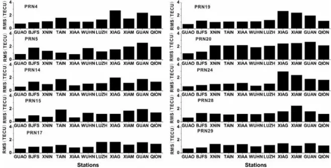
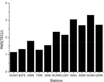
Fig. 4.RMS of instrumental biases of ten GPS satellites estimated from GPS data in 2004.
estimated from the GPS observations in 2004. From Fig. 4, it can be seen that, although there are a little exceptional sit-uations, the main tendency of the RMS value of the satellite instrumental bias is that the RMS values estimated from the data observed in the low latitude region is larger than that es-timated from the data in the middle latitude. The RMS value varies from approximately 1 to 3 TECU, but all RMS val-ues are less than 4 TECU. Furthermore, it can be seen that the RMS values of the satellite instrumental biases estimated from the QION station, located at the southern side of the equatorial anomaly north peak, are less than the RMS esti-mated from the XIAG, GUAN, and XIAM stations located just below the EIA crest. Certainly, the dependence of RMS on latitude does not show very obviously in the results es-timated from the data of these stations located in the tran-sitional region between middle and low latitude. The RMS of some satellites instrumental bias estimated from the BJFS and TAIN data seems larger than the other stations’. The data quality analysis using the occurrence of GPS cycle slip de-rived from the GPS data observed at two nearby sites reveals the existence of the data quality differences (Zhang et al., 2010). Even for the same type of the receiver and antenna, the so-called inter-individual differences of the observations exist due to the receivers’ hardware thermal noise conditions and GPS sites nearby environment. Although some measures are taken to alleviate the possible influence on the estimation of the GPS instrumental bias, the inter-individual differences of the receivers still exist. The larger RMS of the bias es-timated from BJFS and TIAN observation maybe illustrate that the inter-individual differences of the equipments and the observing environment can affect the accuracy of the bias es-timation. Even so, the main tendency of the latitude varying RMS is explicit in Fig. 4.
0 10 20 30 40 50 60
Latitude 40
60 80 100
TE
C
(TE
C
U
)
0.2 10.2
20.2
30.2
Fig. 5. The geographical latitudinal distribution (from 0◦N to 50◦N) of TEC along the 120◦meridional line calculated from IRI model (IRI model parameters: longitude: 120◦E; day of year: 280; local time: 12 LT; R12: 150; height range selection: 100–1000 km; height step: 1 km). The values labeled in the figure are the corre-sponding geomagnetic latitudes.
Other research has found that the distribution of the plas-maspheric electron content along the meridional line has a significant effect on TEC and GPS instrumental bias estima-tion, and the accuracy of the instrumental bias can be im-proved by properly considering the distribution of the plas-maspheric electron content (Lunt et al., 1999; Mazzella et al., 2002, 2007, 2009; Anghel et al., 2009; Carrano et al., 2009). Based on this improvement the distribution of the plasmas-pheric electron content was estimated using GPS measure-ments (Mazzella et al., 2002, 2007; Anghel et al., 2009; Car-rano et al., 2009). Besides the latitude-related distribution of the plasmasphere, the ionosphere also exhibits an obvi-ous latitude distribution near the EIA region (the geomag-netic latitude of peak EIA is about 10◦
−15◦
) that is mainly controlled by the ionospheric E region electric field (Kelley and Heelis, 1989). In Chinese longitudal sector, the influ-ence of the EIA can reach the region of the 40◦
N (about 30◦
Fig. 6.Receiver instrumental biases estimated from GPS data in 2004.
latitudinal distribution (from 0◦N to 50◦N) of the iono-spheric TEC along 120◦E meridional line obtained by in-tegrating ionospheric electron content from the height of 100 km to 1000 km that is calculated from International Ref-erence Ionosphere model (IRI) in solar maximum phase. The values labeled in the figure are the corresponding geomag-netic latitudes. The distribution of northern EIA can be seen obviously in this figure. With the latitude decreasing, the ionospheric spatial gradient in the meridian direction induced by the northern EIA increases gradually. It is observed that in solar maximum years, in the longitude sector of China in the latitude range from 30◦
N to 35◦
N, the gradient of iono-spheric TEC in the meridian direction induced by equato-rial anomaly reaches around 2 TECU/degree, and it becomes larger with latitude decreasing (Zhang et al., 2002). On the other hand, comparing with the mid-latitude ionosphere, the low latitude ionosphere exhibits more significant and com-plicated temporal variability due to the electro-dynamic pro-cess occurred in the ionospheric E and F region. Therefore, during the process of estimating instrumental bias, with the latitude decreasing, the error of the assumption, which the vertical ionospheric TECs at the different IPP but in a same divided mesh are equal (described in Eq. 7), becomes larger gradually due to significant spatial and temporal variations.
Fig. 7. RMS of the receivers’ instrumental biases estimated from GPS data in 2004.
this day are not given in this figure and the RMS value is calculated just based on the data before DOY 248. It can be seen in Fig. 6 that the scatter range of the instrumental bias estimated from the GPS data is different and the RMS value of the receiver instrumental bias located in mid-latitude is less than that in low latitude. In order to show this feature clearly, the RMS values of the receiver instrumental bias is given in Fig. 7 listed in the order of latitude. It can be seen that the RMS of instrumental bias increases with the latitude decreasing roughly, and the RMS value changes from about 1 TECU to 4 TECU.
The largest error source of the ionospheric TEC derived from GPS method can be the error of the measured or esti-mated instrumental bias. To a certain extent, the accuracy of the estimated instrumental bias determines the accuracy of TEC. From the RMS variation of the satellite and receiver instrumental bias corresponding to the latitudes mentioned above, it can be concluded that, besides the influence of the variability of the plasmasphere, the equatorial ionospheric anomaly that deviates the assumptions of ionospheric smooth variation and fixed ionospheric shell height also affect the ac-curacy of the bias estimation. The acac-curacy of TEC derived from stations located in the mid-latitude region is higher than that in low latitude. Considering the error of both GPS satel-lite and receiver instrumental biases based on the ionospheric model assumption, the accuracy of ionospheric absolute TEC derived from GPS data in the mid-latitude region using this method is around 2–4 TECU, whereas that in the low latitude region is around 6–8 TECU.
Besides the SCORE method, many advanced data-processing technologies and methods, such as neural net-works (Ma et al., 2005), Kalman filter (Sardon et al., 1994; Anghel et al., 2009; Carrano et al., 2009), SCORPION method that removes the contribution of the plasmasphere using some model (Mazzella et al., 2002, 2007), have been
used in the process to estimate the instrumental biases in the last decade. Nevertheless, no matter which methods are em-ployed, the condition of the temporal and spatial variation of the ionosphere has to be considered during the process to es-timate the GPS instrumental biases from raw GPS data, and the large horizontal gradient of the ionospheric TEC caused by the EIA certainly will affect the accuracy of the estimated bias. Although the receiver bias can be measured using some special equipments, such as GPS receiver calibrator (Dyrud et al., 2008), obtaining the instrumental bias independently of ionospheric condition is still impractical for most GPS users. Nevertheless, ionosphere exhibits temporal and spatial vari-ability, and up to now the accurate ionospheric model to de-scribe this variability is unobtainable. So, the influence of the ionospheric variability on the accuracy of the instrumen-tal bias estimation is difficult to remove completely. In the ionospheric morphological studies, the researchers should be aware of the errors. The advent of the GPS greatly stimulates the study of the ionospheric morphology and disturbance. Apart from traditional ionospheric study (Ho et al., 1996; Mendillo, 2006), the ionospheric disturbances related with some geo-related natural hazards, such as the great earth-quakes or severe meteorological disasters, also draw atten-tions from the global geophysicists (Liu et al., 2004; Wan et al., 1998; Xu et al., 2008). The spatial scale of the iono-spheric disturbances caused by these kinds of events gener-ally covers hundreds or thousands of kilometers, and the vari-ation of the ionospheric TEC disturbance is usually several TECU that is much less than that of the ionospheric storm. Therefore, during the process to derive the ionospheric TEC from the GPS data, the TEC error problem related to instru-mental bias should be noted. That is, attention should be paid to the results based on the ionospheric TEC derived from GPS data, and the reliability analysis is necessary for the study of the weak TEC disturbances that are less than or similar to the error scale of the TEC mentioned above.
4 Summary
With one bias estimation method, the instrumental biases es-timated from the GPS observations in the middle and low latitude region of Chinese longitude sector show obvious dif-ferences in the error scale. With the decrease in latitude, the spatial gradient of the ionosphere related to the ionospheric equatorial anomaly increase, and the RMS of the GPS in-strumental biases increase. Due to the lower spatial gradient and temporal variation in mid-latitude ionosphere, the satel-lite and receiver instrumental biases estimated using the same method are more accurate. The RMS values of the satel-lite instrumental bias estimated from GPS observations in 2004 are around 1 TECU, and the RMS values of the receiver instrumental bias is around 2 TECU in mid-latitude region. Nevertheless, the RMS values of GPS satellite instrumen-tal bias estimated from GPS observations in 2004 near the equatorial anomaly region are around 2 TECU, and those of receiver instrumental bias are 3–4 TECU.
Ionospheric TEC derived from GPS data has become one of the routine parameters to describe the ionospheric state in the past two decades. In the process of estimating iono-spheric TEC using GPS data, the main error is likely from the estimation of the instrumental bias, so the accuracy of the estimated instrumental bias will directly affect the ac-curacy of ionospheric TEC. From the analysis above, it can be concluded that the accuracy of the estimated instrumental bias are dependent on the validity of the assumption of the quiet and uniform ionospheric variation condition that must be confronted for any bias estimation methods. Furthermore, the RMS of instrumental bias can be used to estimate the ac-curacy of TEC based on the GPS method at different latitudes semi-quantitatively. For the estimation method used in this study, the estimated TEC error is around 2–4 TECU based on the mid-latitude GPS observations in 2004, and around 6–8 TECU based on the low latitude GPS observations at the same time.
In any study of the ionospheric morphology or the iono-spheric disturbance based on the GPS method, in partic-ular in the study of the weak temporal and spatial varia-tions (such as the ionospheric earthquake effect and the iono-spheric influence by meteorological process), the error anal-ysis is needed, to ensure the reliability of results based on ionospheric TEC.
Acknowledgements. We thank CMONOC and IGS for providing
highly precise GPS data. This work is jointly supported by the China NSFC (grants: 40674089, 40636032), China NRBRP (grant: 2006CB806306) and State Key Laboratory of Space Weather.
Topical Editor K. Kauristie thanks A. Mazzella and another anonymous referee for their help in evaluating this paper.
References
Anghel, A., Carrano, C., Komjathy, A., Astilean, A., and Letia, T.: Kalman filter-based algorithms for monitoring the ionosphere and plasmasphere with GPS in near-real time, J. Atmos. Sol.-Terr. Phy., 71, 158–174, 2009.
Brunini, C., Meza, A., and Bosch, W.: Temporal and spatial vari-ability of the bias between TOPEX- and GPS-derived total elec-tron content, J. Geodesy, 79, 175–188, doi:10.1007/s00190-005-0448-z, 2005.
Carrano, C. S., Anghel, A. F., Quinn, R. A., and Groves, K. M.: Kalman Filter Estimation of Plasmaspheric TEC using GPS, Ra-dio Sci., 44, RS0A10, doi:10.1029/2008RS004070, 2009 Ciraolo, L., Azpilicueta, F., Brunini, C., Meze, A., and Radicella,
S. M.: Calibration errors on experimental slant total electron content (TEC) determined with GPS, J. Geodesy, 81, 111–120, doi:10.1007/s00190-006-0093-1, 2007.
Coco, D. S., Coker, C., Dahlke, S. R., and Clynch, J. R.: Variability of GPS satellite differential group delay biases, IEEE T. Aero. Elec. Sys., 27, 931–938, 1991.
Dyrud, L., Jovancevic, A., Brown, A., Wilson, D., and Ganguly, S.: Ionospheric measurement with GPS: Receiver techniques and methods, Radio Sci., 43, RS6002, doi:10.1029/2007RS003770, 2008.
Ho, C. M., Mannucci, A. J., Lindqwister, U. J., Pi, X., Tsurutani, B., et al.: Global ionospheric perturbations monitored by the world-wide GPS network, Geophys. Res. Lett., 23, 3219–3222, 1996. Ho, C. M., Wilson, B. D., Mannucci, A. J., Lindqwister, U. J., and
Yuan, D. N.: A comparative study of ionospheric total electron content measurements using global ionospheric maps of GPS, TOPEX radar, and the Bent model, Radio Sci., 32, 1499–1521, 1997.
Kelley, M. C. and Heelis, R. A.: The Earth’s Ionosphere: Plasma Physics and Electrodynamics, Academic Press, 1989.
Lanyi, G. E. and Roth, T.: A comparison of mapped and measured total ionospheric electron content using Global Positioning Sys-tem and beacon satellites observations, Radio Sci., 23, 483–492, 1988.
Liu, J. Y., Chuo, Y. J., Shan, S. J., Tsai, Y. B., Chen, Y. I., Pulinets, S. A., and Yu, S. B.: Pre-earthquake ionospheric anomalies reg-istered by continuous GPS TEC measurements, Ann. Geophys., 22, 1585–1593, doi:10.5194/angeo-22-1585-2004, 2004. Lunt, N., Kersley, L., Bishop, G. J., Mazzella, A. J., and Bailey, G.
J.: The effect of the protonosphere on the estimation of GPS total electron content: Validation using model simulations, Radio Sci., 34(5), 1261–1271, 1999.
Ma, G. and Maruyama, T.: Derivation of TEC and estimation of instrumental biases from GEONET in Japan, Ann. Geophys., 21, 2083–2093, doi:10.5194/angeo-21-2083-2003, 2003.
Ma, X. F., Maruyama, T., Ma, G., and Takeda, T.: Deter-mination of GPS receiver differential biases by neural net-work parameter estimation method, Radio Sci., 40(1), RS1002, doi:10.1029/2004RS003072, 2005.
Mannucci, A. J., Wilson, B. D., Yuan, D. N., Ho, C. H., Lindqwis-ter, U. J., and Runge, T. F.: A global mapping technique for GPS-derived ionospheric total electron content measurements, Radio Sci., 33, 565–582, 1998.
7(6), 1092, doi:10.1029/2001RS002520, 2002.
Mazzella, A. J., Rao, G. S., Bailey, G. J., Bishop, G. J., and Tsai, L. C.: GPS Determinations of Plasmasphere TEC, Proceedings of the International Beacon Satellite Symposium 2007, edited by: Doherty, P., Boston College, USA, 2007
Mazzella Jr., A. J.: Plasmasphere effects for GPS TEC mea-surements in North America, Radio Sci., 44, RS5014, doi:10.1029/2009RS004186, 2009.
Mendillo, M.: Storms in the ionosphere: Patterns and processes for total electron content, Rev. Geophys., 44, RG4001, doi:10.1029/ 2005RG000193, 2006.
Niranjan, K., Srivani, B., Gopikrishna, S., and Rama Rao, P. V. S.: Spatial distribution of ionization in the equatorial and low-latitude ionosphere of the Indian sector and its effect on the pierce point altitude for GPS applications during low solar activity periods, J. Geophys. Res., 112(A5), A05304, doi:10.1029/2006JA011989, 2007.
Sardon, E., Rius, A., and Zarraoa, N.: Estimation of the transmit-ter and receiver differential biases and the ionospheric total elec-tron content from GPS observations, Radio Sci., 29(3), 577–586, 1994.
Sardon, E. and Zarraoa, N.: Estimation of total electron content using GPS data: How stable are the differential satellite and re-ceiver instrumental biases?, Radio Sci., 32, 1899–1910, 1997. Thampi, Smitha V., Balan, N., Ravindran, Sudha, Pant, Tarun
Ku-mar, Devasia, C. V., Sreelatha, P., Sridharan, R., and Bailey, G. J.: An additional layer in the low-latitude ionosphere in Indian longitudes: Total electron content observations and modeling, J. Geophys. Res., 112(A6), A06301, doi:10.1029/2006JA011974, 2007
Vladimer, J. A., Lee, M. C., Doherty, P. H., Decker, D. T., and Anderson, D. N.: Comparisons of TOPEX and Global Posi-tioning System total electron content measurements at equatorial anomaly latitudes, Radio Sci., 32, 2209–2220, 1997.
Wan, W., Yuan, H., Ning, B., Liang, J., and Ding, F.: Traveling ionospheric disturbances associated with the tropospheric vor-texes around Qinghai-Tibet Plateau, Geophys. Res. Lett., 25, 3775–3778, 1998.
Xu, G., Wan, W., She, C., and Du, L.: The relationship between ionospheric total electron content (TEC) over East Asia and the tropospheric circulation around the Qinghai-Tibet Plateau ob-tained with a partial correlation method, Adv. Space Res., 42, 219–223, 2008.
Zhang, D., Xiao, Z., Gu, S., Ye, Z., and Du, H.: The Study of ionospheric TEC during magnetic storm period on April 6∼8, 2000, Journal of Chinese Space Science, 22(3), 220–228, 2002. Zhang, D. H. and Xiao, Z.: Study of ionospheric response
to the 4B flare on 28 October 2003 using International GPS Service network data, J. Geophys. Res., 110, A03307, doi:1029/2004JA010738, 2005.
Zhang, D. H., Xiao, Z., Feng, M., Hao, Y. Q., Shi, L. Q., Yang, G. L., and Suo, Y. C.: The temporal dependence of GPS cycle slip related to ionospheric irregularities over China low latitude re-gion, Space Weather, 8, S04D08, doi:10.1029/2008SW000438, 2010.
Zhang, W., Zhang, D. H., and Xiao, Z.: The influence of geo-magnetic storms on the estimation of GPS instrumental biases, Ann. Geophys., 27, 1613–1623, doi:10.5194/angeo-27-1613-2009, 2009a