doi: 10.1590/0101-7438.2015.035.02.0285
PROJECT SCHEDULING OPTIMIZATION IN ELECTRICAL POWER UTILITIES
Cleber Mira
1*, Paulo R. Viadanna
1, Maria Ang´elica Souza
1, Arnaldo Moura
2,
Jo˜ao Meidanis
1,2, Gabriel A. Costa Lima
4and Renato P. Bossolan
3Received July 22, 2014 / Accepted May 2, 2015
ABSTRACT.The problem of choosing from a set of projects which ones should be executed and when they should start, depending on several restrictions involving project costs, risks, limited resources, depen-dencies among projects, and aiming at different, even conflicting, goals is known as the project portfolio selection (PPS) problem. We study a particular version of the PPS problem stemming from the operation of a real power generation company. It includes distinct categories of resources, intricate dependencies between projects, which are especially important for the management of power plants, and the preven-tion of risks. We present an algorithm based on the GRASP meta-heuristic for finding better results than manual solutions produced by specialists. The algorithm yielded solutions that decreased the risk by 47%, as measured by the company’s standard methodology.
Keywords: project portfolio management, power generation, optimization, scheduling.
1 INTRODUCTION
Decision makers are usually confronted with the problem of choosing the best portfolio of projects from a large set of available opportunities, according to a combination of criteria and a limited amount of resources over time. A project portfolio consists of a subset of the given projects, together with a schedule for their execution over a given period of time, and in such a way that all restrictions are obeyed. In this paper, we call this theproject portfolio selection
(PPS) problem. There are several formulations for the PPS problem [7] depending on specific constraints, objective functions, resource availability, labor policies, and timing assumptions. It may be possible to find many viable portfolios, but the main problem is to find one that is the best for a given set of conditions.
*Corresponding author.
1Scylla Informatics, Campinas, SP, Brazil. E-mails: [email protected]; [email protected] 2Institute of Computing, University of Campinas, Campinas, SP, Brazil.
3AES-Tietˆe, Bauru, SP, Brazil.
The single-objective function version of the PPS problem is a classical optimization problem [4, 2, 3, 21] with applications in finances [6], research and development [13, 22, 24], software devel-opment [18], and among many other fields. There is an extensive literature describing several ap-proaches to model PPS problem variants [11, 1]. Although not as studied as the single-objective function version, the multi-objective version of the PPS problem has gained increasing interest in recent years [7, 8, 12, 25, 27].
In [5] the authors propose a multi-step approach to what they name the portfolio management problem. The approach focuses on three main factors relevant to the portfolio problem: value maximization, risk minimization and strategic alignment. It also has a cross-listing of other works and a number of important portfolio management concepts they deal with.
A major Swiss utility is analyzed in [17]. Mean-variance portfolio theory is used to deal with current and possible future generation mixes in order to find efficient frontiers. A costs analy-sis is then performed taking into account physical boundaries in order to translate the obtained portfolio allocations into required installed capacities.
In [20], risk management is treated as an important and essential part in the decision making process used by power generation companies. The authors use both physical and financial trad-ing approaches to maximize profit potentials. Their methods take into consideration several risk factors, and are based on price risk and delivery risk. Bilateral contracts are formulated as general portfolio optimization problems with a risk-free asset andnrisky assets. Historical data from the electricity market is used to demonstrate the approach.
In the PhD Thesis [28], the author analyses investments into new electricity generating capacities under climate policy uncertainty, using conditional Value-at-Risk techniques. The investment problems are modeled as optimal portfolio selection problems. Differences between standard Markowitz portfolio frameworks and portfolio optimizations based on conditional Value-a-Risk are discussed, and results for real data are presented and compared.
Further discussion about other approaches to solving the single- and multi-objective versions of the PPS problem is also available [23].
Since our problem comes from a real case in the industry, with many specificities, none of the published approaches applies directly to it.
In Section 2 we outline the main characteristics of the particular PPS problem studied here. In Section 3 we present the problem input and describe the parameters needed to model and solve the problem. Section 4 describes the problem constraints. We discuss in Section 5 some optimization goals. Section 6 presents a heuristic to find good solutions for the variant of the PPS problem treated here. We show the results of experiments in Section 7, and summarize in Section 8.
2 Problem Description
2.1 Projects
A power generation company is periodically confronted with the selection and scheduling of projects that contribute to achieve diverse, usually conflicting, objectives such as:
1. Comply with government regulations;
2. Minimize risk exposures;
3. Increase return over investments;
4. Reduce operation costs;
In this power generation company, there are two kinds of projects:
1. Risk management projects: these projects are responsible for guarding against and mitigat-ing risks that might arise durmitigat-ing the power generation operation. They impact operational tasks, as well as other activities such as the refurbishing of installed equipment, the ac-quisition of new equipment, or the improvement of maintenance procedures. They can be scheduled with a certain amount of freedom, respecting a number of operational con-straints.
2. Non-risk management projects: these are projects that do not contribute to the preven-tion or mitigapreven-tion of risks. Examples are projects for the acquisipreven-tion of office supplies, of personnel safety equipment, or of employee uniforms, among others. Non-risk manage-ment projects also include projects that help the company reach its strategic goals,e.g., the construction of a new power plant, or projects that attend exclusively to regulatory de-mands, such as environmental legislation concerning reservoir area, production capacity, and power availability. Due to their nature, projects of this kind cannot be scheduled at will by the decision maker; they must follow a strict, predefined schedule.
The selected projects must be scheduled to start at specific months within a period of time called theplanning horizon(PH). The extent of the planning horizon, denoted byT, is typically 60 months in our case study. Non-risk management projects are consideredmandatory, that is, they must start at a prescribed initial month within the PH. Risk management projects are not manda-tory, which means that their specific characteristics – such as costs, risk guarding potential, and interdependencies – are scrutinized by a decision maker, who decides if, and when, to schedule them for execution.
2.2 Warning points
The generation of electricity is a complex process. As such, several undesired events might oc-cure.g., equipment failure, violation of government regulations, or accidents. Then, prevention against the occurrence of undesired events is a top priority and there is a consolidated process to achieve this control, consisting of the following steps:
1. Elicitwarning points, that is, identify specific conditions that may cause undesired events. Warning points are then used to guide specialists when they elaborate measures to prevent the occurrence of undesired events.
2. Assign to each warning point an amount of risk according to a standard set of criteria. Such criteria might include the probability of occurrence of their associated undesired events, how severe a safety hazard it can be, the severeness of occasional environment damages that might follow, or threats to the company image, among others. The amount of risk should be proportional to the impact the occurrence of the corresponding undesired events may cause, if the warning point is not controlled. Warning points are classified into two risk categories, namely,criticalandnon-critical. The non-critical category includes warning points with either a tolerable or moderate risk. The critical category includes warning points with an intolerable risk. The risk category is assigned by expert personnel and will be seen, in the sequel, to impact the scheduling of a project.
3. Devise projects thatcontrolthe warning points, in order to prevent or mitigate the impact of the associated undesired events. Usually, a warning point is controlled by agroup of projects. In our present modeling, all projects in a group are taken to contribute equally for controlling the risk associated to the warning point. According to the available data, and following field engineers advice, this was deemed reasonable in a first approach. Notice that a project may belong to more than one group of projects, and therefore it may contribute to control the risk of several warning points. The total risk controlled by a project is obtained by summing all the shares of risk the project controls in all groups it belongs to.
In this PPS problem variant we focus on controlling the risk assigned to warning points. The risk associated to a warning point can be considered completely averted only after all projects in its controlling group have been completely executed. Moreover, high-risk warning points must have their associated risk completely controlled by the end of a givendeadline, which is a specific month along the PH. Only high-risk warning points have an assigned deadline.
2.3 Power plants and generating units
Table 1– The list of symbols used throughout the text.
T size of planning horizon (PH) in months
I set of projects
[n] interval 1,2, . . . ,n
dp duration (in months) of projectp
IP set of projects in portfolioP
mp starting month of projectpin portfolioP
ep last month of execution of projectp
lp lead time of projectp
pm prescribed initial month for projectpin the manual solution
Gw group of projects controlling warning pointw
W set of all warning points
fw last month of the tardiest project controlling warning pointw
Dw deadline associated to high-risk warning pointw
Q the set{C AP E X,O P E X}
rp,m resource consumption of projectpin them-th month of its duration Pt,q set of projects of classqactive in montht
cP,t,q resource consumption of classqon monthtfor portfolioP CP,y,q yearly version ofcP,t,qabove
Sy,q resources available for classqand yeary
g(u,t) number of generating units halted at plantuon montht gL(u,t) same asg(u,t)but due to long-term projects
Rw risk of warning pointw
WP set of warning point effectively controlled by portfolioP
R(P) area under the risk curve for portfolioP VI set of viable portfolios for instanceI
Each power plant has a specific location associated to it. Besides their location, power plants are also associated to divisions, for management purposes. Both associations, into locations and divisions, have an influence on the operation of power plants. This influence will be reflected on the problem restrictions.
The PPS problem is a difficult problem [9] – NP-hard in the computer science jargon. Given its difficulty, we decided to approach this particular PPS problem using an heuristic of easy implementation and that provides good results.
3 PROBLEM INPUT
The input data provided by the company is composed by a set of projects, a set of warning points, a planning horizon, PH, the availability of resources along the PH, and other data about power plants and generating units.
The planning horizon is always taken to be five years, that is, its extentT is set to 60 months. However, the portfolio expected as a solution for the problem has anexecution horizon(EH) of ten years (2T): the first five years are the planning horizon, while the final five years serve to accommodate projects that, although initiated before the final month on the PH, will finish after the end of the PH. With a duplication of the PH period we can register how much a project that terminates beyond the last month in the PH will contribute to reduce the portfolio’s overall risk. Duplicating the planning horizon is enough, since no project execution is longer than five years.
3.1 Available resources
For administrative and fiscal reasons, and government regulations, resources must be classified into two categories: operational expenditures (OPEX) and capital expenditures (CAPEX). The costs of each project are always entirely of only one of these two categories.
Resource availabilities are presented in two series of five annual amounts. The first series des-ignates annual resource availabilities for CAPEX expenditures, and the second one represents annual values for OPEX expenditures. Annual resource availabilities for years after the PH are replicated from the given resource availability for the first five years, in both categories.
3.2 Projects
A project is defined by the following set of parameters and constraints:
1. Maintenance duration: for maintenance projects, this parameter indicates whether the project’s duration isshort-term(S) orlong-term (L). Fornon-maintenanceprojects, the indication is N.
2. Anarea: an identification of the administrative unit or power plant associated to a project. The administrative units include an “operation and management center” (COG), and an “information technology center” (IT). The power plants include: AGV, BAB, BAR, CAC, EUC, IBI, LMO, MOG, NAV, PRO, SJS, SJQ. See Table 2.
4. Halting start month: for a maintenance project, the halting start month indicates from which month, counting from its first execution month, the project will halt the correspond-ing generatcorrespond-ing unit.
5. Halting duration: for a maintenance project, the halting duration informs for how long, in months, the generating unit affected by the project will be halted.
6. A manually selectedinitial monthat which the project is scheduled to start. The set of all projects, together with the corresponding initial months, forms a portfolio, dubbed theinitial portfolio. This portfolio was manually constructed by expert engineers at the company, and can be used as a yardstick for comparison against other solutions.
7. A projectlead timeis the number of months, counting from the beginning of the PH, after which the project can be scheduled to start.
8. Aproject kind, which can berisk managementornon-risk management. The project kind is used to indicate whether a project is mandatory, and therefore must start at its assigned initial month. Non-risk management projects are mandatory.
9. Aresource classificationdesignating the kind of resource it consumes: OPEX or CAPEX. A project can consume resources from one category only.
10. A sequence of values, also referred to as the project’s costs, describing the amount of resources the project will consume in each month during its execution, starting with the initial month. Thedurationof a project is the number of months necessary for its execu-tion.
3.3 Warning points
Warning points are specified by the following parameters:
1. Anidentifier: a unique, numeric identifier.
2. Arisk measure: a rational number indicating the risk associated to the warning point.
3. Group of projects: a list of project identifiers that defines the group of projects that controls this warning point. Note that some projects may not belong to any group and, therefore, they do not contribute to risk control,e.g., a project for office supplies acquisition.
4. Arisk category: a qualitative classification of the risk into two categories: criticalor non-critical.
5. Adeadline: the latest month at which the warning point must be completely controlled. The deadline is present for high-risk warning points only.
3.4 Power plants and generating units
geographical locations and administrative divisions. Table 2 summarizes the administrative hi-erarchy of the company generation system, including the information about divisions, areas and power plants, geographical locations and the number of generating units in power plants.
The following parameters are provided for each power plant:
1. Plant identifier: a unique, three-letter code identifier;
2. Generating units: the number of generating units in the power plant;
3. Division: the division responsible for managing the plant;
4. Geographical location: the geographical location the plant resides in.
Table 2– Administrative hierarchy of the company system. The first column gives the administrative divi-sion the plant is subordinate to. The second column gives the area. The third column specifies the power plant location. The fourth column shows the number of generating units at the corresponding power plant.
Division Area/Plant Location Generating Units
COG COG – –
IT IT – –
AGV AGV AV 6
PRO NAV NAPI 3
PRO NAPI 3
BAR
BAB BBB 4
BAR BBB 3
IBI NAPI 3
LMO
CAC RP 2
EUC RP 4
LMO RP 2
MOG RMG 2
SJS RJM 2
SJQ RJM 1
4 CONSTRAINTS
In this section we list all constraints for this particular version of the PPS problem. Notice that this PPS version is not a linear problem as can be seen by the nature of its constraints like, for instance, the halting restriction expressed by Eq. (13). This does not pose a difficulty to our modeling, since we developed a variant of a GRASP meta-heuristic to solve the problem and, as is well known, a GRASP meta-heuristic can cope with nonlinearities.
will always assume thatT comprises an integral number of years, that is, it is a multiple of 12. For each projectp∈ I, we will indicate its duration, in months, bydp. For ease of reference, we
may write[n]for the interval[1,n], wherenis a positive integer. For a complete list of symbols used throughout the text, see Table 1.
A portfolio P is a set of pairs (p,m)where p is a project in I andm is the month in which project pis scheduled to start its execution, that is, P ⊆ I× [T]. We will indicate byIP ⊆ I
the set of projects present in portfolioP.
A portfolioPisvalidif it satisfies the following set of constraints.
Consistent scheduling. A project cannot be scheduled to start at two different months. If(p,m1)∈ Pand(p,m2)∈ Pthenm1=m2, for all p∈ IP. (1)
This means that a valid portfolioPis in fact a functionP:IP → [T]. From now on, we will let
mp=P(p)indicate the starting month andep=mp+dp−1 will be the last execution month
of projectp, whenp∈ IP.
Lead Time. A projectpcannot be scheduled to start before its lead timelphas passed. Then, mp>lp, for all p∈IP. (2)
Mandatory projects. A mandatory projectpshould always start at its prescribed initial month,
pm. Hence,
(p,pm)∈P, for all mandatory projectsp ∈I. (3)
Intolerable warning points. A warning point whose risk category is ranked as high-risk is an intolerable warning point and have a deadline associated to it. Each intolerable warning point must be completely controlled by the end of its deadline. This means that all projects in the control group of any intolerable warning point must be completed at that deadline LetGw ⊆ I
the group of projects controlling warning pointw. Recall thatW is the set of all warning points inI. Then we must have
Gw ⊆IP, for all intolerable warning pointsw∈W. (4)
This restriction being satisfied, define
fw = max
p∈Gw
mp+dp−1. (5)
We require, further, that
fw≤ Dw, for all intolerable warning pointsw∈W, (6)
whereDwstands for the deadline associated to an intolerable warning pointw.
Limited resources. Each project demands a certain amount of monthly resources from the month it starts until the last month of its execution. All resources consumed by a project are of the same kind as the resource classification associated to the project. The total yearly resource consumption of a certain kind, counting all projects that are under execution in that year, should not surpass the given amount of available resources of that kind and for that year.
The set of resource classifications isQ = {CAPEX,OPEX}. For any projectp ∈ I, letrp,m be
the resource consumption of project p during them-th month of its execution (1≤ m ≤ dp).
For a portfolioP, we collect in Pt,qthe set of all projects of classq ∈Qthat are active at month t ∈ [2T], that isPt,q= {p∈ IP|t∈ [mp,ep] }. Then
cP,t,q =
p∈Pt,q
rp,t−mp+1, t ∈ [2T],q ∈Q,Pa portfolio, (7)
gives the resource consumption at montht for all active projects of class q that are already scheduled at portfolioP. We can now collect the consumption of resources of a classqin a year
yfor a portfolioP:
CP,y,q =
t∈My
cP,t,q, y∈ [1,T/12],q∈ Q,
My= [12y−11,12y],Pa portfolio.
(8)
So, ifSy,qis the total amount of resources of classqavailable for yeary, this restriction imposes
the constraint
CP,y,q ≤Sy,q for ally∈ [1,T/12],q ∈ Q,Pa portfolio. (9)
We describe next the exclusion dependency constraints involving maintenance projects. We note that the only reason for halting a generating unit is the execution of a maintenance project that affects it. A maintenance project causes the halting of a generating unit for a limited period of time during its execution. That period is defined by the project’s halting start month and halting duration.
Halting restrictions by geographical location. Restrictions involving the halting of generat-ing units in some locations stem from engineergenerat-ing considerations. Letg(u,m)denote the number of generating units halted at plantu and monthmin a given portfolio, whilegL(u,m)denotes
the number of generating units halted at plantu and month m due to long-term maintenance projects. Referring to Table 2, the restrictions are as follows:
1. In the RP location, in any given month, if a plant has two or more generating units halted, the other plants cannot have any generating units halted. More formally, we have
g(u1,m)≥2→g(u2,m)=0, (10)
2. In the BBB location it must be observed that:
• In any given month, if a plant has two or more generating units halted, the other plants cannot have any generating units halted. Thus,
g(u1,m)≥2→g(u2,m)=0, (11)
form∈ [2T]andu1,u2∈ {B AB,B AR}, withu1=u2.
• In any given month, at most two generating units from the BAR plant can be down. Thus,
g(B AR,m)≤2, form∈ [2T]. (12)
• In any given month, two generating units from the BAB plant can be down simulta-neously, but only if none of the BAR plant generating units are halted. Thus,
g(B AB,m)=2
→
g(B AR,m)=0
, form∈ [2T]. (13)
3. In the NAPI location, at most two generating units can be down at any given month. Thus,
g(N AV,m)+g(P R O,m)+g(I B I,m)≤2, form∈ [2T]. (14)
4. In any given month, in the AV location, we can have at most two halted generating units due to long-term maintenance projects. Thus,
gL(AGV,m)≤2, form∈ [2T]. (15)
Halting restrictions at the AGV plant. In any given month, if two or more generating units from the AGV plant are down, then no generating unit from the BAB, NAV, or PRO plants can be halted, that is
g(AGV,m)≥2
→
g(B AB,m)
= g(N AV,m)=g(P R O,m)=0, m∈ [2T]. (16)
Halting restrictions by division. In any given month, no more than three generating units in the same division can be halted. Let Dbe the set of divisions in the company electric power generation system, as given by Table 2. For each divisiond ∈ D, letUd be the set of power plants ind. We must have
u∈Ud
g(u,m)≤3, form∈ [2T],d ∈D. (17)
In a practical scenario, real problems of this complexity might involve uncertainties, like a sched-uled project not terminating its execution or having its termination delayed due to unanticipated events [19, 14]. This is not the case with the present PPS problem, however. But it should be noted that the concept of risk, as managed by AES in this PPS problem, is not usual, as discussed in Subsection 2.1, and it is also not related to these kinds of uncertainties. Therefore, approaches that treat the more common kinds of uncertainty, as mentioned, are not directly applicable to this version of the PPS problem.
5 OBJECTIVE FUNCTION
A set of optimization goals can be proposed for the PPS problem depending on which aspect – costs, human resources, risks – one wants to focus upon. While planning and constructing a portfolio, the company decision makers focus their efforts on reducing the risk resulting from all uncontrolled warning points. For that, they try to judiciously select and schedule projects of the risk management kind. The objective function of the PPS problem studied here should also reflect the best choice of scheduling projects in order to guard against uncontrolled warning points. So, in this version of the PPS problem, we focused on the optimization goal ofreducing the risk of uncontrolled warning pointsin a portfolio.
As we advance through the EH time frame, projects terminate and warning points reach a con-trolled state. When that happens, the total stock of unguarded risks decreases until it reaches a minimum, ideally 0, at month 2T or earlier. The area under the risk curve summarizes in a single number two of the most relevant aspects of a portfolio: theamountof controlled risk and
whenthe risk is averted. That is, the earlier a warning point is effectively controlled, and the larger is the risk value associated to the warning point, the better is the corresponding portfolio. Therefore, we set the objective function to minimize the area under the risk curve associated to the portfolio.
Recall thatW is the set of all warning points in an input instanceI to the PPS problem. LetRw
denote the risk associated to warning pointw ∈ W. For a portfolioP we letWP ⊆ W be the set of warning points that are effectively controlled inP. Then, the area under the risk curve for
Pis
R(P)=2T
w∈W Rw−
w∈WP
Rw(2T − fw), (18)
where fw, given by Eq. (5), is the first month when warning pointw is finally controlled (see
Figure 1).
For a given input instanceI to the PPS problem, letVIbe the set of all viable portfolios that can
be obtained from I. The goal, then, is to construct a portfolioP⋆such that R(P⋆)is minimum among{R(P)|P ∈ VI}. In the next section we describe a heuristic strategy that searches for
g
2TwRw
Time 2T
W8
2T−fw fw
(2T−fw)Rw W7
W6
W5
W4
W3
W2
W1
Rw
R(P) T
Risk
Figure 1– Illustration of the area under the risk curve.
6 A GRASP VARIANT FOR THE PPS PROBLEM
We describe a variant of the GRASP meta-heuristic for finding solutions for the PPS problem treated here. Those solutions will prove to be better than the manually produced solutions pro-vided by specialists. GRASP is a multi-start meta-heuristic that generates good quality solutions for many combinatorial optimization problems [26, 10], besides being of fast implementation, being easily comprehensible, and not requiring restrictive assumptions of mathematical opti-mization models; e.g. linear constraints. Thus, the GRASP meta-heuristic is suitable as a first approach to try and find better solutions than the manual ones. The differences between our GRASP variant and the original meta-heuristic are explained as follows.
The algorithm repeats two phases:
(i) A construction phase in which a feasible solution is obtained; and
(ii) a local search phase in which the algorithm finds a local optimal solution by iteratively checking whether there is a better solution in a neighborhood of the current solution.
The pseudo-code for the GRASP routine is presented as Algorithm 1. In the next two subsections the construction and local search phases are discussed more fully. The choices of parameters appearing in the algorithms are discussed in more detail in Section 7.
Algorithm 1GRASP-based routine for the PPS problem
1. Initialize an empty portfolio as the current BEST SOLUTION. 2. forRiterationsdo
3. // Construction phase
4. Initialize an empty pool of solutions. 5. while||<Cdo
6. Construction procedure returns a solutionPfor the PPS problem. 7. ifPsatisfies the intolerable warning point constraintthen
8. IncludePinto the poolof solutions.
9. end if
10. end while
11. // Local search phase
12. forEach solutionPin the firstβbest solutions indo
13. Let P = LOCAL SEARCH(P)
14. ifP is better than BEST SOLUTIONthen
15. BEST SOLUTION = P
16. end if
17. end for
18. end for
19. return BEST SOLUTION.
6.1 The Construction Phase
The first phase in our GRASP-based algorithm consists in the repeated execution of a construc-tion procedure. As shown in Algorithm 1, the construcconstruc-tion procedure produces a soluconstruc-tion and checks whether it satisfies the intolerable warning point constraint as expressed by Eqs. (4) and (6). These constraints require that all projects that control warning points must be scheduled in such a way that the corresponding warning points are totally under control before their deadlines are reached. If the portfolio is valid, then it is included in the pool of constructed solutions; otherwise, it is discarded. Feasible solutions are inserted into the pool until its capacityC is reached. Notice that the same solution might be included into the pool more than once. This does not seem to be a problem, however, and, moreover, since the solutions are relatively large structures, checking for equality is costly and does not seem to be worth the effort. The bestβof the constructed solutions in the pool are chosen as input solutions for the local search phase.
Two kinds of construction procedures were considered: an adaptive one and a non-adaptive one. We start with the non-adaptive procedure.
6.1.1 The non-adaptive procedure
The non-adaptive heuristic was devised as a simple procedure using two candidate lists of pairs
(p,m)of projectsp ∈IP and potential starting monthsm∈ [lp+1,min(M Dw−dp+1,T)],
whereM Dwis the minimum among all deadlines associated to all intolerable warning pointsp
parameter associated to a pair(p,m)should measure the gains obtained by scheduling projectp
at monthm, based not only on p’s ability to control risk, but also on its total cost. Notice that a project with a large value of controlled risk may be less cost-effective in terms of controlled risk per unit of cost than another project [23]. Notice also that we use two candidate lists instead of a single list, as is standard in the construction phase of a GRASP routine. This allowed us to classify the projects into two priority categories.
LetI be the set of projects in an input instance for the PPS problem, with planning horizonT, and warning point setW. In order to assess the cost-effectiveness of a pair(p,m) ∈ I × [T], we computebp,m, thebenefitof the pair(p,m). Let Rpbe the sum of warning point risk shares
projectpcontributes to control, computed over all warning points inW, and recall thatrp,tgives
the resource consumption of projectpduring itst-th month of execution. We let
bp,m=Rp
(2T −m−dp+1)/ dp
t=1 rp,t
, (19)
so thatbp,mexpresses the amount of risk project phelps to control, weighted by how long that
contribution is effective per unit of cost.
The portfolio construction procedure initially pre-processes the input data to schedule all manda-tory projects inI, which are then removed from I. Next, all pairs(p,m)∈ I × [T], have their benefit calculated, and the two candidate pair lists are built and sorted in non-increasing order of benefit. Thehigh-risk sorted pairs(HRSP) list involves pairs(p,m)where projectpcontributes to control high-risk warning points. Thesorted pairs(SP) list involves all the remaining pairs in I × [T]. We split the standard GRASP candidate list in two parts in order to give pairs in the HRSP list a higher priority over the SP list, since the corresponding projects help control high-risk warning points.
The algorithm proceeds to construct a portfolio by iteratively choosing a pair(p,m)from one of the two candidate lists. The next pair is chosen from the HRSP or the SP lists with probabilities
ηand 1−η, respectively. Once the list to choose the next pair from is determined, the next pair
(p,m)is randomly chosen from among the firstkpairs in that list. Then pair(p,m)is included in the portfolio being constructed if, by including it, the new portfolio does not violate any of the followinglocal constraints:
• “consistent scheduling”, Eq. (1);
• “lead time”, Eq. (2);
• “limited resources per year”, Eq. (9); and
• “halting restrictions”, Eqs. (10–17).
Observe that, at each iteration, as a new pair(p,m)is included, the available resources for each year decrease, reflecting the resource usage of project p, and the cycle repeats until no pair
(p,m)can be included in the portfolio.
We summarize the non-adaptive procedure used in the construction phase as Algorithm 2.
Algorithm 2Non adaptive construction procedure for the PPS problem
1. InitializePas an empty portfolio. 2. for allmandatory projectsdo
3. Schedule each mandatory project at its initial scheduled month. 4. Subtract mandatory project’s resources from the available resources. 5. end for
6. Calculate the riskRpof each remaining projectp.
7. Construct the HighRiskSortedPairs (HRSP) list of high risk project×month pairs, sorted by benefit value.
8. Construct the SortedPairs (SP) list of remaining project×month pairs, sorted by benefit value. 9. whileHRSP is not empty or SP is not emptydo
10. If one of the lists is empty, choose the other one, otherwise, randomly choose between HRSP and SP with probabilitiesηand 1−η, respectively.
11. Get a pair(p,m)randomly chosen from the firstkpairs at the top of the chosen list. 12. Remove pair(p,m)from the chosen list.
13. if(pis not already scheduled)and(adding(p,m)to the solution does not violate local constraints)
then
14. LetP=P∪ {(p,m)}. 15. else
16. Discard pair(p,m). 17. end if
18. end while
19. // Any remaining projects in SP and HRSP are not scheduled. 20. ReturnP.
6.1.2 The adaptive procedure
An adaptive version of the construction procedure involves the recalculation of the benefits of each remaining pairs in the candidate lists, after a new pair is included in the portfolio being constructed. After recalculation, the lists are sorted again.
The benefit function given by Eq. (19) is a first attempt to express the cost-effectiveness of scheduling a project at a certain month. However Eq. (19) does not take into account the im-pact on available resources caused by scheduling a new project. Given a portfolioP, we want to measure the impact of including a new pair(p,m)in Pby estimating which fraction of the presently available resources a new pair(p,m)will consume, at each month project pis in exe-cution. Furthermore, since costs are grouped annually, we need to sum p’s resource consumption over all months it is active in each year.
We denote byM(p,m,y)the set of months project pwill be active during yeary, if it starts at monthm. Note that, in this case, pwould end its execution at monthep =m+dp−1. Note
also that 12(y−1)+1 is the first month of yeary, and 12yis its last month. We then have, for
y∈ [1,2T/12]:
M(p,m,y)=
⎧ ⎪ ⎪ ⎨
⎪ ⎪ ⎩
∅, if 12y<morep<12(y−1)
[m,min{ep,12y}], if 12(y−1) <m≤12y
Algorithm 3Adaptive construction procedure for the PPS problem
1. InitializePas an empty portfolio. 2. for allmandatory projectsdo
3. Schedule each mandatory project at its initial scheduled month. 4. Subtract mandatory project’s resources from the available resources. 5. end for
6. Calculate the riskRpof each remaining projectp.
7. Construct the HighRiskSortedPairs (HRSP) list of high risk project×month pairs, sorted by adaptive benefit.
8. Construct the SortedPairs (SP) list of remaining project×month pairs, sorted by adaptive benefit. 9. whileHRSP is not empty or SP is not emptydo
10. If one of the lists is empty, choose the other one, otherwise, randomly choose between HRSP and SP with probabilitiesηand 1−η, respectively.
11. Get a pair(p,m)randomly chosen from the firstkpairs at the top of the chosen list. 12. Remove pair(p,m)from the chosen list.
13. if(pis not already scheduled)and(adding(p,m)to the solution does not violate local constraints)
then
14. LetP=P∪ {(p,m)}. 15. else
16. Discard pair(p,m). 17. end if
18. Recalculate the adaptive benefit of each remaining pair in SP and HRSP. 19. Reorder SP and HRSP lists according to the new adaptive benefit values. 20. end while
21. // Any remaining projects in SP and HRSP are not scheduled. 22. ReturnP.
Then, ifh(p,m,y)gives the resource consumption of project p during year ywhen started at monthm, we have
h(p,m,y)=
⎧ ⎪ ⎨
⎪ ⎩
0, ifM(p,m,y)= ∅
j∈M(p,m,y)
rp,j−m+1, otherwise. (21)
Recall that, by Eq. (8),CP,y,q gives the total resource consumption for projects of categoryqin
a portfolioP during yeary, and Sy,q is the total amount of resources of categoryq in a yeary,
as given by the input instance. Then,
κ(p,m,y)= h(p,m,y) Sy,q−CP,y,q
, (22)
gives the fraction of the currently available resources, at year y, that will be consumed by the inclusion of a pair(p,m)in the current portfolioP, whereq is p’s category. To avoid division by zero, whenSy,q=CP,y,q, we setκ(p,m,y)=0.
The maximum fraction of yearly resource usage that a project pwill incur when the pair(p,m)
is considered for inclusion in a portfolioPis, then,
ρ(p,m)= max
1≤y≤T/12κ(
p,m,y). (23)
In order to recalculate the cost-effectiveness of a project p being scheduled at monthm in a portfolioP, and now taking into consideration the changes in available resources, we adopted as a measure of its effectiveness its adaptive benefitba(P,p,m), defined as
ba(P,p,m)=Rp
(2T −m−dp+1)/ρ(p,m)
. (24)
We note that every project consumes a non-null amount of resources in its corresponding cate-gory. The adaptive construction procedure is shown in Algorithm 3.
6.1.3 Comparing the construction strategies
We performed some experiments in order to compare the adaptive and the non-adaptive construc-tion procedures. We used as input instance the real-world based data described in Secconstruc-tion 7.
In order to check how much the resource usage has an impact on the quality of solutions, we performed experiments using variations on the adaptive benefitρ(p,m)described by Eq. (23), namely, we used the minimum, the average and the sum of the fractions of resource usages. We also used a pool with a capacityC of 100 solutions and also recorded the number of unfeasible solutions obtained until we reached full capacity. Table 3 shows the result of these experiments, where the real instance was used as input to the algorithm. The first column defines the con-struction strategy, the second column specifies how the fraction of yearly resource consumptions are combined, the next two columns give the best and the average values of the optimized objec-tive function (OOF) values, respecobjec-tively, the last two columns report the number of unfeasible solutions that were constructed and the running times, respectively.
Table 3– Construction strategy, best solution, average solution value (both in 106risk-month units), number of solutions, running time values (in seconds) for a real-world input instance.
Strategy resource usage best OOF avg OOF unfeasible solutions Time (s)
Non adaptive 0.570 0.638 0 74
Adaptive
avg 0.645 0.698 118 2343
max 0.741 0.846 43 1417
min 0.739 0.820 24 932
sum 0.649 0.700 128 1691
From Table 3, we find that the best solution found by the adaptive procedure – using the max-imum resource usage in the benefit function – is around 23.4% worse than the one found by the non-adaptive procedure. In addition, the adaptive procedure finds more invalid solutions and takes considerably more time to be executed than the non-adaptive strategy. Given these limita-tions on the side of the adaptive procedure, we decided to adopt the non-adaptive procedure in our GRASP-based heuristic.
6.2 Local search
executed. The local search starts at the input solution and examines its neighborhood, checking whether there is a better solution in terms of the objective function, using a best improvement strategy. It iteratively repeats the search in the neighborhood of each new solution until no better solution is found. The best solution thus found is then returned. The local search procedure is shown as Algorithm 4.
Algorithm 4Local search procedure
1. LetPbe the initial solution. 2. repeat
3. Get the list of neighborsNof the current solutionP. 4. Search throughN, using a best improvement strategy. 5. ifan improved solutionQwas foundthen
6. LetP= Q 7. end if
8. untilThere is no improved solution for the current solutionP. 9. return Portfolio P.
A fundamental aspect of a local search procedure concerns how the neighborhood of a solution is defined. We defined the neighborhood of a portfolio as the set of portfolios where each neighbor is obtained by re-scheduling one of its projects. If a project was originally scheduled at monthm, a neighbor is obtained by re-scheduling it at months fromm−tom+, avoiding the currentm, and whereis a fixed parameter. If re-scheduling leads to infeasibility, or to a project starting at a month beyondT, that neighbor is discarded. We note also that only projects whose start times are in the interval[1,T]are considered for re-scheduling. Another relevant aspect of the local search is how the neighborhood is searched. We implemented a best improvement strategy, which searches through all projects in the neighborhood and selects the best one. Algorithm 5 shows the procedure to construct the neighborhood of a portfolio.
Algorithm 5Returns the neighborhood of a solution
1. LetPbe the initial solution.
2. Initialize an empty list of solutionsN. 3. for all pairs(p,m)inPdo
4. for allmonthstin the interval
m−,m+
− {m}do
5. Q=P− {(p,m)}∪ {(p,t)}
6. ifQis feasiblethen
7. LetN=N∪ {Q}
8. end if
9. end for
10. end for
11. return List of neighbors N
7 EXPERIMENTS
In the company input instance, we had 1411 projects for a planning horizon comprising the years 2013–2017. The total number of warning points were 434 and the sum of all attributed risk values was around 25×103risk-units. Risk values were measured in a relative, dimensionless, number of “risk points”. The annual costs were 1.5, 1.0, 1.7, 1.3, and 0.7, expressed in 109monetary units, the Brazilian real. These figures all stemmed from real values, but they were multiplied by an undisclosed constant, in order to comply with the company confidentiality policies which do not permit the real values to be disclosed in a text that is publicly accessible.
The amount of available yearly CAPEX resources was obtained by summing up the CAPEX costs of all projects in the initial manual solution that were active at each year. Yearly OPEX available resources were obtained in a similar fashion.
7.1 Input instances
In order to assess the indicator values and test the robustness of the heuristic, we compared the manual portfolio solution for a real-world instance against the solution generated by the algorithm for that same instance. The manual portfolio solution was built by expert managers and engineers at the company.
In order to assess the robustness of the procedure, we used the real-world instance provided by the company as a seed for generating similar instances, and randomly disturbed the seed instance data, in a controlled way and by small margins. The disturbance procedure applied the following modifications to the real instance data, wheredwas a fixed disturbance factor:
Project costs: modified byx%, withxrandomly chosen between−d and+d.
Warning point risks: modified byx%, withxrandomly chosen between−dand+d.
Other parameters: not modified in the disturbed instances.
Using these modifications, we generated 10 instances for a 5% disturbance factor. We decided to adopt the disturbance factor of 5% because, according to engineers, modifications in the overall cost beyond 5% in a year are unlikely in a traditional industry such as in the electrical power generation industry, whose assets do not change by a large amount yearly.
7.2 Heuristic parameters
Before running the robustness experiment, we performed some calibration in order to identify adequate values for some of the GRASP parameters.
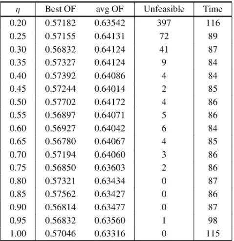
Table 4– Probability of choosing HRSP list (η), best and average solution values (OF, for objective function; in 106risk-month units), number of un-feasible solutions (Unun-feasible), and running time values (Time) in seconds.
η Best OF avg OF Unfeasible Time 0.20 0.57182 0.63542 397 116 0.25 0.57155 0.64131 72 89 0.30 0.56832 0.64124 41 87
0.35 0.57327 0.64124 9 84
0.40 0.57392 0.64086 4 84
0.45 0.57244 0.64014 2 85
0.50 0.57702 0.64172 4 86
0.55 0.56897 0.64071 5 86
0.60 0.56927 0.64042 6 84
0.65 0.56780 0.64067 4 85
0.70 0.57194 0.64060 3 86
0.75 0.56850 0.63603 2 86
0.80 0.57321 0.63434 0 87
0.85 0.57562 0.63427 0 86
0.90 0.56814 0.63477 0 87
0.95 0.56832 0.63560 1 98
1.00 0.57046 0.63316 0 115
average solution values, as well as gives rise to few unfeasible solutions and shows good running time figures. This choice increases the odds that a high-risk controlling project will be scheduled earlier in the portfolio.
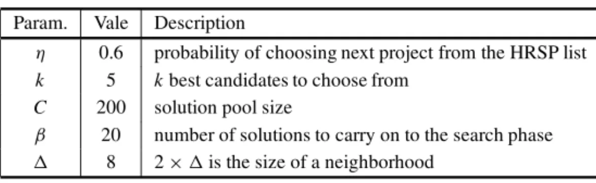
While the construction procedure was producing a new portfolio, the next project and month pair,(p,m), to be inserted in the current partial solution was randomly chosen among the first
k best candidates in the sorted candidate list. We set k equal to 5, because this value was a good compromise between enforcing the randomized aspect of the heuristic while not loosing the greedy advantage of having the candidate list sorted.
We performed several experiments (results not shown) to decide on the best values for parameters
C, the solution pool size, andβ, the number of solutions to carry on to the search phase. Since the local search phase is the most time consuming computation performed by the heuristic, it proved to be an advantage to useβ < C. The experiments took as input the real instance, as well as the disturbed instances described in Section 7.1. We finally decided on 200 for the pool capacityCand setβto be 10% of the capacity.
For the local search phase, we experimented with distinct values for the parameter, used in finding neighbor solutions. We found empirically that settingto 8 covers a good amount of neighbor solutions without compromising the algorithm’s performance.
Table 5– GRASP parameters values.
Param. Vale Description
η 0.6 probability of choosing next project from the HRSP list k 5 kbest candidates to choose from
C 200 solution pool size
β 20 number of solutions to carry on to the search phase
8 2×is the size of a neighborhood
7.3 Results and analysis
The GRASP based heuristic was executed once for each input instance, and the best solution was retained. The experiments were performed in an IntelR i3 Dual CoreR HT 1333GHz CPU, with
4Gb of RAM, running the Ubuntu GNU/Linux distribution, version 12.04 LTS, with kernel 3.5.0. The algorithm was implemented using the GO 1.1.2 programming language for its enhanced performance and ease of coding. In order to improve the algorithm’s performance, both the construction and local search procedures were implemented using GO parallel programming features.
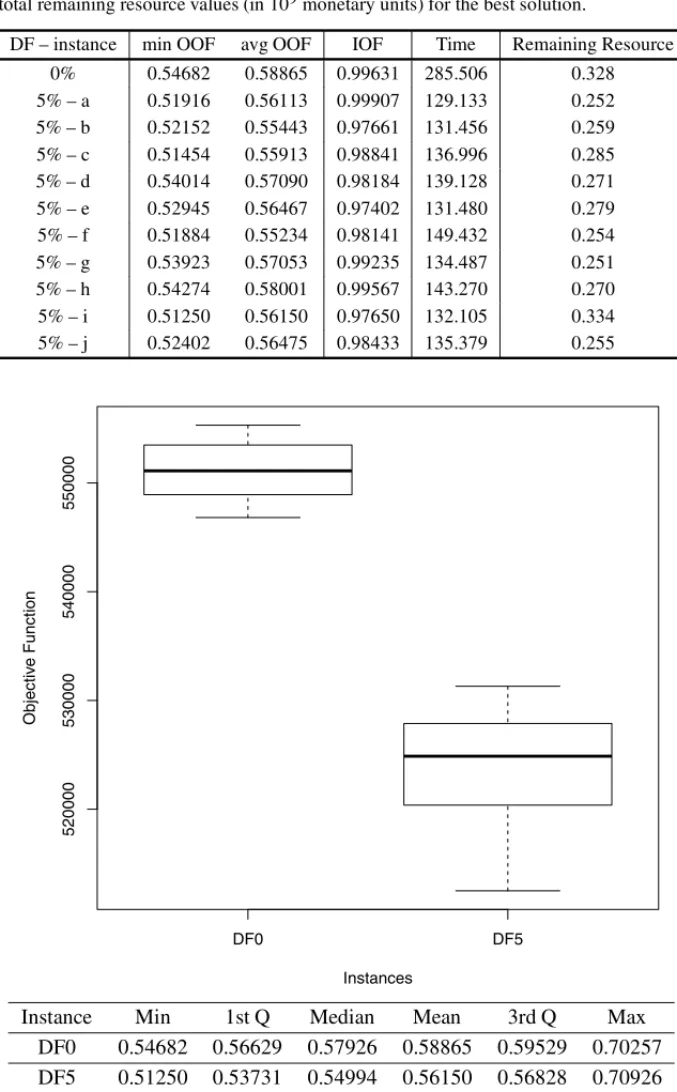
The results are summarized in Table 6. The first column shows the disturbance factor (DF) and an instance identification. A DF of 0% refers to the real instance. The second and third columns are, respectively, the best and the average optimized objective function (OOF) values in risk-month units, where a risk-month unit is, of course, one month times one risk-unit. The next column gives the objective function value for the corresponding manual portfolios (IOF) in risk-month units. The next to last column informs the total running time (Time) for executing one run for each instance, in seconds, and the last column (Remaining Resource) gives the total remaining resource values (in 109monetary units) when the best portfolio found adopted as a solution for the PPS.
Besides the objective function value, we also obtained the total amount of remaining resources after each portfolio was constructed, in order to check the impact of the heuristic on resource consumption. Table 6 contains a summary of the total remaining resources (in 109monetary units) along all the PH, and per input instance. The first line corresponds to the undisturbed in-stance, and each of the subsequent lines gives the result for the corresponding disturbed inin-stance, as described in Section 7.1.
The results show that the heuristic consistently found solutions whose objective function values were around 47% better when compared to the corresponding values for the manual, undisturbed solutions. This behavior was repeated when the algorithm took as input any of the disturbed instances, attesting to its robustness when relatively small changes were applied to the real input instance.
Table 6– Best, average, and input instance solution values (in 106risk-month units), and running time values (in seconds) for distinct input instances. The last column contains total remaining resource values (in 109monetary units) for the best solution.
DF – instance min OOF avg OOF IOF Time Remaining Resource
0% 0.54682 0.58865 0.99631 285.506 0.328 5% – a 0.51916 0.56113 0.99907 129.133 0.252 5% – b 0.52152 0.55443 0.97661 131.456 0.259 5% – c 0.51454 0.55913 0.98841 136.996 0.285 5% – d 0.54014 0.57090 0.98184 139.128 0.271 5% – e 0.52945 0.56467 0.97402 131.480 0.279 5% – f 0.51884 0.55234 0.98141 149.432 0.254 5% – g 0.53923 0.57053 0.99235 134.487 0.251 5% – h 0.54274 0.58001 0.99567 143.270 0.270 5% – i 0.51250 0.56150 0.97650 132.105 0.334 5% – j 0.52402 0.56475 0.98433 135.379 0.255
DF0 DF5
520000
530000
540000
550000
Instances
Objectiv
e Function
Instance Min 1st Q Median Mean 3rd Q Max DF0 0.54682 0.56629 0.57926 0.58865 0.59529 0.70257 DF5 0.51250 0.53731 0.54994 0.56150 0.56828 0.70926
8 CONCLUSIONS
We modeled a project portfolio selection (PPS) problem derived from a large electrical power generation and distribution company, operating in Brazil. Besides traditional obstacles, such as resource constraints, the problem also involves complex features, such as elaborate exclusion dependencies among projects and an intricate relationship among projects that control warning points.
We proposed a variant of the GRASP meta-heuristic for solving this specific PPS problem. We modified the construction phase by using a greedy randomized procedure to construct feasible solutions that are stored in a pool of solutions, instead of the standard practice of constructing a single solution from a single candidate list. Firstly, the greedy procedure used two candidate lists to distinguish high-risk versus low-risk projects. Secondly, only a fraction of the best solutions in the pool are fed into the local search phase, which uses a best improvement strategy. Neighbor solutions used in the local search procedure are defined by changing a project’s scheduled time by a small amount.
While designing the heuristics, we were not sure about which one of the two construction strate-gies, namely adaptive or non-adaptive, would provide better solutions. Therefore, we experi-mentally evaluated their performance and the quality of their solutions using a real-world input instance. It turned out that the non-adaptive strategy produced better solutions within a smaller running time, even when we adopted different adaptive benefit functions. In this particular exper-iment, the average value from all solutions produced by the non-adaptive strategy were nearer to the overall best solution values than any best solution produced by any of the adaptive procedures tested.
We performed experiments using real-world input instances in order to find appropriate parame-ters for the heuristics and to assess the algorithm robustness. The heuristics showed a significant improvement, up to around 47%, over the manual solutions when treating instances of real data, as well as when taking disturbed data as input. We note that when creating these manual solu-tions, company experts were, likewise the optimization routine, mainly concerned with control-ling the risks as soon as possible, so that comparing both solutions, at this stage, was meaningful and fair.
As for future work we can envisage the inclusion of new constraints concerning different cate-gories of available resources, such as human resources, the concurrent use of multiple objective functions, and versions of the problem where projects can be made available, or be dismissed, in a dynamic fashion. That is, given an optimized portfolioP, after the company started executing the projects scheduled as indicated in P, some urgent new projects might arrive which would have to be inserted in P, maybe dropping other projects that did not yet started. It would be interesting to have a, maybe lighter, algorithm that could modify P accordingly. In a similar fashion, projects in P that did not yet started could be deemed as no longer necessary and, in this case, such projects could be dropped from P, maybe making room to accommodate in P
ACKNOWLEDGMENTS
The authors would like to thank the company for their technical support and real data sets, and thank the National Agency for Electrical Energy (ANEEL) for their financial support (grant PD 0064-1021/2010).
REFERENCES
[1] ANANDALINGAMG & OLSSONC. 1989. A multi-stage multi-attribute decision model for project selection.European Journal of Operational Research,43(3): 271–283.
[2] ARCHERN & GHASEMZADEHF. 1998. A decision support system for project portfolio selection. International Journal of Technology Management,16(1): 105–114.
[3] ARCHERN & GHASEMZADEHF. 1999. An integrated framework for project portfolio selection. International Journal of Project Management,17(4): 207–216.
[4] BAKERN & FREELANDJ. 1975. Recent advances in R&D benefit measurement and project selection methods.Management Science,21(10): 1164–1175.
[5] BENAIJAK & KJIRIL. 2015. Project portfolio selection: Multi-criteria analysis and interactions between projects. CoRR, abs/1503.05366.
[6] CAMPBELLJ & CAMPBELLR. 2001. Analyzing and managing risky investments. Corporate Pub-lishing International, Grosvenor Business Tower, Office 804, Dubai 13700, United Arab Emirates. 1st edition, ISBN-13: 978-0970960702.
[7] CARAZOA, G ´OMEZT, MOLINAJ, HERNANDEZ´ -D´IAZA, GUERREROF & CABALLEROR. 2010. Solving a comprehensive model for multiobjective project portfolio selection.Computers & Opera-tions Research,37(4): 630–639.
[8] CHIAMS, TANK & ALMAMUMA. 2008. Evolutionary multi-objective portfolio optimization in practical context.International Journal of Automation and Computing,5(1): 67–80.
[9] DOERNERK, GUTJAHRW, HARTLR, STRAUSSC & STUMMERC. 2004. Pareto ant colony opti-mization: A metaheuristic approach to multiobjective portfolio selection.Annals of Operations Re-search,131(1): 79–99.
[10] FESTAP & RESENDEM. 2011. GRASP: basic components and enhancements.Telecommunication Systems,46(3): 253–271.
[11] FOXG, BAKERN & BRYANTJ. 1984. Economic models for R and D project selection in the pres-ence of project interactions.Management Science,30(7): 890–902.
[12] GUTJAHRW, KATZENSTEINERS, REITERP, STUMMERC & DENKM. 2010. Multi-objective de-cision analysis for competence-oriented project portfolio selection.European Journal of Operational Research,205(3): 670–679.
[13] HENRIKSENA & TRAYNORA. 1999. A practical R&D project-selection scoring tool.Engineering Management, IEEE Transactions on,46(2): 158–170.
[15] ISO 2009a.ISO GUIDE 31000:2009 “Risk management – Principles and guidelines”. International Standards Organization, Chemin de Blandonnet 8, CP 401, 1214 Vernier, Geneva, Switzerland. Pre-pared by IEC Technical Committee 56 – ‘Dependability’, and the ISO Technical Management Board’s Risk Management Working Group.
[16] ISO 2009b.ISO GUIDE 73:2009 “Risk Management – Vocabulary”. International Standards Orga-nization, Chemin de Blandonnet 8, CP 401, 1214 Vernier, Geneva, Switzerland. Prepared by the ISO Technical Management Board Working Group on Risk Management.
[17] KIENZLE F, KOEPPELG, STRICKER P & ANDERSSONG. 2007. Efficient electricity production portfolios taking into account physical boundaries. InProceedings of the 27th USAEE/IAEE North American Conference.
[18] LEEJ & KIM S. 2000. Using analytic network process and goal programming for interdependent information system project selection.Computers & Operations Research,27(4): 367–382.
[19] LIESIO¨ J, MILDP & SALOA. 2008. Robust portfolio modeling with incomplete cost information and project interdependencies.European Journal of Operational Research,190(3): 679–695.
[20] LIU M & WUF. 2007. Portfolio optimization in electricity markets.Electric Power Systems Re-search,77: 1000–1009.
[21] MARTINSUOM & LEHTONENP. 2007. Role of single-project management in achieving portfolio management efficiency.International Journal of Project Management,25(1): 56–65.
[22] MEADEL & PRESLEYA. 2002. R&D project selection using the analytic network process. Engi-neering Management, IEEE Transactions on,49(1): 59–66.
[23] MIRAC, FEIJAO˜ P, SOUZA M, MOURA A, MEIDANISJ, LIMAG, BOSSOLANR & FREITAS
I. 2012. A GRASP-based heuristic for the Project Portfolio Selection Problem. InThe 15th IEEE International Conference on Computational Science and Engineering (IEEE CSE2012), volume 1, pages 36–41, Paphos, Cyprus. Sponsored by IEEE. ISBN 978-1-4673-5165-2.
[24] MOHANTYR, AGARWALR, CHOUDHURYA & TIWARIM. 2005. A fuzzy ANPbased approach to R&D project selection: a case study.International Journal of Production Research,43(24): 5199– 5216.
[25] RABBANIM, ARAMOONBAJESTANIM & BAHARIANKHOSHKHOUG. 2010. A multiobjective particle swarm optimization for project selection problem.Expert Systems with Applications,37(1): 315–321.
[26] RESENDEMGC. 2009. Greedy Randomized Adaptive Search Procedures. InEncyclopedia of Opti-mization, pages 1460–1469. Springer.
[27] SHOUY, XIANGW, LIY & YAOW. 2014. A Multiagent Evolutionary Algorithm for the Resource-Constrained Project Portfolio Selection and Scheduling Problem.Mathematical Problems in Engi-neering,2014(302684): 1–9.