doi: 10.1590/0101-7438.2015.035.02.0213
GRAPH PROPERTIES OF MINIMIZATION OF OPEN STACKS PROBLEMS AND A NEW INTEGER PROGRAMMING MODEL*
Isabel Cristina Lopes
1and J.M. Val´erio de Carvalho
2** Received May 22, 2015 / Accepted June 18, 2015ABSTRACT.The Minimization of Open Stacks Problem (MOSP) is a Pattern Sequencing Problem that often arises in industry. Besides the MOSP, there are also other related Pattern Sequencing Problems of similar relevance. In this paper, we show that each feasible solution to the MOSP results from an order-ing of the vertices of a graph that defines the instance to solve, and that the MOSP can be seen as an edge completion problem that renders that graph an interval graph. We review concepts from graph the-ory, in particular related to interval graphs, comparability graphs and chordal graphs, to provide insight to the structural properties of the admissible solutions of Pattern Sequencing Problems. Then, using Olariu’s characterization and other structural properties of interval graphs, we derive an integer programming model for the MOSP. Some computational results for the model are presented.
Keywords: integer programming, graph layout problems, Minimization of Open Stacks Problem.
1 INTRODUCTION
Industrial cutting operations involve taking large objects of standard sizes (stock material such as wooden panels, paper rolls, aluminium profiles, flat glass) and cutting them into smaller pieces of different sizes to meet customers’ demands. A specification of how many small items of each size will be cut from each large panel and where the cuts will be made defines acutting pattern. Each cutting pattern can produce different items or just several copies of one same item. Cutting stock problems deal with the generation of a set of cutting patterns that minimizes waste. But, beyond pattern generation, there are often additional aspects to deal with in the process of planning industrial cutting operations. An important issue is to define the sequence in which the patterns are cut. Most probably the first researcher raising awareness to these aspects was Dyson [12]. ThePattern Sequencing Problems(PSP), also referred to as thePattern Allocation
*Invited paper. **Corresponding author.
1LEMA/CIEFGEI/ESEIG-IPP – Escola Superior de Estudos Industriais e de Gest˜ao, Instituto Polit´ecnico do Porto, Rua D. Sancho I, 981, 4480-876 Vila do Conde, Portugal. E-mail: [email protected]
Problems(PAP), consist in finding the permutation of the predetermined cutting patterns that optimizes a given objective function, related, for instance, with the number of tool changes, the average order spread, the number of discontinuities or the number of open stacks.
A set ofmcutting patterns relatingn item types can be represented in an×mmatrixA, whose elementai j equals 1 if pattern j contains itemi, and 0, otherwise. Pattern sequencing problems
consist of constructing a permutation of the columns of this matrix, while minimizing some given objective function. The selected permutation of the columns provides the order for processing the patterns. There are, evidently,m!solutions.
Consider a cutting machine that processes just one cutting pattern at a time. The items of the same type already cut are piled in a stack by the machine. The stack of an item type remains near the machine if there are more items of that type to be cut in a forthcoming pattern. A stack is closed and removed from the working area only after all items of that type have been cut, and immediately before starting to process the next cutting pattern. After a pattern is completely cut and before any stack is removed, the number of open stacks is counted. The maximum number of open stacks for that sequence of patterns is called theMOSP number.
There are often space limitations around the cutting machines, there is danger of damages on the stacked items, difficulty in distinguishing similar items, and in some cases there are handling costs of removing the stack temporarily to the warehouse. It is advantageous to minimize the number of open stacks, and that can be done simply by finding an optimal sequence to process the cutting patterns. The Minimization of Open Stacks Problem (MOSP) is a pattern sequencing problem that was first addressed in 1991 by Yuen [42] and Richardson [43]. It arose in the Australian flat glass industry, but it can appear in other cutting industries like steel tubes, paper, wooden panels, and others.
Most papers on pattern sequencing study the MOSP, maybe because the problem itself has a complex structure and it is very rich in applications to other fields of science. Many authors use it while solving a two stage procedure: first, they solve the classic problem of finding the best patterns to cut stock sheets, and only then, in a second stage, do they deal with determining the sequence in which those patterns should be cut, in order to minimize the number of open stacks. There are also researchers who tried to solve both the problems of pattern generation and pattern sequencing in an integrated way [32, 33, 39], and others use the number of open stacks rather as a constraint than as the objective function [35, 26].
Problem (MTSP). In [37], Yanasse proved two propositions that make the model by Tang and Denardo suitable for modeling the MOSP. There is also another IP model based on the TSP by Laporte, Gonz´alez & Semet [26] for the MTSP where the scheduling uses linear ordering vari-ables, that later was adapted to the MOSP by Pinto [33]. Yanasse and Pinto also proposed a new IP model for the MOSP [40] which aims at sequencing the completion of stacks rather than fo-cusing on sequencing the patterns. And there is a Mixed Integer Programming formulation for the MOSP by Baptiste [2], submitted to the2005 Constraint Modeling Challenge.
In this paper, we present a new integer programming formulation for the MOSP based on interval graphs and the existence of a perfect vertex elimination scheme. We first associate the MOSP problem with a graph with a vertex for each item (stack) and with an arc between two vertices if there is a pattern that produces both items. We solve the MOSP by adding arcs to this graph, converting it into an interval graph and defining an ordering of the vertices based on a sequence of cliques.
This paper is organized as follows. In Section 2, we present the MOSP and some related prob-lems. Then, in Section 3, review concepts in graph theory that are related to the structure of the solutions of the MOSP. In Section 4, we review MOSP graphs, and, in Section 5, we derive an integer programming model. In Section 6, computational results are presented, and afterwards, some conclusions are drawn.
2 MOSP: MINIMIZATION OF THE NUMBER OF OPEN STACKS
Consider the matrix An×m with the specification of them cutting patterns, whose elementai j
equals 1 if pattern jcontains itemi, and 0, otherwise. A sequence to process the cutting patterns is a permutation=(π1, . . . , πm)of the columns of this matrix, whereπj denotes the pattern
that is positioned currently in columnj. A stackiisopenat positiontof the pattern sequence if
t
j=1
aiπj · m
j=t
aiπj >0
We define theMOSP numberof a permutation=(π1, . . . , πm)of thempatterns as
M O S P()=max
t ⎧ ⎨ ⎩ i : t
j=1
aiπj · m
j=t
aiπj >0
⎫ ⎬ ⎭
where|.|denotes the cardinality of the set.
The optimal solution of the minimization of open stacks problem is a permutation of the columns of matrixAsuch thatM O S P()is minimum over all such permutations.
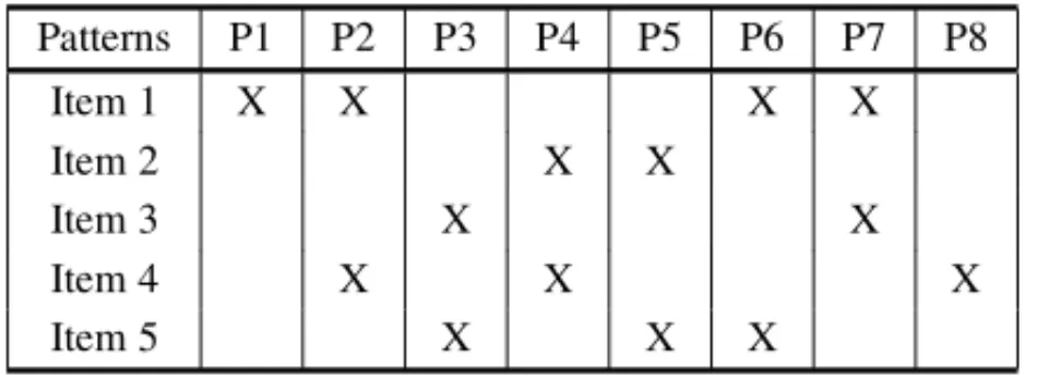
Table 1– An example of the MOSP with 8 patterns and 6 items.
Items Patterns
P1 P2 P3 P4 P5 P6 P7 P8
1 1 0 0 1 1 0 0 0
2 1 1 0 0 0 0 0 1
3 0 0 1 1 0 0 0 0
4 1 1 1 0 1 0 1 0
5 0 1 0 1 1 1 0 0
6 0 0 0 0 0 1 1 1
Items Patterns
P1 P2 P3 P4 P5 P6 P7 P8
1 1 0 0 1 1 0 0 0
2 1 1 0 0 0 0 0 1
3 0 0 1 1 0 0 0 0
4 1 1 1 0 1 0 1 0
5 0 1 0 1 1 1 0 0
6 0 0 0 0 0 1 1 1
#open
3 4 5 5 4 4 3 2
stacks
Items Patterns
P4 P5 P3 P1 P2 P6 P7 P8
1 1 1 0 1 0 0 0 0
2 0 0 0 1 1 0 0 1
3 1 0 1 0 0 0 0 0
4 0 1 1 0 1 0 1 0
5 1 1 0 0 1 1 0 0
6 0 0 0 0 0 1 1 1
#open
3 4 4 4 3 4 3 2
stacks
(a) (b)
Figure 1– Two solutions for the Pattern Sequencing Problem.
MOSP has been proved to be a NP-hard problem [28]. Besides the applications referred to above, it arises in production planning (for rapidly fulfilling the customers’ orders) [36], and also in other fields such as VLSI Circuit Design with the Gate Matrix Layout Problem and PLA Folding [28], and in classical problems from Graph Theory presented in Section 3.8 such as Pathwidth, Modified Cutwidth and Vertex Separation.
2.1 Other pattern sequencing problems related to MOSP
The Minimization of Discontinuities Problem (MDP) consists in finding a sequence to process the cutting patterns such that the number of discontinuities is minimum. We say that a disconti-nuityoccurs when an item that is being cut in a given pattern is not cut in the following pattern and is cut again later. The difference from the previous problem is that the duration of the discon-tinuities does not influence the cost of the solution, just its existence. This is a NP-hard problem, and it is also known in the literature as the Consecutive Blocks Minimization Problem [17]. Another problem is the Minimization of Tool Switches Problem (MTSP). This is a job scheduling problem that arises in flexible manufacturing machines, and has been applied, for instance, in the metal working industry and in the assembling operations of printed circuit boards. Machines in such systems are capable of different tasks, but may need a certain combination of tools. This problem considers machines that can hold a set of tools, which can be changed in order to have the adequate set of tools for each job. As these machines only have a capacity forC tools simultaneously, some tool switching must be made between different tasks sometimes. These tool changing operations may include retrieval from storage, transportation, loading and calibration, and have a cost proportional to the number of switches. The MTSP problem consists of finding a sequence of the tasks, in order to minimize the number of tool switches. A link between MTSP and MOSP can be established considering the jobs as cutting patterns and the tools as items to be cut.
The MORP, the MDP and the MTSP are NP-hard problems that are not equivalent to the MOSP, and not even to each other. Linhares & Yanasse [28] presented counterexamples to all the equiv-alence conjectures, except for the equivequiv-alence between the MTSP and MDP. They proved that if MTSP is fixed parameter tractable (FPT), then MDP is also FPT. Yanasse [37] showed that, although the MOSP is not equivalent to the MTSP in a general case, they are equivalent when the optimum of the MOSP (denoted byC∗) equals the capacityCof the machine in the MTSP. IfC >C∗, an optimal solution for the MOSP is always optimal for the MTSP, but the converse is not true. IfC<C∗, an optimal solution for the MOSP may not be an optimal solution for the MTSP and vice-versa.
3 GRAPHS AND LAYOUT PROBLEMS
3.1 Basic Definitions
Agraph G =(V,E)consists of a setV (that we call the set ofverticesornodes) and a setEof tuples fromV ×V, i.e,E = {e= [vw] :v, w ∈V}(that we calledgesorarcs). An edge with both endpoints on the same vertex is called aloop. An edgee = [uv]is amultiedgeork-fold edgeif there are exactlykedgese1,e2, . . . ,ek such thate1=e2 = · · · =ek = [uv]. Fork=2,
ork=3, it is called a double edge, or a triple edge, respectively. We call a graph with no loops or multiedges asimple graph. In this work, all graphs are assumed to be simple graphs.
the number of edges wherev is a head is called theindegreeand denoted byindeg(v), and the number of edges wherevis a tail is called theoutdegreeand denoted byout deg(v). The graph G−1=(V,E−1)is said to be thereversalofGifE−1= {[uv] ∈V×V : [vu] ∈ E}.
A graphG =(V,E)is calledundirectedif E = E−1. A graphG=(V,E)is calledoriented
if E
E−1=∅. In this work, we will mostly use undirected graphs; for this reason, from this point forward, unless stated otherwise, by graph we mean an undirected graph, and we will use without distinction[uv]and[vu]. Two verticesv, w ∈ V areadjacentif[vw]is an edge. Two edges areadjacentif they share a common vertex.
The neighborhood of a vertex is the set of its adjacent vertices. In simple graphs, as edges from a vertex to itself are not allowed, one vertex does not belong to its own neighborhood. So it is also usual to define the closed neighborhood of a vertex if we want to include it. For a given vertex u ∈V, we define theneighborhoodoradjacency setofuas: N(u)= {v ∈ V : [uv] ∈ E}and define theclosed neighborhoodofvas: N[u] = {u}
N(u).
We define thedegreeof a vertex v ∈ V to be the number of times thatvis an endpoint of an edge. A graph is saidk-regularif every vertex has degreek. In a simple graph, the degree of a vertexvis also the cardinality ofN(v).
ThecomplementofGis the graphG=(V,E)whereE = {[uv] ∈V×V :u=v∧ [uv]∈/ E}. Hence the complement graph is formed by the vertices together with the missing edges. A graph iscompleteif every pair of distinct vertices is connected by one edge. The complete graph onn vertices is usually denoted byKn. In a simple graph, the number of all possible edges isn2
.
3.2 Graph Optimization Problems
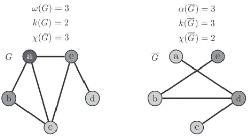
There are several problems in Graph Theory that are somehow related to the MOSP problem. The solutions to those problems provide graph measures that are illustrated in Figure 2.
Maximum Clique Number: find the set of vertices that form the largest clique in a graph. A cliqueis a set C of vertices of a graphG such that all pairs of vertices inC are adjacent. A cliqueC ismaximalif there is no clique ofGwhich properly containsC as a subset. A clique ismaximumif there is no clique ofGof larger cardinality. The size of the maximum clique in a graphGis called theclique number, and is denoted byω(G).
Minimum Clique Cover: find a set of cliques to cover all the vertices in the graph. Aclique coverof a graphGis a set of cliques such that every vertex inGbelongs to one clique. The size of the minimum clique cover is called theclique cover number, and is denoted byk(G). Maximum Independent Set:find the largest set of vertices nonadjacent to each other. Astable setorindependent setof a graphGis a subsetI of vertices such that no edge has both endpoints inI. The number of vertices in a stable set of maximum cardinality is called thestability number, and is denoted byα(G).
a
b
c
d
e
G
ω(G) = 3
k(G) = 2
χ(G) = 3
a
b
c
d
e
G
α(G) = 3
k(G) = 3
χ(G) = 2
Figure 2– Chromatic number, stability number, clique cover number and clique number of a graph and its complement graph.
partition of the verticesV =X1∪X2∪ · · · ∪Xk such that each Xi is a stable set. In a proper
k-coloring there is an assignment of integers{1,2, . . . ,k}(corresponding tokdifferent colors) to the verticesV such that for any edge the two endpoints have been assigned different colors. The smallest numberk such asGhas ak-coloring is called thechromatic numberofGand is denoted byχ(G).
Given a graphG=(V,E)and a subsetSofV,S is a clique ofGif and only ifS is a stable set ofG. As a consequence of this, for any graphG, we have:
ω(G)=α(G)
Since every vertex of a maximum stable set must be contained in a different partition segment in any minimum clique cover, it is valid that:
α(G)≤k(G)
As a stable set in a graphGcorresponds to a clique in the complement graphG, we have, for any graphG, the equality:
χ(G)=k(G)
For any graphG, there is also a lower bound for the chromatic number
ω(G)≤χ(G),
because if it contains a clique of sizekthen we need at leastkdifferent colors to color the vertices in that clique.
3.3 Chordal Graphs
Apathis a sequence of vertices[v0, v1, . . . , vk]such that[vi−1vi]is an edge fori =1, . . . ,k
and itslengthis the number of edges in the sequence. If no vertex is repeated, it is called asimple path. A graph isconnectedif there exists a path from any vertex to any other vertex in the graph. Aconnected componentof a graph is a maximal subgraph that is connected. A path that begins and ends at the same vertex is called acycle. If no vertex occurs more than once, the cycle is called asimple cycle. A graph without any cycle is called aforest. A graph withn vertices is a treeif it is a forest and it has exactlyn−1 edges.
A simple cycle[v0, v1, . . . , vk, v0]is said to bechordlessif[vivj]∈/ Efori and j differing by
more than 1 modk+1. The chordless cycle onnvertices is usually called an-cycleand denoted byCn.
Definition 1.A graph is achordal graphif it does not contain an induced k-cycle for k ≥4. The name “chordal” comes from the fact that in every simplek-cycle withk≥4 that may exist in this graph, there must be achord, which is an edge between two non-consecutive vertices of the cycle. Because of its geometric properties, these graphs are also calledtriangulatedgraphs. Being chordal is a hereditary property inherited by all the induced subgraphs ofG.
3.4 Perfect Elimination Order
Chordal graphs can be recognized by finding a special type of vertices and applying an iterative procedure to its induced subgraphs.
Definition 2. A vertexv ∈ V is calledsimplicialif its neighborhood N(v)induces a complete subgraph of G, i.e. N(v)is a clique (not necessarily maximal).
From Dirac (1961), as cited in [18], it is known that simplicial vertices appear in all chordal graphs:
Theorem 1. Every chordal graph G has a simplicial vertex and if G is not a complete graph then it has two nonadjacent simplicial vertices.
Definition 3.Given a graph G =(V,E), such that|V| =N , alinear orderingof the vertices is a bijective functionϕ : V → {1, . . . ,N}. Thereversed linear ordering,ϕR :V → {1, . . . ,N}, is a linear ordering such thatϕR(u)=N−ϕ(u)+1.
A linear ordering of the vertices of a graph is sometimes called alayoutof the graph, a number-ing, alinear arrangement or alabelingof the vertices. We will also use the symbol≺to express the linear ordering on the set of vertices.
Definition 4. Given a graph G = (V,E)and a linear orderingϕ of its vertices, we say that vertex iprecedesvertex j , and denote by i≺ j , ifϕ(i) < ϕ(j). We denote the set of predecessors of a vertex by Pred(i)= {j ∈N(i):ϕ(j) < ϕ(i)}and the set of successors by Succ(i)= {j ∈
This ordering of the vertices can also lead to edge directions, directing the edge[i j]ifi ≺ j. If the graph is simple then|Pred(v)| =indeg(v)and|Succ(v)| =out deg(v), where|.|designates the cardinality of the set.
Definition 5. A linear orderingσ = [v1, v2, . . . , vn]of the vertices of a graph G =(V,E)is
called aperfect elimination scheme(or p.e.s.) if eachvi is a simplicial vertex of the induced
subgraph Gvi,...,vn.
A simplicial vertex can start a perfect elimination scheme, or start a similar linear ordering called a perfect elimination order:
Definition 6.[4] Aperfect vertex elimination order(orp.e.o.) is a linear ordering of the vertices of the graph in which the sets of predecessors of each vertex Pred(i)form a clique,∀i∈V .
In a perfect elimination scheme, each of the setsSucc(i)are complete sets. In a perfect elimina-tion order, the setsPred(i)are complete. This means that ifϕis a perfect elimination order, then the reversed orderingϕRmay not be a perfect elimination order as well, but it will be a perfect elimination scheme. The reason for this is because the set of predecessors of a vertex for a given linear ordering is the set of successors of that vertex for the reversed linear ordering, since:
ϕR(j) > ϕR(i)⇔N−ϕ(j)+1>N−ϕ(i)+1⇔ϕ(j) < ϕ(i)
Definition 7. A subset S ⊂ V is avertex separator for nonadjacent vertices a and b (or an
(a,b)-separator) if the removal of S from the graph separates a and b into distinct connected components. If no proper subset of S is an(a,b)-separator, then S is aminimal vertex separator for a and b.
All the minimal vertex separators of a chordal graph are cliques [18]:
Theorem 2.Let G be an undirected graph. The following statements are equivalent:
(i) G is chordal;
(ii) G has a perfect vertex elimination scheme. Moreover, any simplicial vertex can start a perfect scheme;
(iii) Every minimal vertex separator induces a complete subgraph of G.
3.5 Comparability Graphs
Comparability graphs are a special case of graphs that can be transitively oriented.
Definition 8.Acomparability graphis an undirected graph G =(V,E)in which each edge can be assigned a one-way direction in such a way that the resulting oriented graph(V,F)satisfies:
[uv] ∈ F∧ [vw] ∈F ⇒ [uw] ∈ F ∀u, v, w∈V
This transitive orientation is acyclic, i.e., a comparability graph does not contain any directed cycle. With the orientation fixed, a comparability graph is also called apartially ordered setor poset.
A graphGis said aco-comparability graphifGis a comparability graph.
3.6 Interval Graphs
Definition 9. Aninterval graphis an undirected graph G such as its vertices can be put into a one-to-one correspondence with a set of intervals I of a linearly ordered set (like the real line) such that two vertices are connected by an edge of G if and only if their corresponding intervals have nonempty intersection. I is called aninterval representationfor G.
Graphs which represent intersecting intervals on a line are an useful concept for us because if we associate each open stack of our MOSP problem to an interval in the real line (the interval of time that the stack stays open), then we can associate a solution of the MOSP to an interval representation of an interval graph.
Being an interval graph is a hereditary property, i.e., an induced subgraph of an interval graph is an interval graph. Recognizing whether a given graph is an interval graph can be carried out in linear time.
Besides the definition, there are theorems that characterize interval graphs. Lekkerkerker & Boland (1962) characterization [27] focuses on the fact that an interval graph cannot branch into more than two directions nor circle back onto itself.
Theorem 3. [18] An undirected graph G is an interval graph if and only if the following two conditions are satisfied:
(i) G is a chordal graph and;
(ii) any three vertices of G can be ordered in such a way that every path from the first vertex to the third vertex passes through a neighbor of the second vertex.
AT-freeif it contains no asteroidal triple. Using this terminology, Theorem 3 states that a graph is an interval graph if and only if it is chordal and AT-free. The AT-free structure of interval graphs has been used to develop a linear time algorithm to recognize interval graphs [9].
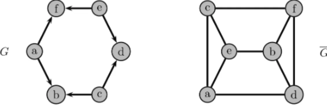
The graph in Figure 3 is not an interval graph because it contains an asteroidal triple: the vertices a,b,c. A path fromatobisa,d,g,e,bwhich avoidsN(c)= f.
Figure 3– Not an interval graph.
Some other characterizations of interval graphs are known, namely the following theorem (Gil-more & Hoffman, 1964) as cited in [18]:
Theorem 4.Let G be an undirected graph. The following are equivalent:
• G is an interval graph;
• G is chordal and G is a comparability graph;
• The maximal cliques of G can be linearly ordered such that, for every vertexv of G, the maximal cliques containingvoccur consecutively.
Note that, in this theorem, it is stated that the complement of an interval graph is a comparability graph. However, the reverse does not hold, i.e., the complement of a comparability graph is not always an interval graph. An example is shown in Figure 4.
Figure 4–Gis a comparability graph butGis not an interval graph.
Definition 10.A matrix of zeros and ones is said to have theconsecutive 1’s property for columns if its rows can be permuted in such a way that the 1’s in each column occur consecutively.
Theorem 5. [16] An undirected graph G is an interval graph if and only if its clique matrix M has the consecutive 1’s property for columns.
This property is not only present in the clique matrix, but also in the adjacency matrix of an interval graph (Tarjan, 1976) as cited in [5].
Theorem 6. G =(V,E)is an interval graph if and only if there exists a linear ordering of G such that the associated adjacency matrix A verifies:
∀i∈ {1, . . . ,N} ai j =1for j= fi(A), fi(A)+1, . . . ,i
where fi(A)=min{j :ai j =0}
There is an alternative characterization of interval graphs, due to Olariu [9], that uses the linear ordering of the vertices, and is illustrated in Figure 5:
Figure 5– Olariu’s characterization of interval graphs.
Theorem 7.A graph G =(V,E)is an interval graph if and only if there exists a linear ordering
ϕ : V → {1, . . . ,N}such that∀i,j,k∈ V :ϕ(i) < ϕ(j) < ϕ(k)we have[ik] ∈E ⇒ [i j] ∈
E.
We will use this characterization to develop an integer programming model for the MOSP. Start-ing from a graph that represents the MOSP instance, new edges are added to the MOSP graph to assure that the graph of the solution is an interval graph, as described in detail in Section 4. Issues related to adding edges (edge completion) are addressed in Section 3.10.
The ordering of the maximal cliques in an interval graph referred to in Theorem 4 will allow us to set an interesting ordering for the vertices, using the following theorem from Biedl [4]. Theorem 8.An interval graph G has an interval representation such that all endpoints of inter-vals are distinct integers.
By using, for instance, the left endpoints of the intervals, we can define a natural ordering of the vertices of the graph: declarei ≺ j if the left endpoint of intervali precedes the left endpoint of interval j. Therefore, we can assign edge directions based on this vertex order, choosing to direct each edge from left to right, directing the edge[i j]ifi ≺ j.
Theorem 4 occurs consecutively and has the form Pred(u)∪ {u}for some vertexu. But not every set Pred(u)∪ {u}has to be a maximal clique: Letv1, . . . , vn be a perfect elimination
order. ThenC =Pred(vi)∪vi is not a maximal clique if and only if there exists a successorvj
ofvi such thatviis the last predecessor ofvj andindeg(vj)=indeg(vi)+1.
The perfect elimination order of the vertices of the graph can give origin to a linear ordering of the left endpoints of the intervals of an interval representation constructed for the graph. Note that if a graphGhas a perfect elimination order, thenGis chordal.
Given an interval graph and some vertexvirepresented by an interval that starts atsi,Pred(vi)is
the set of all vertices representing intervals that start beforesiand do not end beforesi. Therefore,
all these intervals contain the pointsi, and hence overlap each other, which means thatPred(vi)
is a clique and therefore the vertex order is a perfect elimination order [4].
Figure 6– The p.e.o.a,b,c,d,e, f gives the linear ordering of the left endpoints of the intervals.
The vertex ordering defined by the left endpoints of the intervals creates in fact the sequence of cliques that will appear in the interval graph, and that we are interested in finding, in order to discover the solution of a MOSP problem.
It is known that an interval graphHis chordal and it has at least two simplicial vertices where a perfect vertex elimination scheme can be started. Locating a simplicial vertex and eliminating it will create another simplicial vertex and its subsequent elimination and so on.
A perfect elimination scheme is not appropriate for ordering the left endpoints of the intervals, as can be confirmed in Figure 7. In fact, the order in which the intervals must start can be set by following the reverse order of the eliminated vertices, which is a perfect elimination order.
Figure 7– The p.e.s. f,e,d,c,b,ais not adequate for ordering the left endpoints of the intervals.
Although every interval graph has a perfect elimination order, the reverse does not hold. For example, trees may not be interval graphs (for example Figure 3), but have a p.e.o. because they are chordal graphs.
3.7 Perfect Graphs
Interval graphs are part of a more general class of graphs beautifully called perfect graphs. Definition 11.A graph G=(V,E)is aperfect graphif it satisfies both the properties:
(i) ω(GA)=χ(GA) ∀A⊆V ;
(ii) α(GA)=k(GA) ∀A⊆V .
Actually, it is sufficient to show one of these properties, as the Perfect Graph Theorem (Lov´asz, 1972) implies that these two properties are equivalent.
Theorem 9. (Perfect Graph Theorem)[18] A graph G is perfect if and only if its complement G is perfect.
An odd length cycle is called anodd holeand its complement is called anodd anti-hole. Conjecture 1. (Strong Perfect Graph Conjecture)A graph is perfect if and only if it does not have an odd hole or an odd anti-hole as an induced subgraph.
This conjecture was posed in 1961 by Claude Berge and proved by Chudnovsky, Seymour, Robertson and Thomas in 2003 [8].
Theorem 10.[18] Every comparability graph G is a perfect graph.
To see this let us define on the oriented graphG=(V,F)the height function h(v)=
0 ifvis a sink 1+max{h(w): [vw] ∈ F} otherwise
A sink is a vertex of the oriented graph that has outdegree zero. This is always a proper coloring of the vertices of a graph. The number of colors used is equal to the number of vertices in the longest path ofF.
If Gis a comparability graph with a transitive orientation F, every path in F will correspond to a clique ofGbecause of transitivity. So in this case, the height function will yield a coloring which uses exactlyω(G)colors, which is the best possible. As being a comparability graph is hereditary, the clique number and the chromatic number are also equal for all induced subgraphs of G. As the complement of an interval graph is a comparability graph, then interval graphs are perfect.
3.8 Graph Layout Measures
The linear ordering of the vertices of a graph is also called the layout of the graph, because when the vertices are arranged by that ordering, there are several measures that naturally can be taken and used to describe geometric properties of the graph.
Treewidth
The treewidth is a layout measure that counts the number of adjacent vertices of a given graph Gthat we can group together and replace each group by a vertex of a treeT appropriately built fromGby connecting the vertices of the treeT that are covering the same vertices of the graph G.
Definition 12. Atree decompositionof a graph G =(V,E)is a tree T = (I,F)where each node i∈ I has a label Xi ⊆V such that:
•
i∈I Xi=V . We say thatall vertices are covered.
• For any edge[vw]there exists an i ∈ I withv, w∈ Xi. We say thatall edges are covered. • For anyv ∈ V the nodes in I containingvin their label form a connected subtree of T .
We call this theconnectivity condition.
Figure 8– A graph with a tree decomposition of width 2 [6].
A given tree can be the tree decomposition of several different graphs. The graph implied by a tree decomposition is the graph obtained by adding all edges between vertices that appear in a common label.
Definition 13. Given a tree decomposition T =(I,F), thewidth of the tree decompositionis maxi∈I|Xi| −1.
Definition 14.Thetreewidthof a graph G is the minimum k such that G has a tree decomposition of width k:
T W(G)=min
max
i∈I |Xi| −1:T =(I,F)is a tree decomposition of G
Thetreewidth problemconsists in, givenk≥0 and a graphG, finding ifT W(G)≤k.
Notice that each clique in a graph must be part of at least one node in the tree decomposition, and hence the clique number minus one is a lower bound for treewidth. For this reason, all trees have treewidth 1.
Lemma 1.[6] If G is chordal then G has a tree decomposition of widthω(G)−1.
The minimum degreeδ(G)of the vertices of a graphGand thedegeneracyof a graphδD(G), defined byδD(G):=max
H⊆Gδ(H), are lower bounds for the treewidth: δ(G)≤T W(G)
δD(G)≤T W(G)
Computing the treewidth is a NP-hard problem [1, 7].
Pathwidth
A particular case occurs when we require the decomposition to be a path, which is called apath decomposition of width k.
Definition 15.A graph G haspathwidthPW(G)bounded by k if G has a tree decomposition T of width k such that T is a path.
Computing the pathwidth is NP-hard in general but, for a given constantk, testing whetherGhas pathwidth bounded bykcan be done in linear time. From the definition, we immediately have T W(G)≤PW(G).
In [28], Yanasse and Linhares pointed out that the MOSP, the Gate Matrix Layout Problem (GMLP) and the Pathwidth are equivalent problems that have been studied independently in the literature. In fact, Kinnersley proved in [24] the equivalence between the Pathwidth and the Vertex Separation problem and showed that the GMLP cost of a graph equals its pathwidth plus one. Hence the pathwidth is equivalent to the MOSP. In fact, the pathwidth problem consists of finding an interval supergraph with the smallest clique number [15].
3.9 Linear ordering
Many graph layout problems involve finding a linear ordering of the vertices to optimize a given objective function. One example is theLinear Ordering Problem(LOP). It consists in finding a linear ordering of the vertices such that the number of directed edges in the graph that are not in accordance with this ordering is minimized. It belongs to the class of NP-hard combinatorial optimization problems, and its integer programming formulation and its polytope were studied in [13, 19, 34]. The decision variables are defined as:
xi j =
We will not present the LOP, but just focus on the constraints that define the linear ordering of the vertices:
xi j+xj i =1 ∀i,j ∈V,i< j (1)
xi j+xj k+xki ≤2 ∀i,j,k∈V,i < j,i<k,j =k (2)
xi j ∈ {0,1} ∀i,j ∈V,i< j (3)
The first set of contraints (1) means that, in the linear ordering, either vertexiis before jor vice versa, reducing this to a minimal equation system. The inequalities (2) are called the 3-dicycle inequalities and along with the first equations guarantee that the graph is free from cycles. The last inequalities (3) are called hypercube constraints.
The inequalities (2) and (3) define facets of the linear ordering polytope [19]. Forn ≤ 5, the inequalities (1)-(3) are sufficient to describe the linear ordering polytope, but forn > 6 more facet defining constraints are needed [34].
3.10 Edge Completion Problems
Anedge completion problemconsists in, given a graphG=(V,E), finding asupergraph H = (V,E∪F)with the same set of vertices V and an extra set of edges F (called thefill edges) that are added to the previously existing onesE, chosen in a way such as H belongs to some predefined class of graphsC, like chordal graphs, interval graphs, split graphs, while optimizing
some cost function, like the number of added edges|F|, or the clique number of the graphω(H). Note that we considerE∩F =∅for distinguishing the fill edges in F from the original ones inE.
Several edge completion problems have been studied in literature, concerning different aimed classes of graphsC and different cost functions to optimize. The class of chordal graphs is the
most addressed. If the desired supergraphH ofGis required to be chordal,His called a trian-gulationofG. Another class for edge completion problems is the class of interval graphs. If the supergraph H is required to be an interval graph, the edge completion problem is called an in-terval graph completion. Edge completion problems whereCis the class of AT-free graphs [25],
split graphs [21], proper interval graphs [23] and comparability graphs [22] have also been studied.
Minimum vs. Minimal Edge Completion Problems
There are also variants depending on the selected cost function. For example, if the cost function is one less than the size of the largest cliqueω(H)−1, its optimization can lead to problems like treewidth or pathwidth. There exists a triangulationH =(V,E∪F)ofGwith maximum clique sizesk+1 if and only if the treewidth of G is k [6]. By Lemma 1, thetreewidth of a graphG coincides with minHω(H)−1 for all triangulationsH ofG. The treewidth is the
The pathwidth problem consists of finding an interval graph completion that minimizes also
ω(H)−1.
AminimumC-completion ofG=(V,E)is a supergraphH=(V,E∪F)∈C that minimizes
the number of added edges|F|. A triangulation ofGthat minimizes the number of added edges
|F|is called aminimum triangulationorminimum fill-in, and an interval graph completion that minimizes the number of added edges|F|is called aminimum interval graph completion(IGC). The minimum fill-in is a NP-hard problem, as well as the minimum interval completion, the treewidth and the pathwidth problems. Most researchers choose to address an easier problem that is related to these, which is to find aminimal fill-inor aminimal interval graph completion[20]. A minimalC-completion ofG=(V,E)is a supergraphH =(V,E∪F)∈C such that every
H′=(V,E∪F′)forF′⊂Fis not aC-completion ofG. In the case of minimal triangulations,
it is equivalent to saying that the removal of a single fill edge of a solutionHwill result in loosing chordality. For the problem of finding a minimal interval graph completion that does not hold, i.e. removing a single fill edge of a minimal interval graph completion H ofG might give a subgraph that it is not interval, but removing more than a single fill edge might give an interval graph completion ofG.
A solution to the minimum completion problem must always be a minimal completion, but min-imal triangulations or interval completions do not imply that the number of edges is minimum.
4 MOSP GRAPH
A MOSP problem with at most two different items per pattern can be represented through a graph that associates vertices to orders and arcs to patterns [38]. By making each item correspond to a vertex, and considering two vertices to be adjacent if and only if the corresponding items are simultaneously present in a pattern, we obtain aMOSP graph.
The condition of having at most two different panel types per pattern represents no loss of gen-erality, because a solution of the general case can be transformed in a solution of the first case in polynomial time (and vice-versa) [38]. Given a general MOSP problem, a MOSP graph can be obtained by introducing a clique of sizekfor each pattern composed bykpanel types. By analogy to each arc in the clique, this pattern can be divided in subpatterns with at most 2 items in each, transforming it in a MOSP graph corresponding to a problem where there are at most 2 items per pattern. In [38], Yanasse proves that the maximum number of stacks in both problems is the same.
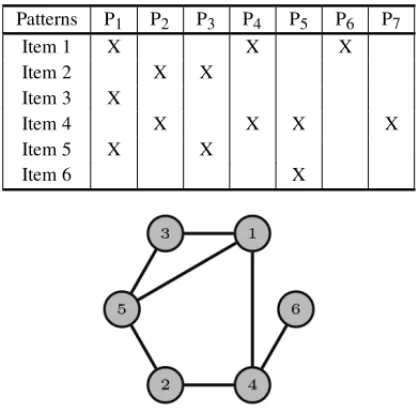
Table 2– An instance of the MOSP with 7 cutting patterns and 6 items.
Patterns P1 P2 P3 P4 P5 P6 P7
Item 1 X X X
Item 2 X X
Item 3 X
Item 4 X X X X
Item 5 X X
Item 6 X
Figure 9– MOSP Graph of the instance in Table 2.
Furthermore, Yanasse showed that it is possible to take a solution for the ordering of the vertices of the MOSP graph and construct a sequence for the corresponding cutting patterns [38]. A linear ordering of the vertices sets an ordering for the opening of the stacks; following this ordering, a pattern will be put in the sequence when it is the first time that all vertices corresponding to all items present in that pattern have been opened.
Some simplifications are possible. When there are some patterns with only one item that is also produced by another pattern, we say that the first pattern is contained in the second pattern. It has been proved by Yanasse [37] that this type of patterns can be removed from the problem and inserted later in the solution just before the patterns in which they were contained. It happens, for instance, with patterns P6 or P7 in Table 1. Each pattern should be sequenced just before the first of the patterns containing that item, and the number of simultaneously open stacks will not increase [37]. Therefore, this instance can be reduced to only five relevant patterns (P1, P2, P3, P4 and P5) generating the same graph.
There are other situations in which patterns can be removed from the original problem before solving it, and then inserted later in the solution. Items that are present in just one pattern will appear in the graph as isolated vertices if that pattern does not include any other item. In this case, that pattern can be the first or last in the sequence, and it will open and close a stack without any other stacks open at that same time, so it does not increase the maximum number of simultaneously open stacks.
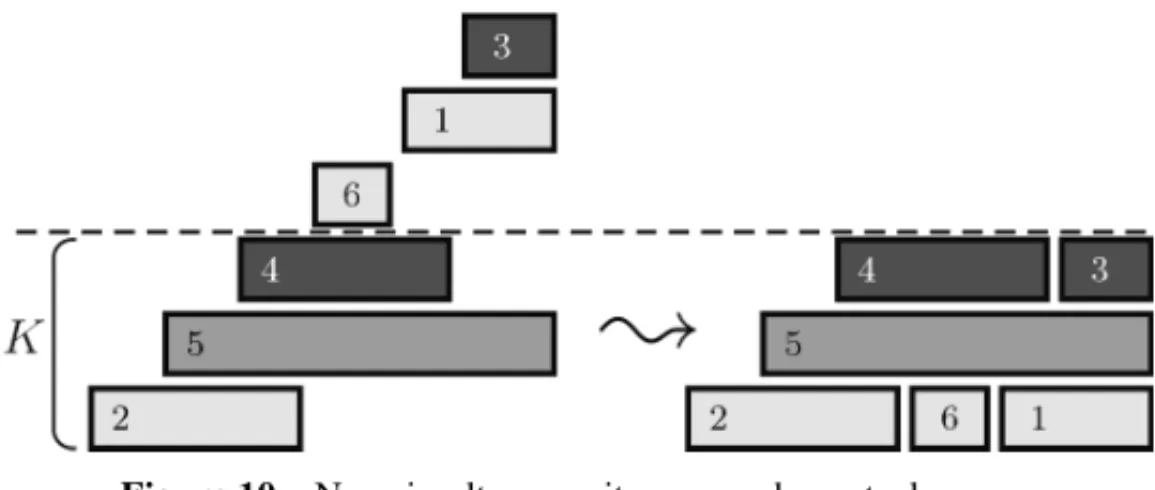
For the example in Table 1, if the patterns are sequenced by the ordering P1P2P3P4P5P6P7,
patternsP3P7P2P5P6P4P1. As there are some stacks that are not simultaneous at any time, like
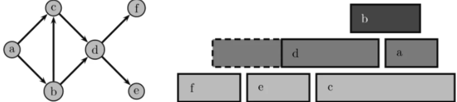
3 and 4, or 1, 2 and 6, those stacks can use the same stack space; hence this sequence of patterns gives a maximum of three simultaneously open stacks, which is the optimum for this instance, as can be observed in Figure 10.
Figure 10– Non simultaneous items can share stack space.
This means that it is natural to associate the lifetime of a stack in the solution with intervals of time measured not in minutes or hours but measured in terms of the patterns in the sequence. We saw that we can start solving a MOSP problem with a graph, and that in the solution of the problem we can consider an interval for the time that each stack is open. By associating each open stack of our MOSP problem to an interval in the real line (the interval of time that the stack stays open), we can associate a solution of the MOSP to an interval representation of an interval graph. An interval graph can be associated to the set of intervals in the solution and the MOSP graph will be modified in order to become an interval graph. We will use some properties of interval graphs to find the solution of MOSP instances.
For the example in Figure 9, the interval graph corresponding to the solution displayed in Fig-ure 10 has the same vertices and edges of the MOSP graph and two additional edges, as depicted in Figure 11. This is an interval graph completion (as explained in Section 3.10) of the original MOSP graph. The fill edge [54]was added to make the graph chordal, because it is a chord of the previous 4-cycle 1,4,2,5. The fill edge[56]was added to eliminate the asteroidal triple 3,2,6, transforming the MOSP graph in an AT-free graph. In the original MOSP graph 3,2,6 is an AT because 3,5,2 is a path from vertex 3 to vertex 2 that does not pass through any neighbor of vertex 6. With the edge[56]now vertex 5 is a neighbor of vertex 6.
As discussed in Section 3.6, the vertex order defined by the left endpoints of the intervals is related to the sequence of cliques that will appear in the interval graph of the solution of a MOSP problem.
5 AN INTEGER PROGRAMMING MODEL FOR THE MOSP
Given an instance of the problem, we first build a MOSP graphG =(V,E), associating each item cut from the patterns to a vertex and creating an arc joining vertexiandjif and only if items i and j are cut from the same pattern. This graph may not be an interval graph at the start, but we will add some arcs to it in such a way that it will become one. We need this graph to become an interval graph because, if we associate each item to the interval of time in which the stack of that item is open, we can use the graph to model what intervals should occur simultaneously and what intervals should precede others. Each arc of the future interval graph means that, for a period of time, the two stacks (the 2 vertices that are endpoints of the arc) will remain both open. The initial graph contains only the arcs that must be there, in any possible sequence in which the patterns can be processed. The remaining arcs that are added later to the graph will differ according to the sequence of the patterns. It is the choice of these arcs that defines which are the other simultaneously open stacks.
Our model consists in finding out which edges should be added to the original MOSP graphG= (V,E)in order to get an interval graphH =(V,E∪F)that minimizes the maximum number of simultaneously open stacks. We will use the characterization in Theorem 7 to guarantee that the graph obtained in the solution of the problem is an interval graph.
5.1 Decision Variables
We set an ordering for opening the stacks by assigning a number to each item cut, with a bijective functionϕ:V → {1, . . . ,N}. This linear ordering of the vertices is set by the decision variables xi j:
xi j =
1 ifϕ(i) < ϕ(j)
0 otherwise ∀i,j ∈V
Notice thatxii =0 for anyi ∈ V and also that we havexi j =1 ⇔ xj i =0. These variables
set an orientation into the arcs, to keep track of the sequence of the items. Ifxi j =1 then itemi
starts being cut before the item j, even though the corresponding stacks may overlap or not, i.e., in spite of having an arc between the two vertices or not.
Other decision variables will be used to identify the arcs that are added to the original graph G=(V,E)to get an interval graphH =(V,E∪F)and, together with variablesx, determine which intervals will overlap. To decide which of these additional arcs are to be added, we define a variableyi j for each arci j that did not exist before in the graph:
yi j =
1 if[i j]∈/ Fandϕ(i) < ϕ(j)
Note thatyi j is 1 when the arc[i j]is NOT added. Variablesydepend on the linear ordering of
vertices, so it follows that there is an anti-reflexive relationyi j =1⇒ yj i =0. Whenyi j =1,
the arc[i j]is not needed in the interval graph, so, by definition of interval graph, if there is not an arc[i j], then the intervalsi and j do not intersect. Consequently, one of the intervals should finish before the other one starts. Asi≺ j, the intervaliopens and finishes before the interval j starts. It means that the stacks for itemsi and jwill never be open at the same time, so they can share the same stack space, as seen in Figure 12.
Figure 12– Intervaliopens and closes before jstarts.
As one of the conditions for the variable yi j to be equal to 1 is that vertexi precedes vertex j,
equivalent to saying thatxi j =1, then we must have:
yi j ≤xi j ∀i,j∈ V :i = j,[i j]∈/ E (4)
Whenyi j =1, the arc[i j]is not needed in the interval graph; so, by definition of interval graph,
if there is not an arc[i j]then intervalsiand jdo not intersect. Consequently, one of the intervals should finish before the other one starts. Asyi j ≤ xi j, we must also havexi j =1, determining
that the intervali opens and finishes before the interval jstarts.
5.2 Edge Completion to Obtain an Interval Graph
To guarantee that the graph H = (V,E ∪F)is an interval graph, we use in the model the characterization given in Theorem 7, to express relations between the binary variablesyi jandxi j.
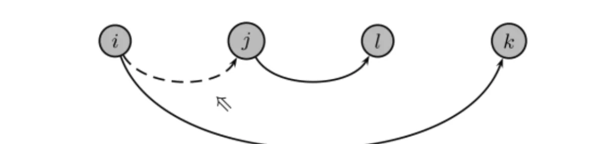
Recall that Olariu’s Theorem characterizes interval graphs as graphs in which the vertices can be linearly ordered in such a way that, for any three verticesi, j,ksuch thati ≺ j ≺k, if[ik] ∈E then[i j] ∈ E, as shown in Figure 5.
We will consider three different vertices i,j,k ∈ V that do not form a clique in the original MOSP graph, and analyze in what circumstances the arcs[i j]have to be added. Let us separate the analysis in two cases: (i) arc[ik] ∈E and (ii) arc[ik]∈/ E.
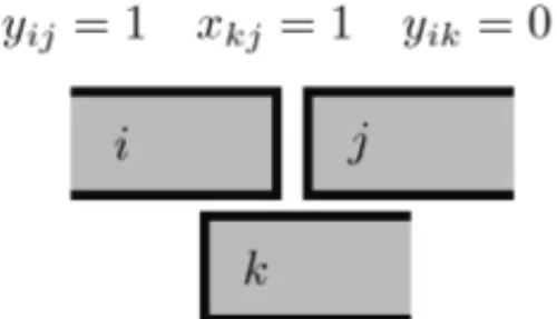
Case 1: arc[i k] ∈E
Let us suppose that arc[i j]∈/ E, otherwiseH already obeys the condition needed in an interval graph. Ifi ≺ j ≺ kthen as[ik] ∈ E then for H to be an interval graph it must be[i j] ∈ F. When xi j = 1, an arc[i j]will belong to the graph H if yi j = 0. Clearly, if xi j = 1, then
yj i = 0. Olariu’s characterization can be expressed as follows. For each arc [i j] ∈/ E, the
value of the corresponding variableyi j should obey: yi j+xi j +xj k ≤2. The inequality states
that, if vertexi precedes j and vertex j precedes k, or equivalentlyxi j = xj k = 1, then the
This inequality can be strengthened as follows. Combine the inequality with the inequalities yi j ≤xi j andxj k ≤1 to obtain:
yi j +xi j+xj k ≤ 2
yi j−xi j ≤ 0
xj k ≤ 1
2yi j+2xj k ≤ 3
Divide both sides by 2 and, as the variables are integers, we can round the fractional part of the right hand side to obtain a stronger inequalityyi j +xj k ≤1. Because xk j =1−xj k, this
inequality is equivalent to the constraint in binary variables equivalent to the logical implica-tionyi j ⇒xk j:
yi j ≤xk j ∀i,j,k∈V,[i j]∈/ E,[ik] ∈E (5)
We have assumed thati ≺ j ≺ kbut this is valid too ifi ≺ j butk ≺ j, because we have xk j =1. If j ≺ i thenxi j =0 and by (4) we haveyi j =0 and the inequality is also valid. In
fact, when there is the arc[ik]in the initial graph, but not the arc[i j](it is indifferent if the arc
[k j]exists or not), this means that intervalsiandkmust overlap.
Ifyi j =1, then intervaliwill close before interval jstarts. As intervalkmust overlap intervali,
because[ik] ∈ E,kmust be already open when j starts. So we must havexk j =1, as depicted
in the next figure.
In the example presented in Section 4, the vertices 2, 6 and 4 form a set in these conditions, because[24] ∈ E but[2,6] ∈/ E. Hence, in the model for this example there is the inequality y26 ≤ x46. In the solution, as can be observed in Figure 10, interval 2 opens and closes before
interval 6 opens (y26 =1) and the linear ordering is 2≺4≺6.
Note that if both arcs[ik]and[j k] ∈E andxik =xj k =1, then bothiand jare predecessors
ofk. Following the definition of an interval graph, the predecessors ofk must form a clique. In the model, that is equivalent to havingyi j = yj i =0, meaning that there should be an arc
xj k =1 means that interval jopens before intervalk. As[ik] ∈ E, intervalkmust overlap with
intervali, even ifiopens beforejstarts. Then intervalicannot be closed beforejstarts because i has to wait tillkstarts. The situation is captured in the following picture.
In the example being analyzed, the set of vertices 5, 4 and 1 will admit in the model the inequality y54 ≤ x14. As in the solution the linear ordering of these vertices is 5≺4 ≺1, this inequality
forces y54=0 meaning that the arc[54]is added to the graph, as can be seen in Figure 11.
Case 2: arc[i k]∈/ E
On the other hand, the arc[ik]may not be originally in the set of arcsE, but it may be added, as a result of other constraints in the model. In this situation,[ik] ∈ F, we will have the variableyik
taking the value 0, and the function(xik−yik)taking the value 1, meaning that arc[ik]is added to
the set. In this second case, also consider[i j]∈/ E, because otherwise the result was guaranteed. Clearly, Olariu’s characterization should also apply to this case. Therefore, for each arc[i j]∈/ E, the value of the corresponding variableyi jcan be constrained asyi j+(xik−yik)+xj k ≤2. The
inequality states that, if both verticesiand j precedek, or equivalentlyxik=xj k=1, when the
variableyikis set to 0 by another constraint (meaning that the arc[ik]is added to the graphG)
then the variableyi jmust also be equal to 0 (meaning that[i j] ∈ Fori does not precede j).
This inequality can be strengthened as follows. Combine the inequality with the following in-equalities from the linear ordering polytope, as well as a non-negativity constraint, to obtain:
yi j+xik−yik +xj k ≤ 2
xi j−xik +xj k ≤ 1
yi j−xi j ≤ 0
−yik ≤ 0
2yi j+2xj k−2yik ≤ 3
By dividing both sides by 2, and rounding the fractional part of the righthand side, we obtain yi j+xj k−yik ≤1. This inequality is equivalent to a constraint in binary variables equivalent
to the logical implicationyi j ⇒xk j ∨yik:
yi j≤xk j +yik ∀i,j,k∈V,[i j],[ik]∈/ E (6)
Supposing thati ≺ j ≺k, this means thatxj k =1 or equivalentlyxk j =0. If we decide to add
the arc[ik], thenyik =0 and the inequality forces yi j =0, meaning that we must also add the
This inequality is also true if the arc[ik] is not added because thenyik = 1 andyi j would be
free. This inequality is also valid in all other possible orderings of the verticesi,j,kas can be seen in Table 3.
Table 3– Possible cases when arc[i k] ∈F.
Vertices yi j ≤ xk j + yik
i≺ j≺k 0 0 0
i≺k≺ j free 1 0
j≺i≺k 0 0 0
j≺k≺i 0 0 0
k≺i≺ j free 1 0
k≺ j≺i 0 1 0
In the second, fifth and sixth cases (k ≺ j), adding the arc[ik] to the graph does not force to add the arc[i j]. In the remaining three cases where j ≺ i, the inequalityyi j ≤ xi j (4) forces
yi j =0.
In fact, ifyi j =1, meaning thati ends before j starts, thenxk j =1 meaning thatkshould start
before j, as shown in Figures 13 and 14, or yik =1, meaning thati should end beforekstarts,
as depicted in Figures 14 and 15.
Figure 13– Intervali closes before interval j opens, with in-tervalkbeing simultaneous to intervaliand opening beforej.
Figure 14– Intervalicloses before intervalsjandkopen, with intervalkopening before interval j.
In the example, the three vertices 6, 1 and 3 originate the inequalityy61≤x31+y63.
As in the solution the linear ordering of these vertices is 6≺ 1 ≺3, if the arc[63]was added, then the arc[61]should also be added. In this case, both arcs were not added, making these three variables equal to one.
5.3 Objective function
The position of vertex j in the linear ordering is found counting the number of vertices that precede it. For every vertex j, the sumN
i=1xi j counts how many vertices precede j, i.e., the
number of intervals that start beforei starts. On the other hand, variableyi j = 1 means that
vertexi closes before vertex j opens. For every vertex j, the sumN
i=1yi j counts how many
intervals finish before interval jstarts.
So, when vertex j opens, the number of intervals that are open at that instant is N
i=1xi j −
N
i=1yi j+1, where the constant 1 accounts for the vertex jitself. This leads to a set of functions
that can be used to evaluate the MOSP number:
N
i=1 i=j
xi j − N
i=1
[i j]∈/E
yi j +1≤K ∀j =1, . . . ,N (7)
Each function provides a lower bound for the MOSP, beingK the maximum of those functions. The objective function of the model is to minimize K. If one puts each interval in a line, as in Figure 16, the number of lines open when an interval starts is a lower bound for the maximum number of open stacks.
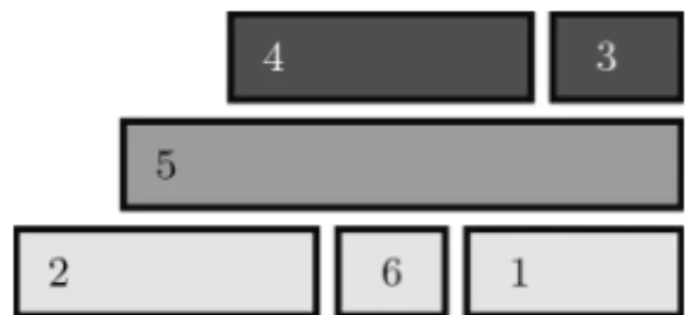
Figure 16– Optimal solution of the example from Table 2.
In the example presented before, when interval 5 starts, the number of open stacks turns to two, i.e., for j =5:
xi j −
which is a lower bound for the MOSP (which is three). The same inequality, corresponding to the moment that interval 1 starts, gives a better lower bound. At that instant, there are four intervals already open (2, 5, 4 and 6) but two of those have already closed (intervals 2 and 6). Hence the inequality is, forj =1:
xi j−
yi j+1=4−2+1=3≤3.
There are 6 cliques in the sequence of the perfect elimination order, such that every appearance of a vertex in these cliques is consecutive. The sequence of cliques is:
{2},{2,5},{2,5,4},{6,5,4},{1,5,4},{1,5,3}
The first 2 cliques are not maximal, but all the others are maximal with size 3, which is the optimum for this instance of the MOSP.
The value of the optimum of the MOSP is equal to the size of the largest clique in the solution graph,ω(H), and, because interval graphs are perfect graphs, it is equal to the chromatic number of the graph,χ(H), which is the number of colors needed to assign to the vertices of the graph such that there are no two adjacent vertices of the same color.
Our basic new mathematical formulation for the MOSP problem is: Minimize K
Subject to:
xi j +xj i =1 ∀i,j =1, . . . ,N withi = j (8)
xi j +xj k+xki ≤2 ∀i,j,k=1, . . . ,N withi = j =k (9)
yi j ≤xi j ∀i,j =1, . . . ,N withi = j and[i j]∈/ E (10)
yi j ≤xk j ∀i,j,k=1, . . . ,N with[i j]∈/ E,[ik] ∈ E (11)
yi j −yik ≤xk j ∀i,j,k=1, . . . ,N with[i j],[ik]∈/ E (12) N
i=1 i=j
xi j− N
i=1
[i j]∈/E
yi j+1≤ K ∀j =1, . . . ,N (13)
xi j ∈ {0,1} ∀i,j =1, . . . ,N withi = j (14)
yi j ∈ {0,1} ∀i,j =1, . . . ,N withi = j,[i j]∈/ E (15)
K ∈N (16)
Recall that constraints (8) and (9) are the linear ordering constraints presented in Section 3.9. The variablesxi j were defined for everyi,j =1, . . . ,N such thati = j, but it is possible to
use only half of these variables, definingxi j only fori < j, because all the other variables are
defined by equations (8). Later, we will denote the model that only uses variablesxi j, fori < j,
5.4 Other Valid Inequalities
The model presented in the last section is based on Olariu’s characterization of interval graphs and has an objective function that seeks the interval graph with the best MOSP number. In this section, we present other valid inequalities derived from properties of interval graphs. These inequalities provide insight into the structure of the solutions of the model. In particular, the 4-cycle inequalities proved to be able to strengthen the model.
Neighbor of Successor Inequalities
In an interval graph both variables on the left are not allowed to be simultaneously equal to one without contradicting Theorem 7.
yi j +yki ≤1 ∀i,j,k∈V with[i j],[ik]∈/ E,[j k] ∈E (17)
yi j+yj k ≤1 ∀i,j,k∈V with[i j],[j k]∈/ E,[ik] ∈E (18)
yi j+ylk ≤1 ∀i,j,k,l ∈V with[i j],[kl]∈/ E,[j l],[ik] ∈ E (19)
The inequality (17) says that a neighbor of the successor of vertexi, which is vertexk, cannot end before vertexi opens.
If both variables on the left hand side of the inequality (17) were yi j = yki =1, then the three
vertices were linearly order as ink≺i ≺ j. As[j k] ∈ E, Theorem 7 would force to have the arc[ki] ∈ F, asserted by yki =0, which contradicts the initial assumption.
The inequality (18) states that if vertexkis a neighbor of vertexi, it cannot open after the closing of a successor of vertexi, which is represented by vertex j.
If both variables on the left hand side of the inequality (18) were yi j =yj k =1, then the linear
order of the three vertices would bei ≺ j ≺k. As[ik] ∈ E, Theorem 7 would force adding the arc[i j] ∈ F, makingyi j =0, which is absurd.
Finally, the inequality (19) declares that a neighborlof the successor jof vertexicannot close before the neighborkof vertexi opens.
If the two variables are considered 1 as inyi j =ylk =1, then the linear order of the four vertices
If j ≺k, as[ik] ∈E, by Theorem 7 then[i j] ∈ F, making yi j =0, which is absurd.
Ifk ≺ j, then the linear ordering would bel ≺ k ≺ j and the existence of the arc[j l] ∈ E would make the arc[lk] ∈F, stated byylk=0 which is absurd.
Co-comparability Graph
For the solution graph H = (V,E∪ F)to be an interval graph, its complement H must be a comparability graph. The ordering of the vertices must respect transitivity in the complement graph and must not have direct cycles. If the arcs[i j]and[j k]exist in the complement graph, with an orientationi≺ jand j ≺k, then if the arc[ik]exists, it must be oriented as ini≺k.
Figure 17–Hmust be transitively orientable.
The transitivity of the relation between the variables y comes from the comparability graph property and forces an ordering of the vertices. If a direction is defined in an arc of a graph, that will determine the flow of all the other ones. The variablesydefine the complement graph, becauseyi j equals 1 when the arc[i j]∈/ F, hence it exists in the complement graphH and the
orientation of the vertices isi ≺ j. The transitivity inH is expressed by yi j =yj k =1⇒yik =1
This can be assured by the following statement for everyi = j = ksuch as the arcs[i j],[ik],
[j k]did not exist in the initial MOSP graph:
yi j +yj k−1≤ yik ∀i,j,k∈V,[i j],[j k],[ik]∈/ E (20)
should also have the arc A to C, which does not exist. By similar reasons, the other arcs have the following orientations: C to D and A to D.
A
• > •
•
B
D •C
A
• > •
•
∨ B
D < •C ∧
Let us analyze another example, an instance of the MOSP problem with five different items and eight patterns taken from [11, p.322].
Table 4– An instance for the MOSP with 5 items and 8 patterns.
Patterns P1 P2 P3 P4 P5 P6 P7 P8
Item 1 X X X X
Item 2 X X
Item 3 X X
Item 4 X X X
Item 5 X X X
This instance originates a MOSP graph with 5 vertices, one corresponding to each item, and with edges between the vertices (items) that belong to the same pattern.
Figure 18– MOSP Graph of the instance in Table 4.
The graph corresponding to this instance is not yet an interval graph. We need to add more arcs so it will become chordal and its complement graph will become a comparability graph. Initially, the complement graph of the MOSP graph in Figure 18 is:
1
• •2 •3 •4 •5
If we set an orientation on the first arc of the complement graph, for example, from vertex 1 to vertex 2, it will mean thaty12=1.
1
• > •2 •3 •4 •5
![Figure 8 – A graph with a tree decomposition of width 2 [6].](https://thumb-eu.123doks.com/thumbv2/123dok_br/18871206.420143/15.1063.180.928.790.983/figure-graph-tree-decomposition-width.webp)