Pesqui. Oper. vol.35 número2

(1)

doi: 10.1590/0101-7438.2015.035.02.0311

MRP OPTIMIZATION MODEL FOR A PRODUCTION SYSTEM WITH REMANUFACTURING

Fernanda M.P. Raupp

1*

_{, Katharine De Angeli}

2

_,

Guina G.S. Alzamora

2

_{and Nelson Maculan}

3

Received November 18, 2013 / Accepted May 2, 2015

ABSTRACT.Science and technology practitioners have been studying how to take economical, social and environmental advantage of industrial residuals and discarded products. In this sense, this paper presents a Material Requirements Planning (MRP) optimization model for a particular production system that, besides manufacturing a final product and its main assembling component, it recovers units of the component from units of the returned product as well. It is assumed that the demand for the final product is independent of the amount of the returned product available, and that the market for the final product is not segmented. Considering that all parameters of the MRP mathematical model have deterministic nature, we prove that this production planning problem is NP-hard. We also show computational experiments with the model using an optimization solver and analyze some possible industrial scenarios, as well.

Keywords: MRP optimization model, remanufacturing, production planning.

1 INTRODUCTION

Nowadays industrial organizations are increasingly concerned on how to use or process industrial residuals and discarded products to avoid environmental pollution and waste of natural resources, to be more responsible with social issues, and, most of all, to take economical advantage by pro-cessing these items. Of course, these concerns are not isolated, but related. Therefore, managers have to make decisions considering broad and complex scenarios, specially, because they have to attend to exogenous pressures such as governmental regulations and customers desires with respect to environmental and social issues, and mainly endogenous pressure for being more eco-nomic efficient.

*Corresponding author.

1Laboratório Nacional de Computação Cient´ıfica, Caixa Postal 95113, 25651-075 Rio de Janeiro, RJ, Brazil. E-mail: fernanda@lncc.br

2Pontif´ıcia Universidade Cat´olica do Rio de Janeiro, Departamento de Engenharia Industrial, Caixa Postal 38097, 22453-900 Rio de Janeiro, RJ, Brazil. E-mail: katharinedeangelih@gmail.com; guinas@gmail.com

(2)

Returned products can have distinct origins, such as, for instance, manufacturing defect, ob-solescence, material deterioration or lack of spare component, forcing companies to plan their operations with respect to the amount of product returns, see for example Reimann & Zhang (2013).

The main concern is how to integrate product returns/residuals with the traditional forward sup-ply chain. According to Thierry et al. (1995), depending on the quality and degree of disassembly of the returns/residuals, recovery operations are classified into repair, refurbishing, remanufac-turing, cannibalization, and recycling.

Reverse Logistics (RL) is the field of science formally concerned with the study of moving goods from their typical final destination for the purpose of capturing value through a production process or proper disposal (Rogers & Tibben-Lembke, 1999). Consolidated practice of reverse logistics can be found in the paper industry, for example. According to the American Paper Industry Association Council (2013), collected paper has been recycled at an increasing rate. One can observe that, in recent years, a lot of efforts have been made to adapt the paper production system to use discarded paper as raw material. Remanufacturing of tires is another good example of a common RL practice, which attends the demand of customers for retreated tires and of manufactures of tire-derived products, such as rubber floors and bricks.

Optimization models for manufacturing planning systems with recovering activities have ap-peared lately in the academic literature covering different aspects, including the Material Re-quirements Planning (MRP) model and its variations. In broad applications, MRP supports a large set of control functions in a multi-echelon production system, including order release (batching and timing), inventory management, material allocation and coordination, order track-ing, and data management (Karmarkar & Nambimadom, 1996).

Resembling the EOQ formula, existing studies present formulae with and without uncertain pa-rameters. For instance, in Teunter (2004), the author considered two alternating policies to de-termine the lot-sizes of production and recovering with deterministic parameters. This classic problem was also extended with a remanufacturing option in the work of Helmrich et al. (2014), in which the authors propose mathematical models to remanufacture returned products or pro-duce new items with separate or joint setup costs.

(3)

remanufacturing system. Whereas in Schulz & Ferretti (2011) disassembly operations, included in a specific recovery step, are treated in a stochastic environment. De Puy et al. (2007) pro-posed an approach to estimate the expected number of remanufactured units to be completed in each future period. The approach is a probabilistic form of standard MRP, it considers variable yield rates of good, bad, and repairable components that are harvested from incoming units, and probabilistic processing times.

According to Fleischmann (2000), the main issues of Production and Operations Management of RL are: (1) disassembly, (2) Material Requirements Planning (MRP) in a product recovery environment, and (3) scheduling remanufacturing operations. In respect to the second issue, the author stated that most of the works in the literature rely on a reverse bill of materials (BOM), due to the difficulties faced on the direct way. As we can see, in Barba-Guti´errez et al. (2008), the disassembling production planning problem is addressed through a reversed form of the reg-ular MRP (RMRP), considering independent sources of demand for the multiple components originated from disassembling a certain product over a time horizon. The problem objective is to determine the lot sizing of the disassembled components without producing excess inventories.

An innovative study is presented in Mitra (2012), where a deterministic and a stochastic model are proposed to evaluate optimal values for the inventory police parameters of a two-echelon closed loop supply chain, assuming that there is correlation between the product demand and the availability of the returned product. Finally, we call attention to the production planning models with remanufacturing and disposal activities proposed in Pi˜neyro & Viera (2010, 2012) for particular production systems, which are single-stage uncapacitated lot-sizing models with deterministic parameters. Whereas the former work deals with two independent demand streams with one-way substitution, the latter generates production plans by fixing periods of the planning horizon for remanufacturing. Readers interested in a review of RL case studies may consult Brito et al. (2005), and Lage Junior & Godinho Filho (2012).

In this work, we propose an optimization model for the Material Requirements Planning (MRP) of a particular multi-stage production system, that manufactures a finished item using a brand new or a recovered assembling component, among other provided inputs, with disposal option and capacity constraints. It can be considered as a step further from the models proposed in Pi˜neyro & Viera (2010, 2012), as the planning of a capacitated multi-stage production system with remanufacturing and disposal activities is now addressed, considering a non-segmented market for the final product. The remanufacturing activities are processed in a intermediate phase, such that units of the recovered component could be used to assemble the final prod-uct. There is no external demand for the recovered component. Here, the BOM of the production system is handled as in traditional MRP. We show a novelty application of the traditional MRP in the context of procuring, manufacturing, recovering and disposal process.

(4)

there is no correlation between those actions, and that the market for the final product is not segmented, in the sense that customers could not differentiate a unit of the final product assem-bled with a brand new component from a unit assemassem-bled with a recovered one. Furthermore, to show that the production planning problem addressed here is difficult, we prove that the problem model is NP-hard, and present the response of the proposed planning model for distinct industrial scenarios of a particular academic instance, through computational experiments using CPLEX.

The paper is organized as follows. In Section 2, we describe the studied production planning problem, the planning decisions involved and the objectives to be achieved. In Section 3, we show the mathematical planning model, describing its parameters, decision variables, constraints and objective function and prove the problem model is NP-hard. Numerical experiments are showed in Section 4 together with some analysis generated from the consideration of distinct industrial scenarios. Final comments are presented in Section 5.

2 PROBLEM DEFINITION

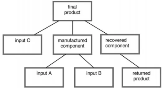
Here, we address a particular multi-stage production planning problem with remanufacturing and disposal options, and capacity constraints. Remanufacturing is understood as the industrial process of recovering items from returned products, which ensures quality and functionality as brand new manufactured items. Figure 1 shows the bill of materials (BOM) related to the particular production system here addressed.

Figure 1– Bill of materials of the production system with remanufacturing.

(5)

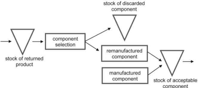
It is assumed that a known fixed average rate of units of the disassembled component, originated from units of the returned product, is not considered as input for the recovering process by not meeting the basic constitutive properties needed in the remanufacturing process, along the planning horizon. In Figure 2, we show the flow of acceptable assembling component units for the considered production planning. All the discarded items are accumulated in a tank, built specifically for this purpose, until its capacity is enough to load a garbage truck. No activities should be planned beyond the disposal.

Figure 2– Flow of acceptable assembling component units.

Also, storage capacity is considered for the stock of returned product, as well as for the stock of serviceable component and finished product. At the beginning of the planning horizon, there are no initial inventories of the items, except for the returned product, whose initial inventory level coincides with its maximal storage capacity.

A single source of external demand for the final product is considered, meaning that the market for the final product is not segmented, in the sense that customers could not differentiate a unit of the final product assembled with a brand new component from a unit assembled with a recov-ered one. (For instance, consider recovering metal hinges and handles from returned furniture, doors and gates to be used in new units of furniture, doors and gates.) The demand forecast in number of units for the final product per period is known for a coming short-term horizon. Also, independent from the demand for the final product, it is assumed that the amount of units of the returned product is known in advance for each period of the time horizon. There is no external demand for the recovered component.

3 MRP OPTIMIZATION MODEL

(6)

of the disassembled components of the returned product, as well as procuring the inputs from suppliers needed in the production processes.

The Material Requirements Planning (MRP) model integrates the decisions on the production of finished items with the decisions on the procurement of all intermediate products and raw materials to satisfy costumer demand over a short or medium-term horizon. One of the advan-tages of the MRP optimization model over the MRP decomposition approach (the one that uses spreadsheets as resources) is the opportunity to have a global optimal production plan found by an exact solution method, whereas through the decomposition version a guaranteed feasible plan can be obtained by making use of expertise and/or heuristics.

The industrial activities that should be planned in the considered production system are: purchas-ing raw materials from external suppliers, manufacturpurchas-ing units of the finished item and new units of the component, remanufacturing units of the selected returned component, and discarding use-less returned items. Procurement and production lead times, including the discarding lead time, are assumed constant along the planning horizon. They reflect the minimum time necessary for an activity to be concluded.

So, solving the MRP model will allow the determination of how much and when to procure/ produce/remanufacture/discard of each raw material/component/finished item over a short-time horizon.

Before presenting the MRP model, we show in Figure 3 the model structure based on BOM (already given in Figure 1), followed by the notation used hereafter for indices of sets, parameters and decision variables in the model.

Figure 3– Modeling structure for the production system

Indices of sets are identified as:

(7)

i =1, . . . ,6 are required as input for some other item, i =7 is the disassembled component that is discarded, i=8 is the finished item produced with new component,

i=9 is the finished item produced with remanufactured component, j ∈ D(i)representing one of the items that are direct successors of itemiin BOM.

Using these indices, we define the following deterministic parameters:

αi amount of time needed to produce one unit of itemi

βi amount of time needed to prepare the production of a batch of itemi γi procurement/manufacturing/remanufacturing/discarding lead time

for itemi

ρ average rate of assembling component units considered as inserviceable (0< ρ <1)

dt external demand for finished item in periodt, for simplicity,dt >0∀t,

hi_t unitary cost of holding in stock itemiin periodt

pi_t unitary cost of purchasing/producing/remanufacturing/discarding itemi in periodt

q_ti set-up cost of purchasing/producing/remanufacturing/discarding itemi in periodt

ri j amount of itemirequired to make one unit of item j Ct amount of returned product that is available in periodt

Kt maximum available unit capacity for remanufacturing disassembled

component in periodt

Lt maximum available time capacity for manufacturing new component and

finished item in periodt

M_ti upper bound on the units of itemithat are purchased/produced/discarded in periodt

U_ti upper bound on storage capacity of units of itemiin periodt

Vt upper bound on storage capacity of units of serviceable component in periodt.

The decision variables are:

x_ti amount of itemi purchased/produced/remanufactured/discarded in periodt y_ti indicate if itemiis purchased/produced/remanufactured/discarded or not

in periodt

s_ti amount of itemi stocked at the end of periodt

(8)

The proposed MRP model is formulated as follows:

minimize

i∈I

t∈T

pi_tx_ti +q_tiyi_t +hi_tsi_t (1)

subject to s_ti₋₁+xi

t−γi =

j∈D(i)

ri jx_tj +s_ti i =1, . . . ,6, ∀t (2)

s_ti₋₁+x_ti_−γi =s

i

t i =7, ∀t (3)

s_ti₋₁+x_ti_−γi = pd

i

t +sti i =8,9, ∀t (4)

9

i=8

pd_ti =dt ∀t (5)

x_ti ≤ M_tiy_ti ∀i, i =3,5,∀t (6)

x_ti =Ct i =3, ∀t (7)

x_ti ≤ Ktyit i =5, ∀t (8)

i

αixi_t +βiyi_t≤Lt i =6,8,9, ∀t (9)

t∈T

x_ti =ρ

t∈T

Ct

i =7 (10)

s₀i =0 ∀i, i =3 (11)

s₀i =U₀i i =3 (12)

s_ti ≤U_ti ∀i, i =5,6,∀t (13)

6

i=5

s_ti ≤Vt ∀t (14)

x∈R+I T, s∈R

I(T+1)

+ , y∈ {0,1}I T,

pd∈R2+T (15)

where the goal is to minimize the total production and inventory costs (1), and to satisfy the internal demands (2)-(3) and the non-segmented external demand (4)-(5). Although there is no demand for the discarded component, constraints (3) guarantee the flow conservation of this item. In (2) and subsequent occurrences, the notationxi

t−γi represents the amount of itemithat

(9)

availability of units of the returned product during the planning horizon. The constraint capacity on the remanufacturing and manufacturing resources is given by (8) and (9), respectively. Con-straint (10) gives the total amount of returned component that is discarded during the planning horizon, which is determined by the average rateρ. Constraints (11) assure that there are no initial inventories, except for the returned product (12), whereas constraints (13) give an upper bound to the storage of units of the items during the planning horizon, including the serviceable component (14). Decision variables are defined in (15).

Even though the amount of units of the returned product (Ct) is known in advance at the

begin-ning and for each period of the planbegin-ning horizon, it is appropriate to define a decision variable to quantify the amount of units of the returned component that is used by an optimal production plan (xt3), and consequently know the amount that is recovered (x5t), the amount that is discarded (xt7)

and stocked (s3t). This would help future strategic decisions in terms of reverse logistics, such as,

for example, augmenting the capacity of the recovering process and evaluating the costs of the recovering process. Also, condition (10) refers to disposal decisions along the planning horizon, which avoids the execution of the disposal activity every single period, whenever possible.

3.1 Problem and computational complexity

The proposed MRP model has I +(I +17)T +1 functional constraints and I +(3I +2)T variables, resulting in a problem complexity of O(I T)×O(I T). Optimization problems that are modeled as the proposed MRP are in the class of mixed integer programming (MIP).

Consider the basic MRP model as given, for example, in Pochet & Wolsey (2006). Using the notation already defined, it is formulated as follows

minimize

i∈I

t∈T

pi_tx_ti+q_tiy_ti+hi_ts_ti (16)

subject to s_ti₋₁+xi

t−γi =dti +

j∈D(i)

ri jx_tj +si_t ∀i, ∀t (17)

xi_t ≤M_tiy_ti ∀i, ∀t (18)

i

αikx_ti+βikyi_t ≤ Lk_t ∀k, ∀t (19)

x∈R+I T, s∈R

I(T+1)

+ , y∈ {0,1}I T. (20)

(10)

addressed in this work is NP-hard. (Note that we can always set to zero the parameters of the additional constraints of the model (1)-(15) to get model (16)-(20).)

4 COMPUTATIONAL EXPERIMENTS

In this section, we report computational experiments with the proposed MRP model. To this end, an arranged instance of the studied production planning problem was tested using the solver CPLEX 12.3 with the standard choice for solving mixed integer programming problems, in the software package AIMMS version 3.12. In this CPLEX version, the solution method for mixed integer linear programming problems is the branch-and-cut algorithm.

The first computational test considers the following arranged parameter selection:

α=(0,0,0,0,0,30,0,20,20); β=(0,0,0,0,0,90,0,60,60);

γ =(1,1,0,1,1,1,1,1,1); ρ=0.25; d =(10,13,16,14,15);

h =(1,2,2,1,3,3,3,5,5)∀t; p=(2,1,0,5,10,16,5,20,20)∀t;

q =(20,10,0,50,200,200,150,220,220)∀t;

r16 =2, r26 =1, r35=1, r37 =1, r48 =2, r49 =2, r59=1, r68 =1;

C =(10,8,10,8,8); Kt =20∀t; Lt =2200∀t; Mti =100∀i,∀t; Uti =30∀i,∀t,

and U₀3=30; Vt =30∀t.

Observe that the demand for the final product (d) is given for 5 periods ahead. But, to procure the needed inputs and process some production activities in advance, so that the demand for the final product in periodt =1 is satisfied, at least two periods should be anticipated, totalizing the planing horizon of at least 7 periods ahead (T = 7). Recall that the lead time is at most 1 period long.

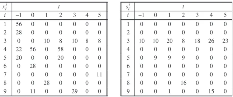
The corresponding optimal production plan is described in Table 1, and the main information from the final report generated by CPLEX is showed in Table 2. It can be observed that many of the production activities have to be anticipated so that the demand for the final product could be satisfied in each corresponding period. For example, take the demand for the final product att =1,d1 =10, as the lead time for assembling the final product with recovered component

isγ9 = 1, this activity had to be anticipated, as we observe thatx9₀ = 10, to get the optimal total cost.

4.1 Possible scenarios

(11)

Table 1– Optimal values forxi_t ands_tiof Test 1 – Given instance.

x_ti t

i –1 0 1 2 3 4 5

1 56 0 0 0 0 0 0

2 28 0 0 0 0 0 0

3 0 0 10 8 10 8 8

4 22 56 0 58 0 0 0

5 20 0 0 20 0 0 0

6 0 28 0 0 0 0 0

7 0 0 0 0 0 0 11

8 0 0 28 0 0 0 0

9 0 11 0 0 29 0 0

s_ti t

i –1 0 1 2 3 4 5

1 0 0 0 0 0 0 0

2 0 0 0 0 0 0 0

3 10 10 20 8 18 26 23

4 0 0 0 0 0 0 0

5 0 9 9 9 0 0 0

6 0 0 0 0 0 0 0

7 0 0 0 0 0 0 0

8 0 0 0 16 0 0 0

9 0 0 1 0 0 15 0

Table 2– Final Report for Test 1 – Given instance.

optimal function value 5144 number of functional constraints 198 number of real variables 140 number of integer variables 56 running time (s) 0.09 number of iterations 501 number of generated nodes 41

procurement of input A is 18, for input B is 10, and for input C is 28. The corresponding optimal production plan is described in Table 3, and the main information from the final report generated by CPLEX is showed in Table 4.

Table 3– Optimal values forx_ti andsi_t of Test 2 – Scenario 1.

xi_t t

i –1 0 1 2 3 4 5

1 4 18 0 0 0 0 0

2 1 10 0 0 0 0 0

3 0 0 10 8 10 8 8

4 28 28 24 28 28 0 0

5 10 18 0 14 15 0 0

6 0 0 11 0 0 0 0

7 0 0 0 0 0 0 11

8 0 0 0 11 0 0 0

9 0 10 18 0 14 15 0

s_ti t

i –1 0 1 2 3 4 5

1 0 4 0 0 0 0 0

2 0 1 0 0 0 0 0

3 20 2 12 6 1 9 6

4 0 8 0 2 2 0 0

5 0 0 0 0 0 0 0

6 0 0 0 0 0 0 0

7 0 0 0 0 0 0 0

8 0 0 0 0 0 0 0

(12)

Table 4– Final Report for Test 2 – Scenario 1.

The second analyzed scenario considers a maximal amount of 10 units of the finished item that can be assembled with the recovered component. This situation can occur, when resources of the recovering line is limited, due to temporary and casual events. In this case, we introduce the fol-lowing constraint into the model and consider the instance parameters of the first computational test: x_t9 ≤ 10∀t. The corresponding optimal production plan is described in Table 5, and the main information from the final report generated by CPLEX is showed in Table 6.

Table 5– Optimal values forx_ti ands_tiof Test 3 – Scenario 2.

x_ti t

i –1 0 1 2 3 4 5

1 56 0 0 0 0 0 0

2 28 0 0 0 0 0 0

3 0 0 10 8 10 8 8

4 20 76 0 40 0 0 0

5 20 0 0 20 0 0 0

6 0 28 0 0 0 0 0

7 0 0 0 0 0 0 11

8 0 0 28 0 0 0 0

9 0 10 10 0 10 10 0

s_ti t

i –1 0 1 2 3 4 5

1 0 0 0 0 0 0 0

2 0 0 0 0 0 0 0

3 10 10 20 8 18 26 23

4 0 0 0 0 20 0 0

5 0 10 0 0 10 0 0

6 0 0 0 0 0 0 0

7 0 0 0 0 0 0 0

8 0 0 0 25 9 5 0

9 0 0 0 0 0 0 0

(13)

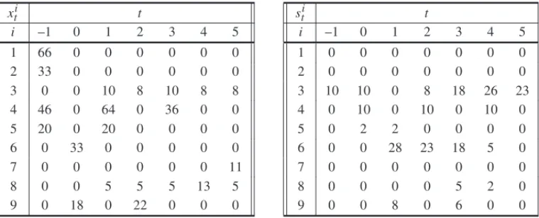
The third analyzed scenario considers that, among the units of finished item that are demanded per each period of the planning horizon, 5 units is the minimal amount that should be assembled with new manufactured component. This scenario could be generated by a client that is not confident on the recovering process. In this case, we introduce the following constraint into the model and consider also the instance parameters of the first computational test:x_t8≥5∀t. The corresponding optimal production plan is described in Table 7, and the main information from the final report generated by CPLEX is showed in Table 8.

Table 7– Optimal values forx_ti andsi_t of Test 4 – Scenario 3.

xi_t t

i –1 0 1 2 3 4 5

1 66 0 0 0 0 0 0

2 33 0 0 0 0 0 0

3 0 0 10 8 10 8 8

4 46 0 64 0 36 0 0

5 20 0 20 0 0 0 0

6 0 33 0 0 0 0 0

7 0 0 0 0 0 0 11

8 0 0 5 5 5 13 5

9 0 18 0 22 0 0 0

s_ti t

i –1 0 1 2 3 4 5

1 0 0 0 0 0 0 0

2 0 0 0 0 0 0 0

3 10 10 0 8 18 26 23

4 0 10 0 10 0 10 0

5 0 2 2 0 0 0 0

6 0 0 28 23 18 5 0

7 0 0 0 0 0 0 0

8 0 0 0 0 5 2 0

9 0 0 8 0 6 0 0

(14)

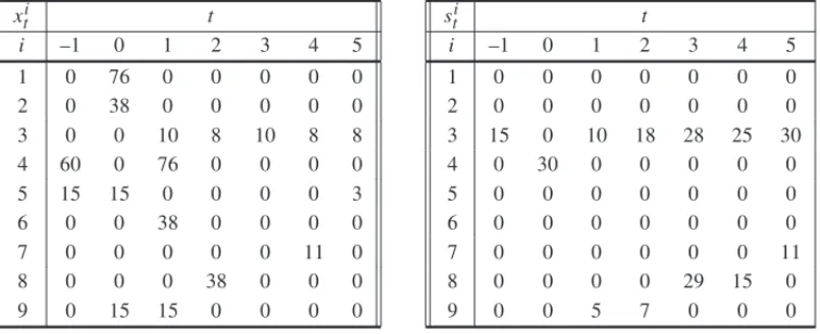
Table 9– Optimal values forx_ti ands_tiof Test 5 – Scenario 4.

x_ti t

i –1 0 1 2 3 4 5

1 0 76 0 0 0 0 0

2 0 38 0 0 0 0 0

3 0 0 10 8 10 8 8

4 60 0 76 0 0 0 0

5 15 15 0 0 0 0 3

6 0 0 38 0 0 0 0

7 0 0 0 0 0 11 0

8 0 0 0 38 0 0 0

9 0 15 15 0 0 0 0

si_t t

i –1 0 1 2 3 4 5

1 0 0 0 0 0 0 0

2 0 0 0 0 0 0 0

3 15 0 10 18 28 25 30

4 0 30 0 0 0 0 0

5 0 0 0 0 0 0 0

6 0 0 0 0 0 0 0

7 0 0 0 0 0 0 11

8 0 0 0 0 29 15 0

9 0 0 5 7 0 0 0

4.2 Computational analysis

Let us now go back to the given instance to show some analysis of the computational tests with respect to the modification of some parameters values. First, consider the variation on the data forρ, the average rate of disassembled component units considered as inserviceable, showed in Table 11.

Table 11– The optimal total costs in relation to the modification ofρ.

ρ optimal function

value 0.10 5124.2

0.25* 5144

0.50 5177

0.75 5210

(15)

From Table 11, we verify that the optimal total costs decrease when we reduce the value ofρ (ρ=0.10) from its original value (ρ =0.25). Since the disposal activities are reduced the cost of these activities is lowered, which is reflected in the optimal total costs. When we increase the value ofρ (ρ=0.50,075) from its original value (ρ =0.25), we verify that the corresponding optimal costs also increase, due to the fact that more disposal activities are processed and the inventory level of inserviceable component is larger along the planning period.

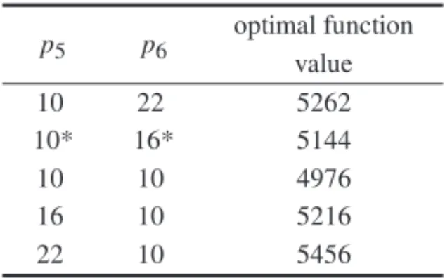
Consider now the modification on the values of the unitary manufacturing cost (p6) and the

unitary recovering cost (p5) of the main component. Recall that in the given instance the values

of the unitary manufacturing cost of the final product with new or recovered component are equal (p8=p9). The obtained optimal function values are reported in Table 12.

Table 12– The optimal total costs in rela-tion to modificarela-tion ofp5andp6.

p5 p6

optimal function value

10 22 5262

10* 16* 5144

10 10 4976

16 10 5216

22 10 5456

*indicates the original value

In relation to the given instance data, p5=10 and p6 =16, we observe that it is preferable to

assemble the finished product with recovered component than manufactured component. From Table 12, we verify that, for setting p5 = 10 and increasing p6 = 10,16,22, we get larger

optimal function values. When p6 = 10 is fixed and p5 = 10,16,22 increases, we get also

larger optimal function values. For all cases showed in Table 12, the total units of recovered component is 40 and of the manufactured component is 28 along the planning period, matching the amounts obtained for the given instance, except for the case p5 =10 and p6 =22, where

the total units of recovered component is 55 and of the manufactured component is 13.

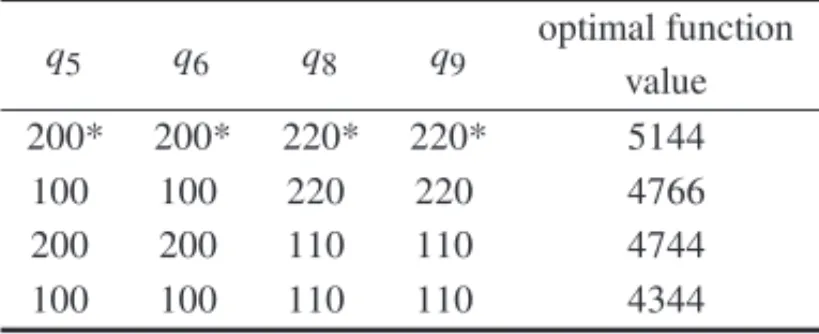
Consider now the variation of the setup costs data for the items 5 and 6 (recovered and manufac-tured component, resp.) and the items 8 and 9 (finished product with manufacmanufac-tured and recovered component, resp.) that could influence the optimal function value, as presented in Table 13.

From Table 13, we verify that reducing the setup costs causes a decreasing of the optimal function values. In particular, we verify that, halvingq5andq6, the decisions on the quantities to produce,

along the planning period, of the finished product with recovered component change from 40 to 48, whereas the quantities of the finished product with manufactured component change from 28 to 20, meaning that it is still preferable to assemble finished product with recovered component. We could see that, when the values ofq8andq9are half of their original values, the total units of

(16)

Table 13– The optimal total costs in relation to modifi-cation ofq₅,q₆,q₈, andq₉.

q5 q6 q8 q9

optimal function value 200* 200* 220* 220* 5144

100 100 220 220 4766

200 200 110 110 4744

100 100 110 110 4344

*indicates the original value

units of the finished product assembled with manufactured component changes from 28 to 13, which shows also a preference to assemble finished product with recovered component. In case q5,q6,q8, andq9are reduced in half in respect to their original values, we get the same result for

the amount of the finished product as whenq8andq9are reduced in half.

We also analyzed the sensitivity of the optimal function value for the given instance in relation to the variation of Lt, (originally set to 2200). We verified that for 1400 ≤ Lt ≤ 2200, the

optimal function value does not chance, with some differences on the inventory decisions along the planning period. The computational efforts do change; forLt = 1600, the solver finds the

solution with minimal generated nodes (12) and minimal number of iterations (297), whereas for Lt =2200, the solver finds the solution with 41 generated nodes and 501 iterations, as we can

see in Table 2.

The same analysis was performed with respect to the value ofUt, fort = 0, originally set to

Ut = 30. For 26 ≤ Ut ≤ 30, the optimal function value does not change, but the inventory

decisions do change along the planning period.

5 CONCLUSION AND FINAL COMMENTS

This work deals with the use of a technique of Operations Research to support decisions of industrial organizations that practice reverse logistics in their production systems. Specifically, a mixed integer linear programming model is proposed for the planning of materials requirements (MRP) of a particular production system with recovering and discarding process.

(17)

The optimal production plan generated with CPLEX solver would help the decision makers to decide how much and when to procure/produce/remanufacture/discard of each item involved in the production system during a time horizon. Complex production systems with remanufacturing can be easily derived from the particular production system presented here.

ACKNOWLEDGMENTS

The authors are thankful for the valuable suggestions given by the anonymous referees that im-proved the paper. The first author was partially supported by FAPERJ/CNPq through PRONEX 662199/2010-12 and CNPq Grant 311165/2013-3, whereas the last author was supported by Edital Universal 14/2012, n. 475245/2012-1.

REFERENCES

[1] BARBA-GUTIERREZ´ Y, ADENSO-D´IAZB & GUPTA SM. 2008. Lot sizing in reverse MRP for scheduling disassembly.International Journal of Production Economics,111(2): 741–751.

[2] BAYINDIRZP, ERKIPBN & G ¨ULLUB¨ R. 2007. Assessing the benefits of remanufacturing option under one-way substitution and capacity constraint.Computers & Operations Research,34: 487– 514.

[3] BITRANGR & YANASSEHH. 1982. Computational complexity of the capacitated lot size problem.

Management Science,28(10): 1174–1186.

[4] BRITOMP, DEKKERR & FLAPPERSDP. 2005. Reverse Logistics: A Review of Case Studies. In Distribution Logistics: Advanced Solutions To Practical Problems, Lecture Notes in Economics and Mathematical Systems, Bernhard Fleischmann, Andreas Klose Editors.544: 243–272, Springer.

[5] DEPUYGW, USHERJS, WALKERRL & TAYLORGD. 2007. Production planning for remanufac-tured products.Production Planning & Control: The Management of Operations,18(7): 573–583. DOI: 10.1080/0953728070154221.

[6] FLEISCHMANNM. 2000. Quantitative Models for Reverse Logistics. PhD thesis, Erasmus University Rotterdam, the Netherlands.

[7] GAREYMR & JOHNSONDS. 1979. Computers and Intractability: A Guide to NP-Completeness, Freeman.

[8] GOTZELC & INDERFURTHK. 2002. Performance of MRP in Product Recovery Systems with De-mand, Return and Leadtime Uncertainties. In Quantitative Approaches to Distribution Logistics and Supply Chain Management, Lecture Notes in Economics and Mathematical Systems,519: 99–114, Springer.

[9] HELMRICHMJR, JANSR, HEUVELWVD& WAGELMANSAPM. 2014. Economic lot-sizing with remanufacturing: complexity and efficient formulations.IIE Transactions, Special Issue: Scheduling & Logistics,46(1).

(18)

[11] KARMARKARUS & NAMBIMADOMRS. 1996. Material Allocation in MRP with Tardiness Penal-ties.Journal of Global Optimization,9: 453–482.

[12] LAGEJUNIORM & GODINHOFILHOM. 2012. Production planning and control for remanufactur-ing: literature review and analysis.Production Planning & Control,23(6): 419–435.

[13] MITRAS. 2012. Inventory management in a two-echelon closed-loop supply chain with correlated demands and returns.Computers & Industrial Engineering,62: 870–879.

[14] PAPERINDUSTRYASSOCIATIONCOUNCIL OFUSA. 2013. Paper & Paperboard Recovery. Avail-able at www.paperrecycles.org/stat pages/recovery rate.html.

[15] PINEYRO˜ P & VIERAO. 2010. The economic lot-sizing problem with remanufacturing and one-way substitution.International Journal of Production Economics,124(2): 482–488.

[16] PINEYRO˜ P & VIERA O. 2012. Analysis of the quantities of the remanufacturing plan of perfect cost. Journal of Remanufacturing, 2(3). Available at: http://www.journalofremanufacturing.com/ content/2/1/3.

[17] POCHETY & WOLSEYLA. 2006. Production Planning by Mixed Integer Programming. Springer Series in Operations Research and Financial Engineering, Springer.

[18] REIMANNM & ZHANGW. 2013. Joint optimization of new production, warranty servicing strategy and secondary market supply under consumer returns.Pesquisa Operacional,33(3), Rio de Janeiro, Setp/Dec 2013.

[19] ROGERSDS & TIBBEN-LEMBKERS. 1999. Going backwards: reverse logistics trends and prac-tices. University of Nevada, Reno, Center for Logistics Management, Reverse Logistics Executive Council.

[20] SCHULZT & FERRETTII. 2011. On the alignment of lot sizing decisions in a remanufacturing system in the presence of random yield.Journal of Remanufacturing,1(3). DOI:10.1186/2210-4690-1-3.

[21] SRIVASTAVASK. 2008. Network design for reverse logistics.Omega,36: 535–548.

[22] TEUNTERR. 2004. Lot-sizing for inventory systems with product recovery.Computers & Industrial Engineering,46: 431–441.

[23] THIERRYM, SALOMONM, VANNUNENJ & VANWASSENHOVELN. 1995. Strategic issues in