Braz. J. Chem. Eng. vol.29 número1

ISSN 0104-6632 Printed in Brazil

www.abeq.org.br/bjche

Vol. 29, No. 01, pp. 183 - 201, January - March, 2012

*To whom correspondence should be addressed

Brazilian Journal

of Chemical

Engineering

DEVELOPMENT OF A HIGH-ORDER FINITE

VOLUME METHOD WITH MULTIBLOCK

PARTITION TECHNIQUES

E. M. Lemos, A. R. Secchi

*

and E. C. Biscaia Jr.

PEQ/COPPE, Federal University of Rio de Janeiro, CT, Rio de Janeiro - RJ, Brazil. Universidade Federal do Rio de Janeiro, Instituto Alberto Luiz Coimbra de Pós Graduação e Pesquisa de Engenharia, Av. Horácio Macedo 2030, Centro de Tecnologia, Bloco G, Sala G-116,

Cidade Universitária, Fundão, C. P. 68502, CEP: 21941-914, Rio de Janeiro, RJ - Brasil. E-mail: arge@peq.coppe.ufrj.br

(Submitted: June 23, 2011 ; Revised: September 14, 2011 ; Accepted: November 6, 2011)

Abstract - This work deals with a new numerical methodology to solve the Navier-Stokes equations based on a finite volume method applied to structured meshes with co-located grids. High-order schemes used to approximate advective, diffusive and non-linear terms, connected with multiblock partition techniques, are the main contributions of this paper. Combination of these two techniques resulted in a computer code that involves high accuracy due the high-order schemes and great flexibility to generate locally refined meshes based on the multiblock approach. This computer code has been able to obtain results with higher or equal accuracy in comparison with results obtained using classical procedures, with considerably less computational effort.

Keywords: Finite volume method; Navier-Stokes; High-order interpolation schemes; Multiblock partition techniques.

INTRODUCTION

Using computational fluid dynamics (CFD) in a safe and reliable way must attend to several prerequisites, such as the development of a mathematical model able to describe the process under consideration and the application of appropriate numerical tools to solve the proposed model. Mechanistic modeling includes mass, energy, and momentum conservation laws, coupled with state and constitutive equations. A great number of methodologies have been applied to solve these equations, the most popular are: Finite Difference Methods (FDM), Finite Element Methods (FEM) and Finite Volume Methods (FVM) (Hirsch, 2007).

The FVM is currently the most common method used to solve fluid flow problems (Cebeci et al., 2005). This popularity is directly related to its

conservative nature, since in flow simulations it is extremely important to satisfy the conservation laws at all levels, avoiding generation/consumption of mass, energy, or momentum due to artificial terms inside the control volume, independent of the mesh size. The same is not guaranteed in finite difference and finite element methods.

Brazilian Journal of Chemical Engineering

Low order interpolation schemes can lead to inaccurate results provoked by numerical diffusion effects (Hirsch, 2007; Patankar, 1980; Versteeg and Malalasekera, 2007).

Alternatively, high-order interpolation schemes produce more accurate solutions with low computational costs (Muniz et al., 2008; Piller and Stalio, 2004; Leonard, 1995). However, to maintain the global order of the approximation, it is important that all approximation formulas for the advective, diffusive and nonlinear terms have the same order of accuracy (Leonard, 1995).

When applying high-order schemes to nonuniform meshes, it is necessary to keep in mind several precautions in the development of interpolation formulas, since interpolation schemes were originally developed for uniform meshes (Lacor et al., 2004).

Multiblock treatment allows mesh refinement in selected regions of the problem domain that should not be necessarily extended to other regions. This is a desirable characteristic of mesh refinement techniques, making the multiblock treatment a more efficient procedure in comparison with single block techniques, especially when applied to complex geometries problems (Farrashkhalvat and Miles, 2003; Serón and Sabadell, 2000). Interconnection between adjacent blocks with different degrees of mesh refinement, avoiding loss of accuracy and/or creation of discontinuities, is the main challenge in computer implementation of multiblock procedures (Serón and Sabadell, 2000; Berger, 1987; Liu and Shyy, 1996; Chen et al., 1997).

The development of a high-order finite volume method and a multiblock partition technique of the problem domain to solve the Navier-Stokes equations are the main objectives of this paper, as described in Sections 3 and 4, respectively. This new procedure applies the basic principles of the finite volume method (FVM) using structured meshes and co-located grids of problem variables, described in the next section. The combination of these two techniques resulted in the development of a computer code that associates the better accuracy of higher-order schemes with the greater flexibility of the multiblock treatment. This code was capable of solving several benchmarks problems like the ones presented in Section 5, with low computational costs in comparison with traditional procedures.

MATHEMATICAL MODEL AND APPLICATION OF THE FINITE VOLUME METHOD

In order to illustrate the proposed numerical procedure to solve the Navier-Stokes equations, the stationary and isothermal flow of an incompressible Newtonian fluid was considered and modeled by mass and momentum conservation equations, presented below in a dimensionless form:

( )

*

0

∇ ⋅ v = (1)

( )

* * * 2 *

Re⎡_⎣∇ ⋅ v v ⎤_⎦= −∇ + ∇p v (2)

where v*=v/ v₀ represents the dimensionless velocity vector, p*=p / vρ 2₀ the dimensionless pressure, Re= ρv L /_{0 0} μ the Reynolds number, μ the Newtonian viscosity, ρ the density, L and ₀ v ₀ the characteristic length and velocity of the problem, respectively.

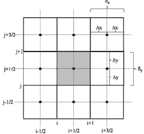
The application of FVM consists basically of subdividing the problem domain into elementary control volumes, as illustrated in Figure 1, and integrating each of those partial differential equations in these volumes, resulting in a nonlinear algebraic system, composed, in the two-dimensional case, by the equations presented below:

Figure 1: Representation of the control volume.

( )

y

( )

y

( )

x

( )

x

x ₁ x ₁ y ₁ y ₁

i 1, j i, j i , j 1 i , j

2 2 2 2

v v y v v x 0

+ + + + + +

⎡ ⎤ ⎡ ⎤

⎢ ₋ ⎥_{Δ +}⎢ ₋ ⎥_{Δ =}

⎢ ⎥ ⎢ ⎥

 

Brazilian Journal of Chemical Engineering Vol. 29, No. 01, pp. 183 - 201, January - March, 2012

( )

( )

( )

( )

( )

( )

y y x x

x x ₁ x x ₁ y x ₁ y x ₁

i 1, j i, j i , j 1 i , j

2 2 2 2

y y

y y x x

1 1

i 1, j i, j _{1 1}

2 2 i 1, j i, j

2 2

Re v v v v y v v v v x

v v

p p y y

x x

+ + + + + +

+ + +

+ + +

⎡⎡ ⎤ ⎡ ⎤ ⎤

⎢⎢ − ⎥Δ +⎢ − ⎥Δ =⎥

⎢⎢_⎣ ⎥_⎦ ⎢_⎣ ⎥_⎦ ⎥

⎣ ⎦

⎡ ⎤

⎡ ⎤ _⎢⎛_∂ ⎞ ⎛_∂ ⎞ _⎥

⎢ ⎥ ⎜ ⎟ ⎜ ⎟

− − Δ +_⎢ − _⎥Δ

⎜ ∂ ⎟ ⎜ ∂ ⎟

⎢ ⎥ _{⎢⎝ ⎠ ⎝ ⎠ ⎥}

⎣ ⎦ _{⎢⎣ ⎥⎦}

(4)

( )

( )

( )

( )

( )

( )

y y x x

x y ₁ x y ₁ y y ₁ y y ₁

i 1, j i, j i , j 1 i , j

2 2 2 2

y y

y y

x x

1 1

i , j 1 i , j _{1 1}

2 2 _{i 1, j i, j}

2 2

Re v v v v y v v v v x

v v

p p x y

x x

+ + + + + +

+ + +

+ + +

⎡⎡ ⎤ ⎡ ⎤ ⎤

⎢⎢ − ⎥Δ +⎢ − ⎥Δ =⎥

⎢⎢_⎣ ⎥_⎦ ⎢_⎣ ⎥_⎦ ⎥

⎣ ⎦

⎡ ⎤

⎡ ⎤ ⎢⎛_∂ ⎞ ⎛_∂ ⎞ ⎥

⎜ ⎟ ⎜ ⎟

⎢ ⎥

− − Δ +⎢ − ⎥Δ

∂ ∂

⎜ ⎟ ⎜ ⎟

⎢ ⎥ ⎢_{⎝ ⎠ ⎝ ⎠} ⎥

⎣ ⎦ _{⎢ ⎥}

⎣ ⎦

(5)

In this contribution, a structured uniform volume was considered, i.e., the points located at the vertex of the control volume are equally spaced from the control volume center with distances ∆x and ∆y. Fractional index values represent points located at the control volume center and integer index values represent points located at the faces. The terms

( )

x 1 i , j

2

+

ϕ ,

( )

y

1 i, j

2

+

ϕ _e

( )

xy 1 1 i , j

2 2

+ +

ϕ _represent,

respectively, the average value of a property in the control volume face parallel to the x direction, the average value of a property in the control volume face parallel to the y direction, and the average value of a property in the control volume center, according to the following expressions:

( )

i 1

(

)

i

x x

1 i , j

x 2

x x , y d

+

+

ϕ Δ =

∫

ϕ + δ δ (6)

( )

j 1

(

)

j

y y

1 i, j

y 2

y x, y d

+

+

ϕ Δ =

∫

ϕ + ξ ξ (7)

( )

i 1 j 1

(

)

i j

y x xy

1 1 i , j

x y

2 2

x y x , y d d

+ +

+ +

ϕ Δ Δ =

∫ ∫

ϕ + δ + ξ δ ξ (8)

Usually, the values of the variables in each control volume face are assumed to be their corresponding values in the center of the control

volume face. Because this assumption presents an approximation order of two, its use limits the global approximation order to the same order.

In the methodology proposed in this paper, the average values of the variables are computed directly as described by Equations (3), (4) and (5), and, in a post-processing stage, nodal values of the variables are recovered through deconvolution techniques. Direct use of the average values avoids numerical approximation schemes for the integrals involved, reducing, as a consequence, the number of discretization points and making the proposed procedure faster and more accurate than conventional procedures (Muniz et al., 2008; Pereira et al., 2001). Values of the variables in each of control volume face are obtained by polynomial interpolation using values of the corresponding variable at the center of neighboring control volumes.

The discretized system of equations represented by Equations (3), (4) and (5) was solved directly by using the code DASSLC Version 3.2 (SECCHI, 2007). This code applies Newton’s method to the solution of nonlinear systems of equations, using sparse LU factorization in the solution of linear systems. As all equations are solved simultaneously, the pressure-velocity coupling is ensured.

HIGH-ORDER INTERPOLATION SCHEMES

Brazilian Journal of Chemical Engineering

meshes, hence, as a consequence reducing simulation processing time (Muniz et al., 2008; Piller and Stalio, 2004; Leonard, 1995; Kobayashi, 1999; Pereira et al., 2001). Fourth-order Lagrange interpolation schemes have been considered in this paper.

The numerical procedure was developed using the same approximation order for advective, diffusive and nonlinear terms (Leonard, 1995), considering also the same approximation order inside and at the boundaries of the domain (Kobayashi, 1999).

Average variable values at the control volume walls obtained by fourth-order Lagrange interpolation can be defined by:

( )

( )

( )

( )

( )

y xy xy

1 3 1 1 1

i, j i , j i , j

2 2 2 2 2

xy xy

1 1 3 1

i , j i , j

2 2 2 2

a b

c d

+ − + − +

+ + + +

ϕ = ϕ + ϕ +

ϕ + ϕ

(9)

To complete this approximation procedure, the coefficients are determined as follows: Step 1: Expand the variable in a Taylor series around a point (x0, y0).

Step 2: Calculate all the average values presented in Equation (9) through Taylor expansions determined in Step 1.

Step 3: Substitute all average values obtained in step 2 in Equation (9).

Step 4: Identifying terms of equal derivative order in the equation obtained in Step 3, a linear system of algebraic equations can be built and solved, where the unknowns are the coefficients of the approximation.

Step 5: In addition, it is possible to estimate the approximation error, applying the coefficients obtained in Step 4 in Equation (9), and calculating the difference between this approximation and the value obtained by Taylor series expansion.

Applying the procedure described to determine the coefficients a, b, c and d in Equation (9), the following expression was obtained.

( )

( )

( )

( )

( )

y xy xy

1 3 1 1 1

i, j i , j i , j

2 2 2 2 2

xy xy

1 1 3 1

i , j i , j

2 2 2 2

1 7

12 12

7 1

12 12

+ − + − +

+ + + +

ϕ = − ϕ + ϕ +

ϕ − ϕ

(10)

When the above expression is applied to regions near the boundaries, such as i=0, 1, N−1and N, the approximation scheme requires information related to points outside the problem domain. To avoid this

undesirable behavior, new interpolation schemes have been proposed, where only internal interpolation points are considered. The coefficients of these schemes were obtained using the same procedure described above and the results are presented in the Appendix section.

The same fourth-order Lagrange interpolation procedure has been applied to calculate diffusive terms, resulting in the following equation:

( )

( )

( )

( )

xy xy

3 1 1 1

i , j i , j

y _{2 2 2 2}

1 xy xy

i, j

1 1 3 1

2 _{i , j i , j}

2 2 2 2

1 5

12 4

1

x x _{5 1}

4 12

− + − +

+

+ + + +

⎛ _{ϕ − ϕ +}⎞

⎜ ⎟

⎛_∂ϕ ⎞ ⎜ ⎟

⎜ ⎟ = ⎜ ⎟

⎜ ∂ ⎟ _{Δ ⎜ ⎟}

⎝ ⎠ _{⎜ ϕ − ϕ ⎟}

⎜ ⎟

⎝ ⎠

(11)

Again, the above equation cannot be directly applied in regions near the boundaries. In this case, the same new interpolation scheme was applied and is detailed in the Appendix section.

Nonlinear terms are commonly founded in Navier-Stokes equations, such as products of velocity components,

v

_x

v

_x,

v

_x

v

_y and

v

_y

v

_y, normally present in momentum conservation equations. Normally the average values of these products are considered as the product of the average value of each parcel. However, this simplification limits the approximation order to two, and may cause a reduction in the global order of the approximation.

Expanding the nonlinear product term in a Taylor series, Pereira et al., (2001) concluded that the error between the average value of the product of the variables and the product of the average value of each parcel is equal to the product of the derivative of each parcel followed by a fourth-order term, as presented below:

( )

( ) ( )

( )

y y y

1 2 ₁ 1 ₁ 2 ₁

i, j i, j i, j

2 2 2

2

4

1 2

1 1

i, j i, j

2 2

y

O h

12 y y

+ + +

+ +

ϕ ϕ ≈ ϕ ϕ +

⎛ ⎞⎛ ⎞

Δ _⎜∂ϕ _⎟⎜∂ϕ _{⎟ +}

⎜ _∂ ⎟⎜ _∂ ⎟

⎜ ⎟⎜ ⎟

⎝ ⎠⎝ ⎠

(12)

Based on this expression, a fourth-order procedure was proposed to approximate the average values of variable products, adding to the product of the averages of each variable a new term involving the derivatives of these variables, as shown in the Appendix section.

 

Brazilian Journal of Chemical Engineering Vol. 29, No. 01, pp. 183 - 201, January - March, 2012

values of the coefficients a, b, c and d in the approximation formula, as given by the equation:

( )

( )

( )

( )

( )

x x

3 1

i, j

i , j i , j

2 2

x x

1 3

i , j i , j

2 2

1 7

12 12

7 1

12 12

− −

+ +

ϕ = − ϕ + ϕ +

ϕ − ϕ

(13)

Equivalent deconvolution expressions applied to boundary and near boundary node points are detailed in the Appendix section.

MULTIBLOCK CONNECTION TECHNIQUE

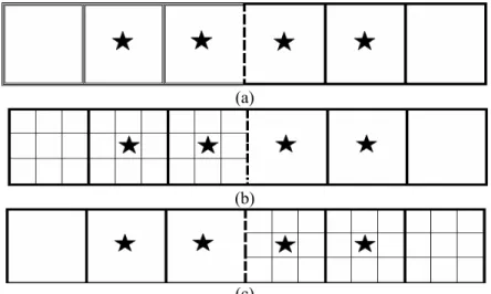
The main disadvantage of using structured grids is the inability to refine only a specific region of the problem domain without extending the refinement to other regions, Figure 2a. An alternative to revert this limitation is the application of a multiblock treatment, which consists of the partitioning of the problem domain into a determinate number of blocks or subdomains. For each one of these blocks, a different degree of refinement is allowed, refining regions of interest while using coarser grids in other regions, Figure 2b.

The partitioning of the spatial domain into subdomains implies a series of benefits such as: reduction of the numerical complexity by solving subproblems of smaller dimensions, the solution of problems in complex geometries can be obtained more efficiently in simpler subdomains, and each subdomain can be assigned to a different processing unit of a cluster, accelerating the solution procedure (Serón and Sabadell, 2000).

The different alternatives for exchanging

information between blocks are classified according to the topology and the constraints used during the mesh generation, the most widely used in the literature being: patched meshes and chimera or overlapped meshes. In the patched meshes, there is no overlap between the blocks and the only connection that exists occurs through the common frontier. In the overlapped meshes, the blocks are positioned in an overlapping structure and the information is exchanged between the blocks using interpolation functions.

Over the past decades, several techniques have been developed for generation of structured grids in complex geometries. It is generally agreed that the implementation of conservative schemes is more suitable for the faces where there are shock waves and high gradients, and most studies apply linear interpolation formulas (Berger, 1987) or bilinear interpolation formulas (Liu and Shyy, 1996; Chen et al., 1997). A block-structured local refinement method based on a conservative finite volume was applied by Barad and Colella (2005) using the classical Mehrstellen methods.

The development of a computational procedure that applies the multiblock partition technique should be able to deal efficiently with the transfer of information between blocks when connecting blocks with different degrees of refinement. Each block should be able to recognize the kind of boundary (wall, inlet, outlet, symmetry, or other block) its face is connected to. Beyond these characteristics, the connection procedure should be able to maintain the approximation order of interpolations on the interface between blocks. The maintenance of the approximation order is extremely important because the errors associated with a possible order reduction derived from the multiblock connection technique can be propagated through the domain decreasing the accuracy of the procedure.

(a) (b)

Brazilian Journal of Chemical Engineering

The technique developed for block connection with different degrees of refinement uses the fourth-order Lagrange interpolation for connecting the blocks, ensuring the maintenance of the global order of approximation. The application of this technique was only possible due to the methodology developed for mesh generation that allows the direct connection between blocks.

Recalculating the interpolation schemes by writing their coefficients as functions of the degree of mesh refinement was not able to maintain the order of accuracy of the original scheme, being reduced to a second order. Thus, for this interpolation scheme be applied, the number of interpolation points should be greater than that applied in the fourth-order Lagrange interpolation formula, which would increase the computational effort.

A better approach was to make refinements using only odd multiples for ∆x and ∆y, the length and height of the control volumes, respectively. The great advantage of this procedure is that the control volume centers of the blocks are located on the same symmetry line in the connection interface, making it possible to use the same Lagrange interpolation formula. In this approach, it was only necessary to develop a procedure that identifies the points that are located at the control volume centers of the more refined mesh located at the same distances ∆x or ∆y of the less refined mesh. From this condition, a formula was developed for block connection that

could be done in a simple and automatic way, with the fundamental requirement of maintaining the approximation order of the interpolation scheme.

In order to facilitate the computational implementation of the refinement procedure, a block refinement index (IR) was defined, relating the size of the control volumes of a block to a reference size. Multiples of three were chosen for mesh refinement, where the size of the control volumes of a block is calculated by the following expressions:

Base Block

IR

x x

3

Δ

Δ = Block Block

IR= ⇒ Δ0 x = Δx (14)

Base Block

IR

y y

3

Δ

Δ = Block Block

IR= ⇒ Δ0 y = Δy

As all the blocks that form the computational mesh are generated using multiples of ∆x and ∆y, it is possible to perform the direct connection between blocks, it only being necessary to identify the points in the neighboring meshes that have the same values of

∆x or ∆y in which the interpolation formulas must be evaluated.

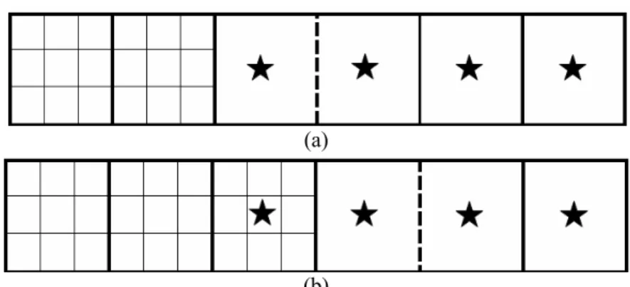
The boundary between blocks can occur in three different ways: the block refinement index is equal to (Figure 3a), less than (Figure 3b) or greater than (Figure 3c) the refinement index of its neighboring block.

Δx Δx

Δy

Δy

(a)

Δx/3 Δx

Δy

Δy/3

(b)

Δx/3

Δx

Δy

Δy/3

(c)

 

Brazilian Journal of Chemical Engineering Vol. 29, No. 01, pp. 183 - 201, January - March, 2012

Using the mesh refinement described above, the interpolation formulas applied near the interface between blocks were formulated using two points inside of the block domain and two points located in the neighboring block, as shown in Figure 4.

Because fourth-order interpolation schemes were used in this work, the points located at volume faces near the interface can also be part of multiblock connection, Figure 5, thereby increasing the amount of information transferred between blocks and improving the convergence procedure.

However, for points near the interface in which the block is more refined than the neighboring block, it is

not worthwhile to exchange information between meshes, because the use of any set of points belonging to the less-refined neighboring mesh does not result in a scheme that will be able to keep the required approximation order. For this case, it is better to apply an interpolation scheme that uses only points inside of the block domain, as shown in Figure 6.

For the points near the interface in which the block presents less refinement than the neighboring block, two approaches are possible: the first one does not consider points of the more refined mesh, Figure 7a, while the second one includes the information from the more refined mesh, Figure 7b.

(a)

(b)

(c)

Figure 4: Illustrative representation of the multiblock connection applied to meshes: (a) of equal refinement, (b) block with lower index of refinement and (c) block with higher index of refinement.

Figure 5: Illustrative representation of the points located at volume faces near to the interface that can be included in the connection between blocks.

Brazilian Journal of Chemical Engineering

(a)

(b)

Figure 7: Illustrative representation of the multiblock connection applied to meshes with lower index of refinement for points near to the interface connection using: (a) only internal points and (b) with information of the neighboring block.

The interpolation functions for approximating the advective terms according to Figures 4a, 4b, 4c, 6, 7a, and 7b, are given, respectively, by:

( )

bl

( )

blv

( )

blv

( )

bl

( )

bl

y xy xy xy xy

3 1 1 3

0, j Nx , j Nx , j , j , j

2 2 2 2

1 7 7 1

12 − 12 − 12 12

ϕ = − ϕ + ϕ + ϕ − ϕ

(15)

( )

bl

( )

blv

( )

blv

( )

bl

( )

bl

y xy xy xy xy

1 3

0, j Nx CR 2, j Nx CR1, j , j , j

2 2

1 7 7 1

12 − 12 − 12 12

ϕ = − ϕ + ϕ + ϕ − ϕ

(16)

( )

bl

( )

blv

( )

blv

( )

bl

( )

bl

y xy xy xy xy

3 1

0, j Nx , j Nx , j CR1, j CR 2, j

2 2

1 7 7 1

12 − 12 − 12 12

ϕ = − ϕ + ϕ + ϕ − ϕ

(17)

( )

bl

( )

bl

( )

bl

( )

bl

( )

bl

y xy xy xy xy

1 3 5

1, j 0, j , j , j , j

2 2 2

1 13 5 1

4 12 12 12

ϕ = ϕ + ϕ − ϕ + ϕ

(18)

( )

bl

( )

bl

( )

bl

( )

bl

( )

bl

y xy xy xy xy

1 3 5

1, j 0, j , j , j , j

2 2 2

1 13 5 1

4 12 12 12

ϕ = ϕ + ϕ − ϕ + ϕ

(19)

( )

bl

( )

blv

( )

bl

( )

bl

( )

bl

y xy xy xy xy

1 3 5

1, j Nx CR1, j , j , j , j

2 2 2

1 7 7 1

12 − 12 12 12

ϕ = − ϕ + ϕ + ϕ − ϕ

(20)

where bl refers to the block and blv refers to its neighboring block, CR1=3IR/2 and CR2=3IR+1/2.

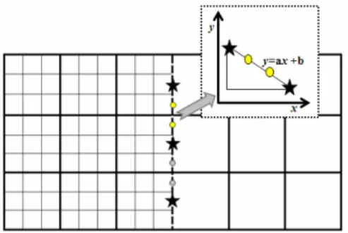
The values of the faces of the control volumes located in the mesh with greater refinement that do not present coincident control volume centers are approximated by a linear interpolation formula using the values of the mesh of the smallest refinement, as shown in Figure 8. The original fourth-order Lagrange interpolation formulas are only applied to the common

 

Brazilian Journal of Chemical Engineering Vol. 29, No. 01, pp. 183 - 201, January - March, 2012

Figure 8: Schematic representation of the

interpolation procedure for mesh of higher degree of refinement.

The interpolation formulas in Equations (15) to (20) were applied to the left face of the block, and similar formulas were also developed for the top, bottom and right faces, as well as for the other linear and nonlinear terms, not presented here.

Although only the fourth-order Lagrange interpolation scheme (LAG4) has been used in this work, the procedure developed for multiblock connection can be extended to schemes with higher or lower orders.

RESULTS

Examples from the literature, commonly used for testing and evaluation of numerical procedures, were considered for evaluation of the higher-order technique with multiblock treatment proposed in this work. The examples used were: the flow between parallel plates preceded by a free-slip surface (slip-stick), the outlet flow between parallel plates for a free-slip surface (stick-slip), and the flow in a square cavity under the action of a sliding plate (lid-driven).

Slip-Stick Flow

This problem consists of a fluid flow between two plane and parallel plates. Initially, the flow happens on a free-slip surface and is followed by a non-slip condition applied on the plate surface, Figure 9. The main feature of this problem is the presence of singularity when the boundary conditions changes from the free-slip condition to the no-slip condition.

Figure 9: Schematic representation of slip-stick flow.

Since the problem is symmetric along the x-axis, it is possible to reduce the size of the computational grid, using the symmetry condition at the central horizontal section, simulating in this way only half of the initial domain. As input condition, a constant velocity profile was applied, for a Reynolds number of 10. In the output, the pressure was specified as zero and the established flow condition was considered. The length of the plate before the singularity is L1=3 and after the singularity is L2=7 and the plate half height is H=1. The dimensionless positions x and y are taken from the point where the horizontal line of symmetry (y=0) and the beginning of the flow (x=0) are located.

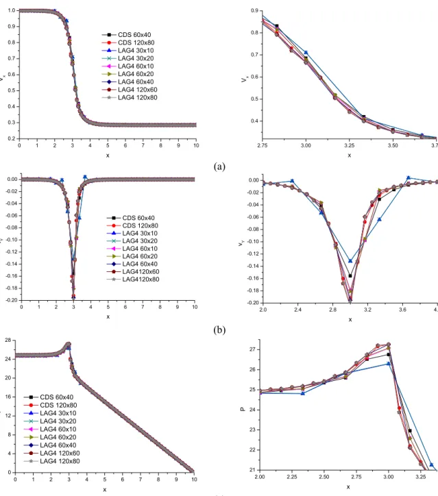
The profiles presented in Figure 10 compare the results for the horizontal line y=0.9 obtained by the LAG4 scheme using different mesh refinements with the results obtained by the central differences scheme (CDS) using 60x40 and 120x80 meshes.

Comparing the profiles presented in Figure 10, it can be seen that the solution using the LAG4 procedure with the 60x40 mesh presents a similar result to the 120x80 mesh indicating a converged mesh. The result obtained by the LAG4 scheme using the 60x40 mesh presents a solution similar to the solution obtained by the CDS scheme using the 120x80 mesh, showing the advantage of a higher order scheme. The most significant differences are observed only for the velocity profile vy, Figure 10b, with the presence of overshoot in the numerical solution obtained by the LAG4 scheme using the 30x10 and 30x20 meshes, which is characteristic of the application of high-order approximations. This problem can be minimized by increasing the computational mesh refinement, as can be observed for the 60x10, 60x20, 60x40, 120x60 and 120x80 meshes, where these oscillations no longer occur.

Comparing the computational time to find solutions with the same degree of accuracy, using a computer with a 3.20 GHz Intel i5 processor with 8.0 GB of memory, it is possible to observe the better performance of the LAG4 scheme, where the application of a 60x40 mesh spent 480 seconds to obtain the solution, while the CDS scheme with the application of a 120x80 mesh spent 1135 seconds. These results clearly demonstrate the superiority of the higher-order schemes.

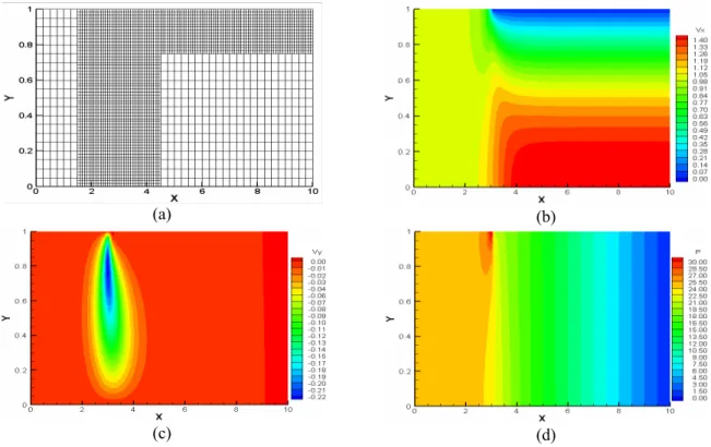
Figure 11 presents the velocity and pressure contour plots obtained by the application of the multiblock partition technique to the problem. In this case, the mesh was only refined in the required regions, i.e., near the singularity and the wall, as shown in Figure 11a, resulting in a mesh composed of 3600 control volumes.

Brazilian Journal of Chemical Engineering

in the region near the singularity for all the domain, resulting in the 120x60 mesh. Figure 12 compares the profiles of horizontal velocity vy at different y cuts and Table 1 shows the root mean square difference between the solutions, where it is possible to observe that there are no significant discrepancies between the obtained solutions.

It is important to note that the computational effort for the multiblock procedure is much less than

the full refinement, because in the latter 7200 control volumes were used, while only 3600 control volumes were necessary for the multiblock. This considerable reduction of the mesh size decreases the computational time from 1770 seconds for the full refinement to 851 seconds for the multiblock procedure without compromising the quality of the solution, clearly demonstrating the advantage of using a block structured mesh.

0 1 2 3 4 5 6 7 8 9 10

0.2 0.3 0.4 0.5 0.6 0.7 0.8 0.9 1.0

CDS 60x40 CDS 120x80 LAG4 30x10 LAG4 30x20 LAG4 60x10 LAG4 60x20 LAG4 60x40 LAG4 120x60 LAG4 120x80

Vx

x

2.75 3.00 3.25 3.50 3.75

0.4 0.5 0.6 0.7 0.8 0.9

Vx

x (a)

0 1 2 3 4 5 6 7 8 9 10

-0.20 -0.18 -0.16 -0.14 -0.12 -0.10 -0.08 -0.06 -0.04 -0.02 0.00

CDS 60x40 CDS 120x80 LAG4 30x10 LAG4 30x20 LAG4 60x10 LAG4 60x20 LAG4 60x40 LAG4120x60 LAG4120x80

vY

x

2.0 2.4 2.8 3.2 3.6 4.0

-0.20 -0.18 -0.16 -0.14 -0.12 -0.10 -0.08 -0.06 -0.04 -0.02 0.00

vY

x (b)

0 1 2 3 4 5 6 7 8 9 10

0 4 8 12 16 20 24 28

CDS 60x40 CDS 120x80 LAG4 30x10 LAG4 30x20 LAG4 60x10 LAG4 60x20 LAG4 60x40 LAG4 120x60 LAG4 120x80

P

x

2.00 2.25 2.50 2.75 3.00 3.25 21

22 23 24 25 26 27

P

x (c)

 

Brazilian Journal of Chemical Engineering Vol. 29, No. 01, pp. 183 - 201, January - March, 2012

(a) _(b)

(c) (d)

Figure 11: Contour plots obtained for the slip-stick flow using the multiblock procedure: (a) Mesh; (b) Contour plot for velocity vx; (c) Contour plot for velocity vy and (d) Contour plot for pressure.

0 1 2 3 4 5 6 7 8 9 10

-0.22 -0.20 -0.18 -0.16 -0.14 -0.12 -0.10 -0.08 -0.06 -0.04 -0.02 0.00

Vy

x

y=0.1 y=0.3 y=0.5 y=0.7 y=0.9

y=0.1 y=0.3 y=0.5 y=0.7 y=0.9

0 1 2 3 4 5 6

-0.08 -0.07 -0.06 -0.05 -0.04 -0.03 -0.02 -0.01 0.00

Vy

x

y=0.1 y=0.3 y=0.5 y=0.7 y=0.9

y=0.1 y=0.3 y=0.5 y=0.7 y=0.9

Figure 12: Comparison between the velocity profiles vy for different y cuts using the homogeneous refined 120x60 mesh (represented by lines) and multiblock mesh (represented by dots).

Table 1: Normalized difference between the solutions obtained by application of the multiblock technique and the solutions obtained using the homogeneous degree of refinement for the slip-stick flow.

ref x x

ref x

v - v

v

ref y y

ref y

v - v

v

ref

ref

p - p

p

y=0.1 3.6786×10-4 2.1848×10-4 2.0658×10-3

y=0.3 2.0745×10-4 _7.7912×10-4 _4.5808×10-3

y=0.5 7.8678×10-4 1.5522×10-4 5.2507×10-3

y=0.7 7.3347×10-4 1.6401×10-4 2.3105×10-3

Brazilian Journal of Chemical Engineering Lid-Driven Flow

The flow in a square cavity consists of a liquid initially at rest, which has the upper surface of the cavity in contact with a sliding plate that moves with constant velocity V, Figure 13. For this example two flow conditions are studied: the first considering the Reynolds number of 100 and the second considering the Reynolds number of 400.

Figure 13: Schematic representation of lid-driven flow. Table 2 presents the results for Re=100 obtained by Botella and Peyret (1998) using a spectral method with Chebyshev collocation, Deng et al. (1994)

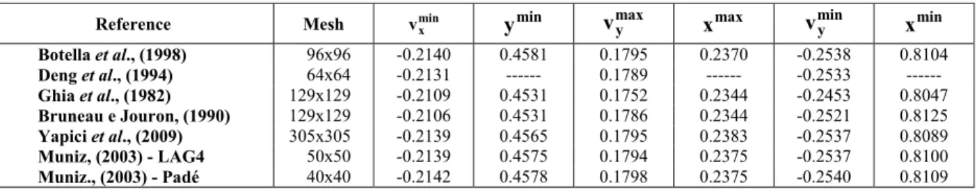
using FVM with Richardson extrapolation, Ghia et al. (1982) and Bruneau and Jouron (1990) using the finite difference method with multigrid technique, Yapici et al., (2009) using FVM with CDS scheme, and Muniz et al. (2003) using FVM with fourth-order Lagrange and Padé interpolation schemes. The values of the minimum speed vx, taken at the vertical center line (x=0.5), followed by the corresponding y value and also the values of the maximum and minimum velocity vy in the central horizontal line (y=0.5) followed by the corresponding x values, are presented. Table 3 shows the values of minimum and maximum velocities at x=0.5 and y=0.5 obtained in this work using the LAG4 scheme with different mesh refinements.

Comparing the results obtained by the LAG4 scheme with the results taken from the literature, Table 3, it is possible to observe a good agreement between the results obtained. It is important to highlight the degree of accuracy obtained by the LAG4 scheme, that, even using meshes with a lower degree of refinement, was able to obtain satisfactory solutions, especially when comparing the results of Ghia et al. (1982) and Bruneau and Jouron (1990) using a 129x129 mesh with the results of LAG4 using a 20x20 mesh, and the results of Yapici et al., (2009) using a 305x305 mesh with the results of LAG4 using a 60x60 mesh.

Table 2: Values of the minimum and maximum velocities at x=0.5 and y=0.5 for the lid-driven problem from the literature for Re=100.

Reference Mesh vminx ymin

max y

v max

x vminy xmin

Botella et al., (1998) 96x96 -0.2140 0.4581 0.1795 0.2370 -0.2538 0.8104

Deng et al., (1994) 64x64 -0.2131 --- 0.1789 --- -0.2533 ---

Ghia et al., (1982) 129x129 -0.2109 0.4531 0.1752 0.2344 -0.2453 0.8047

Bruneau e Jouron, (1990) 129x129 -0.2106 0.4531 0.1786 0.2344 -0.2521 0.8125

Yapici et al., (2009) 305x305 -0.2139 0.4565 0.1795 0.2383 -0.2537 0.8089

Muniz, (2003) - LAG4 50x50 -0.2139 0.4575 0.1794 0.2375 -0.2537 0.8100

Muniz., (2003) - Padé 40x40 -0.2142 0.4578 0.1798 0.2375 -0.2540 0.8109

Table 3: Values of the minimum and maximum velocities at x=0.5 and y=0.5 by applying the LAG4 scheme using different mesh refinement for Re=100.

Mesh _vmin_{x y}min vmax_y max

x vminy xmin

LAG4 10x10 -0.2066 0.4750 0.1708 0.2360 -0.2382 0.8135

LAG4 20x20 -0.2121 0.4591 0.1792 0.2393 -0.2519 0.8113

LAG4 30x30 -0.2131 0.4575 0.1791 0.2422 -0.2538 0.8096

LAG4 40x40 -0.2141 0.4563 0.1793 0.2371 -0.2538 0.8101

LAG4 50x50 -0.2140 0.4563 0.1793 0.2378 -0.2538 0.8101

 

Brazilian Journal of Chemical Engineering Vol. 29, No. 01, pp. 183 - 201, January - March, 2012

When the numerical solution is obtained using a mesh refinement sufficiently fine to ensure monotonic convergence, it is possible to estimate the order of the numerical scheme using the following expression (Ferziger and Peric, 2002):

2h 4h

h 2h

log p

log(r)

⎛ϕ − ϕ ⎞ ⎜ _{ϕ − ϕ} ⎟

⎝ ⎠

=

(21)

where p is the apparent order, r is the factor by which the grid density was increased, and ϕh represents the

solution using a grid with average spacing h.

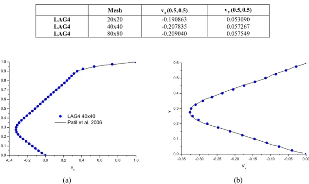
Using the numerical solution for the velocities vx and vy at (x, y) = (0.5, 0.5) presented in Table 4, it is possible to apply Equation (21) and compute the apparent order of the numerical solution. The estimated orders for the velocities vx and vy were, respectively, 3.82 and 3.89, which are in accordance with the fourth order of accuracy proposed in the formulation of the Lagrange schemes.

Comparing the velocity profiles obtained by the

LAG4 scheme with a 30x30 mesh with the results of Patil et al. (2006), who applied the lattice Boltzmann equation method using 256 lattice nodes in each coordinate direction, Figure 14, it is possible to observe a good agreement between the profiles obtained, especially considering the lower mesh refinement applied to the LAG4 schemes.

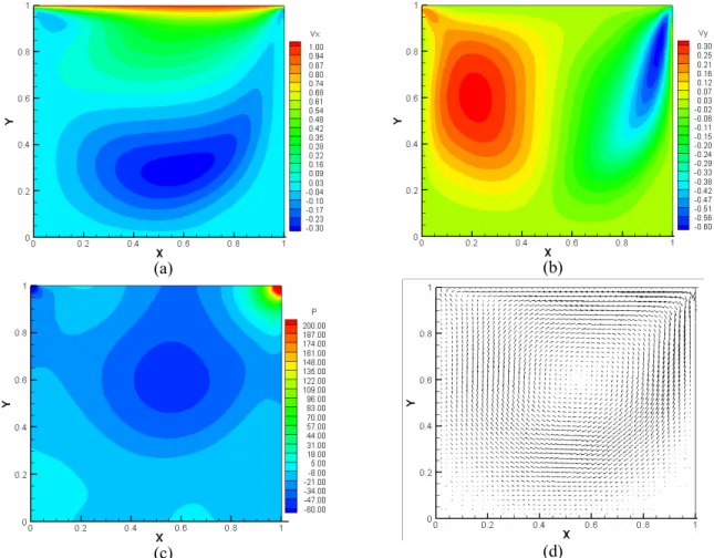
Figure 15 shows the velocity and pressure contour plots and the velocity vector for the lid-driven flow for Re=400, using the LAG4 scheme with a 50x50 mesh. Analyzing the contour plots for the velocity vx, Figure 15a, it is possible to observe two distinct regions of flow, the first near the cavity surface and the second near the bottom of the cavity. The first region is formed due to the proximity of the moving plate and the second region arises from the recirculation of fluid at the bottom of the cavity. For the velocity vy the presence of two distinct regions is also observed, the first on the right side of the plate with negative values of vy and the second on the left side of the plate with positive values of vy (Figure 15b). This signal change occurs due to the recirculation of fluid in the cavity, as can be seen in Figure 15d.

Table 4: Numerical solution for vx(0.5,0.5) and vy(0.5, 0.5) by applying the LAG4 scheme using refinements 20x20; 40x40 and 80x80 for Re=100.

Mesh v (0.5, 0.5)_x v (0.5, 0.5) y

LAG4 20x20 -0.190863 0.053090

LAG4 40x40 -0.207835 0.057267

LAG4 80x80 -0.209040 0.057549

-0.4 -0.2 0.0 0.2 0.4 0.6 0.8 1.0 0.0

0.1 0.2 0.3 0.4 0.5 0.6 0.7 0.8 0.9 1.0

y

v_x

LAG4 40x40 Patil et al. 2006

-0.35 -0.30 -0.25 -0.20 -0.15 -0.10 -0.05 0.00 0.0

0.1 0.2 0.3 0.4 0.5 0.6

y

V_x

(a) (b)

Brazilian Journal of Chemical Engineering

(a) (b)

(c) (d)

Figure 15: Contour plots obtained by applying the LAG4 scheme with a 50x50 mesh for Re=400: (a) Contour plot for velocity vx; (b) Contour plot for velocity vy; (c) Contour plot for pressure and (d) Velocity vector.

CONCLUSION

The application of higher-order interpolation schemes with multiblock partition was able to reduce considerably the computational effort employed in the simulation of all the problems tested. The application of the fourth-order Lagrange interpolation scheme was able to obtain solutions with the same degree of accuracy as other low-order procedures, requiring much less computational time by employing coarser grids.

The multiblock procedure was able to properly connect meshes with different degrees of refinement. The most important aspect of this procedure is the direct use of the interpolation formulas, ensuring that the global order of the approximation is maintained and allowing the application of any other interpolation scheme. The results obtained by application of the procedure proved its effectiveness where it was possible to refine only the regions of

interest, reducing significantly the simulation time without losing accuracy.

The joint use of high-order schemes and the multiblock partition technique allowed the development of a computer code with the higher accuracy of the high-order interpolation schemes and the flexibility of multiblock partitioning, reducing significantly the computational effort compared to traditional procedures.

REFERENCES

Barad, M., Colella, P., A fourth-order accurate local refinement method for Poisson’s equation. Journal of Computational Physics, 209, 1-18 (2005).

 

Brazilian Journal of Chemical Engineering Vol. 29, No. 01, pp. 183 - 201, January - March, 2012

Bird, R. B., Stewart, W. E. and Lightfoot, E. N., Transport Phenomena. 2nd Ed. John Wiley and Sons, USA (2002).

Botella, O. and Peyret, R., Benchmark spectral results on the lid-driven cavity flow. Computers and Fluids, 27, 421-433 (1998).

Bruneau, C. -H. and Jouron, C., An efficient scheme for solving steady incompressible Navier-Stokes Equations. Journal of Computational Physics, 89, 389-413 (1990).

Cebeci, T., Shao, J. P., Kafyere, F. and Laurendeau, E., Computational Fluid Dynamics for Engineers. 1st Ed. Springer, USA (2005).

Chen, W. L., Lien, F. S. and Laschziner, M. A., Local mesh refinement within a multi-block structured-grid scheme for general flows. Computer Method Applied Mechanics Engineering, 144, 327-369 (1997).

Deng, G. B., Piquet, J., Queutey, P. and Visonneau, M., Incompressible flow calculations with a consistent physical interpolation finite volume approach. Computers and Fluids, 23, 1029-1047 (1994).

Farrashkhalvat, M. and Miles, J. P., Basic structured grid generation. 1st Ed. Butterworth Heinemann, London (2003).

Ferziger, J. C. and Peric, M., Computational methods for fluid dynamics. 3rd Ed. Springer, New York, (2002).

Ghia, U., Ghia, K. N. and Shin, C. T., High-Re solutions for incompressible flows using the Navier-Stokes equations and a multigrid method. Journal of Computational Physics, 48, 387-411 (1982).

Hirsch, C., Numerical computation of internal and external flows. 2nd Ed. Elsevier, USA (2007). Kobayashi, M. H., On a class of Padé finite volume

method. Journal of Computational Physics, 156, 137-180 (1999).

Lacor, C., Smirnov, S. and Baelmans, M., A finite volume formulation of compact central schemes on arbitrary structured grids. Journal of Computational Physics, 198, 535-566 (2004). Leonard, B. P., Order of accuracy of QUICK and

related convection-diffusion schemes. Appl.

Math. Modeling, 19, 640-653 (1995).

Liu, J. and Shyy, W., Assessment of grid interface treatments for multi-block incompressible viscous flow computation. Computer and Fluids, 25, 719-740 (1996).

Muniz, A. R., Development of a high order finite volume method for simulation of viscoelastic fluid flow. D.Sc. Thesis, Federal University of Rio Grande do Sul-Brazil (2003).

Muniz, A. R., Secchi, A. R. and Cardozo, N. S. M., High-order finite volume method for solving viscoelastic fluid flows. Brazilian Journal of Chemical Engineering, 25, 1-14 (2008).

Patankar, S. V., Numerical heat transfer and fluid flow. 1st Ed. Hemisphere Publishing Corporation, USA (1980).

Patil, D. V., Lakshmisha, K. N. and Rogg, B., Lattice Boltzmann simulation of lid-driven flow in deep cavities. Computers and Fluids, 35, 1116-1125 (2006).

Pereira, J. M. C., Kobayashi, M. H. and Pereira, J. C. F., A fourth-order-accuracy finite volume compact method for the incompressible Navier-Stokes solutions. Journal of Computational Physics, 167, 217-243 (2001).

Piller, M. and Stalio, E., Finite volume compact scheme on staggered grids. Journal of Computational Physics, 197, 299-340 (2004). Secchi, A. R., DASSLC User’s Manual Version 3.2.

Universidade Federal do Rio Grande do Sul, DEQUI, Porto Alegre, RS, Brasil (2007).

Serón, F. S. and Sabadell, F. J., The multiblock method. A new strategy based on domain decomposition for the solution of wave propagation problems. International Journal for Numerical Methods in Engineering, 49, 1353-1376 (2000).

Versteeg, H. K. and Malalasekera, W., Introduction to computational fluid dynamics - The finite volume method. 2nd Ed. Person Prentice Hall, England (2007).

Brazilian Journal of Chemical Engineering APPENDIX

Fourth-order Lagrange interpolation formula for advective terms

APPROXIMATION FORMULA ERROR

( )

y

( )

xy

( )

xy

( )

xy

( )

xy

3 1 1 3

i i i i i

2 2 2 2

1 7 7 1

12 − 12 − 12 + 12 +

ϕ = − ϕ + ϕ + ϕ − ϕ 4 4

4 1 x 30 x ∂ ϕ − Δ ∂

( )

y

( )

xy

( )

xy

( ) ( )

xy xy

1 3 5 7

0

2 2 2 2

25 23 13 1

12 12 12 4

ϕ = ϕ − ϕ + ϕ − ϕ 4

4 4 1 x 5 x ∂ ϕ − Δ ∂

( ) ( )

y xy

( )

xy

( )

xy

( )

xy

1 3 5 7

1

2 2 2 2

1 13 5 1

4 12 12 12

ϕ = ϕ + ϕ − ϕ + ϕ 4 4

4 1 x 20 x ∂ ϕ Δ ∂

( )

y

( )

xy

( )

xy

( )

xy

( )

xy

7 5 3 1

N 1 N N N N

2 2 2 2

1 5 13 1

12 12 12 4

− − − − −

ϕ = ϕ − ϕ + ϕ + ϕ 4 4

4 1 x 20 x ∂ ϕ Δ ∂

( )

y

( )

xy

( )

xy

( )

xy

( )

xy

7 5 3 1

N N N N N

2 2 2 2

1 13 23 25

4 − 12 − 12 − 12 −

ϕ = − ϕ + ϕ − ϕ + ϕ 4

4 4 1 x 5 x ∂ ϕ − Δ ∂

Fourth-order Lagrange interpolation formula for diffusive terms

APPROXIMATION FORMULA ERROR

( )

( )

( )

( )

y

xy xy xy xy

3 1 1 3

i i i i

2 2 2 2

i

1 1 5 5 1

x x 12 − 4 − 4 + 12 +

⎛ ⎞

⎛_∂ϕ ⎞

⎜ ⎟

⎜ ⎟ = ϕ − ϕ + ϕ − ϕ

⎜ ∂ ⎟ Δ ⎜ ⎟

⎝ ⎠ ⎝ ⎠ 5 4 4 1 y 1920 y x

∂ ϕ

− Δ

∂ ∂

( )

( )

( )

( ) ( )

y

y xy xy xy xy

1 3 5 7

0

2 2 2 2

0

1 25 415 161 55 1

x x 6 72 72 72 8

⎛ ⎞

⎛_∂ϕ ⎞

⎜ ⎟

⎜ ⎟ = − ϕ + ϕ − ϕ + ϕ − ϕ

⎜ ∂ ⎟ Δ ⎜ ⎟

⎝ ⎠ ⎝ ⎠ 5 4 4 1 y 1920 y x

∂ ϕ

− Δ

∂ ∂

( ) ( )

( ) ( )

( )

y

y xy xy xy xy

1 3 5 7

1

2 2 2 2

1

1 5 1 23 4 1

x x 3 2 9 9 18

⎛ ⎞

⎛_∂ϕ ⎞

⎜ ⎟

⎜ ⎟ = − ϕ − ϕ + ϕ − ϕ + ϕ

⎜ ∂ ⎟ Δ ⎜ ⎟

⎝ ⎠ ⎝ ⎠

( )

( )

( )

( )

( )

xy xy xy

7 5 3

y _{N N N}

2 2 2

xy y

N 1 1

N N 1

2

1 4 23

18 9 9

1 1 5 x x 2 3 − − − − − −

⎛_{− ϕ + ϕ − ϕ +}⎞

⎜ ⎟

⎛_∂ϕ ⎞ _{⎜ ⎟}

⎜ ⎟ = _{⎜ ⎟}

⎜ ∂ ⎟ Δ _{ϕ + ϕ}

⎝ ⎠ _{⎜⎜ ⎟⎟} ⎝ ⎠ 5 4 4 5 4 5 5 2 4 3 2 1 y 1920 y x

1 x

24 x

1 y x

48 y x

∂ ϕ − Δ ∂ ∂ ∂ ϕ − Δ ∂ ∂ ϕ − Δ Δ

∂ ∂

( )

( )

( )

( )

( )

xy xy xy

7 5 3

y _{N N N}

2 2 2

xy y

N 1

N N

2

1 55 161

8 72 72

1 415 25 x x 72 6 − − − −

⎛ _{ϕ − ϕ + ϕ −}⎞

⎜ ⎟

⎛_∂ϕ ⎞ _{⎜ ⎟}

⎜ ⎟ = _{⎜ ⎟}

⎜ ∂ ⎟ Δ _{ϕ + ϕ}

⎝ ⎠ _{⎜ ⎟} ⎜ ⎟ ⎝ ⎠ 5 4 4 1 y 1920 y x

∂ ϕ

− Δ

 

Brazilian Journal of Chemical Engineering Vol. 29, No. 01, pp. 183 - 201, January - March, 2012

Fourth-order Lagrange interpolation formula for nonlinear terms

( ) ( ) ( )

( 0 0) ( 0 0)

( )

2

x x x 1 2 4

1 2 1 2

i i i _{x ,y x ,y}

x

O h

12 x x

⎛ ⎞⎛ ⎞

Δ _⎜⎛∂ϕ ⎞ _⎟⎜⎛∂ϕ ⎞ _⎟

ϕ ϕ = ϕ ϕ + _{⎜ ⎟ ⎜ ⎟} +

⎜⎝ ∂ ⎠ ⎟⎜⎝ ∂ ⎠ ⎟

⎝ ⎠⎝ ⎠

( ) ( ) ( )

( 0 0) ( 0 0)

( )

2

y y y 1 2 4

1 2 1 2

i i i _{x ,y x ,y}

y

O h

12 y y

⎛_{⎛ ⎞} ⎞⎛_{⎛ ⎞} ⎞

Δ _⎜ ∂ϕ _⎟⎜ ∂ϕ _⎟

ϕ ϕ = ϕ ϕ + _{⎜ ⎟ ⎜ ⎟} +

⎜_⎝ ∂ _⎠ ⎟⎜_⎝ ∂ _⎠ ⎟

⎝ ⎠⎝ ⎠

Approximation of the derivative with respect to x in the face of the control volume

APPROXIMATION FORMULA ERROR

( )

( )

( )

( )

xy xy xy

1

3 1 1 1 3 1

1

i , j i , j i , j

i , j

2 2 2 2 2 2

2 xy

1 1 i , j

2 2

1 1 1

x

x 4 4 4

1 4 + − − − + + + − + ∂ϕ ⎛ ⎞

Δ _{⎜ ⎟} = ϕ − ϕ + ϕ

∂ ⎝ ⎠ − ϕ 3 2 2 3 3 3 1 y x

6 y x

5 x 24 x ∂ ϕ Δ Δ ∂ ∂ ∂ ϕ + Δ ∂

( )

( )

( )

( )

( )

( )

xy xy xy

1

3 1

1 1 5 1

1 _{, j}

, j , j

, j _{2 2}

2 2 2 2

2

xy xy xy

3 1

1 1 _{, j} 5 1

, j , j

2 2

2 2 2 2

3 1

x

x 4 4

3 1 4 4 − − − + + + ∂ϕ ⎛ ⎞

Δ _{⎜ ⎟} = − ϕ + ϕ − ϕ

∂ ⎝ ⎠

− ϕ + ϕ − ϕ

3 2 2 3 3 3 1 y x

3 y x

5 x

24 x

∂ ϕ − Δ Δ

∂ ∂ ∂ ϕ + Δ ∂

( )

( )

( )

( )

( )

( )

xy xy xy

1

3 1

1 1 5 1

1 _{N , j N , j N , j}

N . j _{2 2}

2 2 2 2

2

xy xy xy

3 1

1 1 _{N , j} 5 1

N , j N , j

2 2

2 2 2 2

3 1

x

x 4 4

3 1 4 4 − − − − − − − − + − + − + ∂ϕ ⎛ ⎞

Δ _{⎜ ⎟} = ϕ − ϕ + ϕ

∂ ⎝ ⎠

+ ϕ − ϕ + ϕ

3 2 2 3 3 3 1 y x

3 y x

5 x

24 x

∂ ϕ − Δ Δ

∂ ∂ ∂ ϕ + Δ ∂

( )

( )

( )

( )

xy xy xy

1

3 1 1 1 3 3

1

i , i , i ,

i ,0

2 2 2 2 2 2

2 xy

1 3 i ,

2 2

3 3 1

x

x 4 4 4

1 4 + − + + − ∂ϕ ⎛ ⎞

Δ _{⎜ ⎟} = ϕ − ϕ − ϕ

∂ ⎝ ⎠ + ϕ 3 2 2 3 3 3 1 y x

6 y x

7 x 24 x ∂ ϕ Δ Δ ∂ ∂ ∂ ϕ + Δ ∂

( )

( )

( )

( )

xy xy xy

1

3 3 1 3 3 1

1

i ,N i ,N i ,N

i ,N

2 2 2 2 2 2

2 xy

1 1

i ,N

2 2

1 1 3

x

x 4 4 4

3 4 + − − − + − + − − ∂ϕ ⎛ ⎞

Δ _{⎜ ⎟} = − ϕ + ϕ + ϕ

∂ ⎝ ⎠ − ϕ 3 2 2 3 3 3 1 y x

6 y x

7 x 24 x ∂ ϕ Δ Δ ∂ ∂ ∂ ϕ + Δ ∂

( )

( )

( )

( ) ( )

( )

xy xy xy

1

3 1

1 1 5 1

1 _,

, ,

,0 _{2 2}

2 2 2 2

2

xy xy xy

3 3

1 3 _, 5 3

, ,

2 2

2 2 2 2

9 3

x 3

x 4 4

3 1

4 4

∂ϕ ⎛ ⎞

Δ _{⎜ ⎟} = − ϕ + ϕ − ϕ

∂ ⎝ ⎠

+ ϕ − ϕ + ϕ

3 2 2 3 3 3 1 y x

3 y x

7 x

24 x

∂ ϕ − Δ Δ

∂ ∂ ∂ ϕ − Δ

Brazilian Journal of Chemical Engineering

Continuation

Approximation of the derivative with respect to x in the face of the control volume

APPROXIMATION FORMULA ERROR

( )

( )

( )

( )

( )

( )

xy xy xy

1

3 3

1 3 5 3

1 _,N

,N ,N

,N _{2 2}

2 2 2 2

2

xy xy xy

3 1

1 1 _,N 5 1

,N ,N

2 2

2 2 2 2

3 1

x

x 4 4

9 3 3 4 4 − − − − − − ∂ϕ ⎛ ⎞

Δ _{⎜ ⎟} = ϕ − ϕ + ϕ

∂ ⎝ ⎠

− ϕ + ϕ − ϕ

3 2 2 3 3 3 1 y x

3 y x

7 x

24 x

∂ ϕ − Δ Δ

∂ ∂ ∂ ϕ − Δ ∂

( )

( )

( )

( )

( )

( )

xy xy xy

1

3 1

1 1 5 1

1 _{N ,}

N , N ,

N ,0 _{2 2}

2 2 2 2

2

xy xy xy

3 3

1 3 _{N ,} 5 3

N , N ,

2 2

2 2 2 2

9 3

x 3

x 4 4

3 1 4 4 − − − − − − − ∂ϕ ⎛ ⎞

Δ _{⎜ ⎟} = ϕ − ϕ + ϕ

∂ ⎝ ⎠

− ϕ + ϕ − ϕ

3 2 2 3 3 3 1 y x

3 y x

7 x

24 x

∂ ϕ − Δ Δ

∂ ∂ ∂ ϕ − Δ ∂

( )

( )

( )

( )

( )

( )

xy xy 1 3 3 1 3

1 _{N ,N N ,N}

N ,N _{2 2}

2 2

2

xy xy xy xy

3 1

5 3 1 1 _{N ,N} 5 1

N ,N N ,N N ,N

2 2

2 2 2 2 2 2

3 x

x 4

1 9 3

3

4 4 4

− − − − − − − − − − − − − ∂ϕ ⎛ ⎞

Δ _{⎜ ⎟} = − ϕ + ϕ

∂ ⎝ ⎠

− ϕ + ϕ − ϕ + ϕ

3 2 2 3 3 3 1 y x

3 y x

7 x

24 x

∂ ϕ − Δ Δ

∂ ∂ ∂ ϕ − Δ

∂

Approximation of the derivative with respect to y in the face of the control volume

APPROXIMATION FORMULA ERROR

( )

( )

( )

( )

xy xy xy

1

1 3 1 1 1 3

1 _{i , j i , j i , j}

i, j

2 2 2 2 2 2

2 xy

1 1 i , j

2 2

1 1 1

y

y 4 4 4

1 4

− + − − + +

+

+ −

⎛∂ϕ ⎞

Δ _{⎜ ⎟} = ϕ − ϕ + ϕ

∂ ⎝ ⎠ − ϕ 3 2 2 3 3 3 1 x y

6 x y

5 y 24 y ∂ ϕ Δ Δ ∂ ∂ ∂ ϕ + Δ ∂

( )

( )

( )

( )

xy xy xy

1

1 3 1 1 3 3

1 _{, j , j , j}

0, j

2 2 2 2 2 2

2 xy

3 1 , j 2 2

3 3 1

y

y 4 4 4

1 4

+ − +

+

−

⎛∂ϕ ⎞

Δ _{⎜ ⎟} = ϕ − ϕ − ϕ

∂ ⎝ ⎠ + ϕ 3 2 2 3 3 3 1 x y

3 x y

5 y

24 y

∂ ϕ − Δ Δ

∂ ∂ ∂ ϕ + Δ ∂

( )

( )

( )

( )

xy xy 1

3 3 3 1

1 _{N , j N , j}

N, j

2 2 2 2

2

xy xy

1 3 1 1

N , j N , j

2 2 2 2

1 1

y

y 4 4

3 3

4 4

− + − −

+

− + − −

⎛∂ϕ ⎞

Δ _{⎜ ⎟} = − ϕ + ϕ

∂ ⎝ ⎠

+ ϕ − ϕ

3 2 2 3 3 3 1 x y

3 x y

5 y

24 y

∂ ϕ − Δ Δ

∂ ∂ ∂ ϕ + Δ ∂

( )

( )

( )

( )

( )

( )

xy xy xy

1

1 3

1 1 1 5

1 _{i ,} i , _{i ,}

i, _{2 2}

2 2 2 2

2

xy xy xy

1 3

1 1 _{i ,} 1 5

i , i ,

2 2

2 2 2 2

3 1

y

y 4 4

3 1 4 4 − − − + + +

⎛∂ϕ ⎞

Δ _{⎜ ⎟} = − ϕ + ϕ − ϕ

∂ ⎝ ⎠

− ϕ + ϕ − ϕ

3 2 2 3 3 3 1 x y

6 x y

 

Brazilian Journal of Chemical Engineering Vol. 29, No. 01, pp. 183 - 201, January - March, 2012

Continuation

Approximation of the derivative with respect to y in the face of the control volume

APPROXIMATION FORMULA ERROR

( )

( )

( )

( )

( )

( )

xy xy xy

1

1 3

1 1 1 5

1 i ,N i ,N i ,N

i,N _{2 2}

2 2 2 2

2

xy xy xy

1 3

1 1 _{i ,N} 1 5

i ,N i ,N

2 2

2 2 2 2

3 1

y

y 4 4

3 1 4 4 − − − − − − − + − + − + −

⎛∂ϕ ⎞

Δ _{⎜ ⎟} = ϕ − ϕ + ϕ

∂ ⎝ ⎠

+ ϕ − ϕ + ϕ

3 2 2 3 3 3 1 x y

6 x y

7 y 24 y ∂ ϕ Δ Δ ∂ ∂ ∂ ϕ − Δ ∂

( )

( )

( )

( ) ( )

( )

xy xy xy

1

1 3

1 1 1 5

1 _, , _,

0, _{2 2}

2 2 2 2

2

xy xy xy

3 3

3 1 _, 3 5

, ,

2 2

2 2 2 2

9 3

y 3

y 4 4

3 1

4 4

⎛∂ϕ ⎞

Δ _{⎜ ⎟} = − ϕ + ϕ − ϕ

∂ ⎝ ⎠

+ ϕ − ϕ + ϕ

3 2 2 3 3 3 1 x y

3 x y

7 y

24 y

∂ ϕ − Δ Δ

∂ ∂ ∂ ϕ − Δ ∂

( )

( )

( )

( )

( )

( )

xy xy xy

1

1 3

1 1 1 5

1 ,N ,N ,N

0,N _{2 2}

2 2 2 2

2

xy xy xy

3 3

3 1 _,N 3 5

,N ,N

2 2

2 2 2 2

9 3

y 3

y 4 4

3 1 4 4 − − − − − − −

⎛∂ϕ ⎞

Δ _{⎜ ⎟} = ϕ − ϕ + ϕ

∂ ⎝ ⎠

− ϕ + ϕ − ϕ

3 2 2 3 3 3 1 x y

3 x y

7 y

24 y

∂ ϕ − Δ Δ

∂ ∂ ∂ ϕ − Δ ∂

( )

( )

( )

( )

( )

( )

xy xy xy

1

3 3

3 1 3 5

1 N , N , N ,

N, _{2 2}

2 2 2 2

2

xy xy xy

1 3

1 1 _{N ,} 1 5

N , N ,

2 2

2 2 2 2

3 1

y

y 4 4

9 3 3 4 4 − − − − − −

⎛∂ϕ ⎞

Δ _{⎜ ⎟} = ϕ − ϕ + ϕ

∂ ⎝ ⎠

− ϕ + ϕ − ϕ

3 2 2 3 3 3 1 x y

3 x y

7 y

24 y

∂ ϕ − Δ Δ

∂ ∂ ∂ ϕ − Δ ∂

( )

( )

( )

( )

( )

( )

xy xy xy

1

3 3

3 1 3 5

1 N ,N N ,N N ,N

N,N _{2 2}

2 2 2 2

2

xy xy xy

1 3

1 1 _{N ,N} 1 5

N ,N N ,N

2 2

2 2 2 2

3 1

y

y 4 4

9 3 3 4 4 − − − − − − − − − − − − −

⎛∂ϕ ⎞

Δ _{⎜ ⎟} = − ϕ + ϕ − ϕ

∂ ⎝ ⎠

+ ϕ − ϕ + ϕ

3 2 2 3 3 3 1 x y

3 x y

7 y

24 y

∂ ϕ − Δ Δ

∂ ∂ ∂ ϕ − Δ

∂

Deconvolution formula for the fourth-order Lagrange interpolation

APPROXIMATION FORMULA ERROR

( )

( )

x

( )

x

( )

x

( )

x

3 1 1 3

i

i i i i

2 2 2 2

1 7 7 1

12 − 12 − 12 + 12 +

ϕ = − ϕ + ϕ + ϕ − ϕ 4 4

4 1 x 30 x ∂ ϕ − Δ ∂

( )

( )

x

( )

x

( ) ( )

x x

1 3 5 7

0

2 2 2 2

25 23 13 1

12 12 12 4

ϕ = ϕ − ϕ + ϕ − ϕ 4

4 4 1 x 5 x ∂ ϕ − Δ ∂

( )

( )

x

( )

x

( )

x

( )

x

1 3 5 7

1

2 2 2 2

1 13 5 1

4 12 12 12

ϕ = ϕ + ϕ − ϕ + ϕ 4

4 4 1 x 60 x ∂ ϕ − Δ ∂

( )

( )

x

( )

x

( )

x

( )

x

N 1 7 5 3 1

N N N N

2 2 2 2

1 5 13 1

12 12 12 4

− _{− − − −}

ϕ = ϕ − ϕ + ϕ + ϕ 4 4

4 1 x 60 x ∂ ϕ − Δ ∂

( )

( )

x

( )

x

( )

x

( )

x

7 5 3 1

N

N N N N

2 2 2 2

1 13 23 25

4 − 12 − 12 − 12 −

ϕ = − ϕ + ϕ − ϕ + ϕ 4