D. Strauss and
J. L. F. Azevedo
Instituto de Aeronáutica e Espaço Centro Técnico Aeroespacial CTA/IAE/ASE-N 12228-904 São José dos Campos, SP. Brazil [email protected]
On the Development of an
Agglomeration Multigrid Solver for
Turbulent Flows
The paper describes the implementation details and validation results for an agglomeration multigrid procedure developed in the context of hybrid, unstructured grid solutions of aerodynamic flows. The governing equations are discretized using an unstructured grid finite volume method, which is capable of handling hybrid unstructured grids. A centered scheme as well as a second order version of Liou’s AUSM+ upwind scheme are used for the spatial discretization. The time march uses an explicit 5-stage Runge-Kutta time-stepping scheme. Convergence acceleration to steady state is achieved through the implementation of an agglomeration multigrid procedure, which retains all the flexibility previously available in the unstructured grid code. The calculation capability created is validated considering 2-D laminar and turbulent viscous flows over a flat plate. Studies of the various parameters affecting the multigrid acceleration performance are undertaken with the objective of determining optimal numerical parameter combinations.
Keywords: Agglomeration multigrid, convergence acceleration, unstructured grids, finite
volume methods
Introduction
Many different convergence acceleration methods have been developed and discussed in the literature in the past years. These methods involve various aspects of the numerical solution of partial differential equations and demand implementation efforts which can be very simple or very complex. The implementation of a variable time step option and optimized time stepping schemes yields a solution to the convergence acceleration problem, which demands a relatively small effort. On the other hand, time-implicit schemes and multigrid procedures also solve the problem but are much more demanding. A combination of these convergence acceleration methods usually gives the best overall result.1
Unstructured meshes present additional difficulties to the implementation of some of the convergence acceleration methods when compared to structured grids. For instance, implicit time-stepping schemes are handicapped by the need of using indirect addressing in order to express the mesh connectivity, resulting in a more difficult implementation and a reduced gain in efficiency. Furthermore, the structure of the linear systems, which appear in the unstructured grid case, involves matrices which are sparse but not banded. Hence, the linear system solvers are inherently more expensive than their structured grid counterparts. Multigrid procedures are also more difficult to implement in unstructured meshes, mainly due to the burden of obtaining the coarse meshes. However, the gains of a multigrid procedure for unstructured meshes are very significant and, therefore, the additional work is worthwhile.
The main concern in the implementation of a multigrid procedure for unstructured meshes is the generation and treatment of the coarse meshes. There are basically three different ways of handling this problem. In the first approach, the fine meshes are obtained by refinement of the coarse meshes, resulting in nested meshes (Mavriplis, 1988). This approach often results in problems in obtaining an adequate mesh refinement in the regions of interest. An exception to this statement would be the case in which the multigrid algorithm is necessarily coupled to a solution adaptive grid refinement procedure. In this case, however, one would start from the coarsest mesh and would let the adaptive refinement
Paper accepted August, 2003. Technical Editor: Aristeu da Silveira Neto.
procedure produce the finer meshes for the application of the multigrid method. Nevertheless, this is a very particular case and it requires a very well tuned adaptive refinement procedure, especially for viscous turbulent flows. Another approach considers coarse meshes that are generated independently from the fine meshes, such that the meshes are unrelated or non-nested (Mavriplis, 1988, 1990, Mavriplis and Jameson, 1990). This approach has the inconvenience of requiring the calculation of the intersections between the coarse and fine mesh volumes, which can be very difficult in the general case. Moreover, the generation of the coarse meshes itself also requires a substantial amount of work. Finally, the third approach is the agglomeration technique (Mavriplis and Venkatakrishnan, 1994, Venkatakrishnan and Mavriplis 1995). In this case, the coarse meshes are generated by agglomerating the neighboring volumes of the fine meshes. Hence, this approach does not have the disadvantages of the others and it was the one chosen by the authors in this work.
This work, then, describes the implementation details and validation results for an agglomeration multigrid procedure. The procedure is developed in the context of a 2-D Reynolds-averaged Navier-Stokes solver, capable of handling hybrid, unstructured grids. The governing equations are discretized both with a centered and an upwind finite volume method. Time march uses an explicit 5-stage Runge-Kutta time-stepping scheme. The upwind scheme implemented is a second order version of the Liou AUSM+ scheme (Liou, 1996). Moreover, the turbulent effects are accounted for by the Baldwin and Barth (1990) and Spalart and Allmaras (1994) turbulence closure models. Laminar and turbulent viscous flow simulations over a flat plate are used to validate the present implementation. Studies of the various parameters affecting the multigrid acceleration performance are undertaken with the objective of determining optimal numerical parameter combinations.
Nomenclature
English Symbols
a = speed of sound
ci’s = turbulence model constants
d = distance to the wall E,F = flux vectors
e = total energy
∞
M = freestream Mach number
p = static pressure
P, S~ = production terms
Q = vector of conserved variables
qx, qy = heat flux vector components
Rel = Reynolds number based on the total plate length
T
R~ = turbulence Reynolds number
S = area t = time
u = Cartesian component of the velocity vector in the x direction v = Cartesian component of the velocity vector in the y direction V = volume
V = velocity vector
y+ = nondimensional wall coordinate Greek Symbols
t
∆ = time step
γ = ratio of specific heats
κ = von Kármán constant
µ = laminar dynamic viscosity coefficient
t
µ = turbulent dynamic viscosity coefficient
ν = laminar kinematic viscosity coefficient
t
ν = turbulent kinematic viscosity coefficient
ρ = density
ρw = wall density
σi’s = turbulence model constants
yy xy xx τ τ
τ , , = components of the viscous stress tensor
τw = wall viscous stress
ω = magnitude of the vorticity vector
∇ = Gradient operator
2
∇ = Laplacian operator
Multigrid Implementation
Multigrid Procedure
Multigrid methods have been developed for the solution of general partial differential equations on a discretized domain (Brandt, 1977). Therefore, in this section, a general discussion of the implementation of a Full Approximation Storage (FAS) multigrid algorithm will be presented. For such discussion, consider a problem written in the operator form as
( )
u =0L . (1)
The discretized problem that has to be solved is
( )
h h h u fL = , (2)
where the discretization in which a solution is wanted is represented by h. With the use of the multigrid procedure, the discretized problem is solved on a coarser mesh H. As the H mesh has fewer points than the h mesh, the solution of the problem in the H mesh requires a lower computational cost than in the h mesh. Hence, the problem in the H mesh can be written as
( )
H HH u f
L = , (3)
with
( )
hH h h H h H
H L I u I r
f = − , (4)
( )
h h hh L u f
r = − , (5)
and fh = 0 in the finest mesh. The
H h
I operator is the restriction operator, which transfers the properties from the fine to the coarse mesh. The solution in the h mesh is updated from the solution of Eq.
(3) using the prolongation operator IHh , which transfers the
properties from the coarse to the fine mesh. Hence, solution update in the h mesh can be written as
(
H hH h)
h H h new
h u I u I u
u = + − . (6)
It should be noted that the multigrid procedure can be applied successively using coarser and coarser meshes. Therefore, Eq. (3) can also be solved through the multigrid procedure, but using an even coarser mesh 2H.
For correction operators written in delta form, the problem to be solved is
( )
(
n n) ( )
nu R u u N u
L = +1− + . (7)
In the last equation, the N operator is associated with the properties update, while the R operator is associated with the discretization of the problem equations. In this case, the correction operator can represent a relaxation method or a time marching scheme. If the operator in Eq. (7) is rewritten in the discretized form of Eq. (3), the problem that should be solved in the coarse mesh is obtained as
( )
(
) ( )
nH n H H n H n H H H
H u N u u R u f
L = +1− + = . (8)
Equations (4) and (5), then, become
(
) ( )
nh n h h n h n h h n
h N u u R u f
r = +1− + − , (9)
(
hH hn1 hH hn) ( )
H hHhn hH[
h(
hn1 hn) ( )
h hn hn]
.H n
H N I u I u R I u I N u u R u f
f = + − + − + − + −
(10)
If one defines
( )
[
( )
n]
h n h h H h n h H h H n
H R I u I R u f
F = − − , (11)
Equation (10) transforms to
(
)
[
(
n)
]
h n h h H h n h H h n h H h H n H n
H F N I u I u I N u u
f = + +1− − +1− . (12)
In order to obtain the solution of Eq. (8), it is necessary to calculate all the terms in Eq. (12). However, the two last terms of Eq. (12) are not known because they involve the solution on the fine mesh on the n + 1-th time step. Hence, these terms are calculated with a time delay, that is, in the n-th time step. Using the definition of the problem, Eq. (8), and this concept of time delay, one can obtain the following results
(
− −1)
= −1−( )
n−1h h n h n h n h
h u u f R u
N , (13)
(
− −1)
= −1−(
n−1)
h H h H n H n h H h n h H h
H I u I u f R I u
The substitution of Eqs. (13) and (14) in Eq. (12) yields
(
1)
[
1( )
1]
1 − − −
− − − −
+
= n
h h n h H h n h H h H n H n H n
H F f R I u I f R u
f , (15)
or, if one uses Eq. (11),
1
1 −
− −
+
= n
H n H n H n
H F f F
f . (16)
Equation (16) can be used to obtain the value of
f
Hn−1, resulting1 2 2
1 − − −
− + − −
+
= n
H n H n H n H n H n
H F F f F F
f . (17)
In this equation, the
F
Hn−1 terms cancel each other, so there is no contribution of the n - 1-th instant of time. After successive application of Eq. (17), the only contribution left will be that of the initial instant of time, which can be neglected. Therefore, the final problem that has to be solved is(
) ( )
nH n H H n H n H
H u u R u F
N +1− + = , (18)
with
( )
[
( )
n]
h n h h H h n h H h H n
H R I u I R u f
F = − − . (19)
Agglomeration Technique
The previous section discussed the multigrid implementation in a general way. There was no attempt to treat the practical issues associated with such implementation. In this section, the actual implementation of the agglomeration procedure for generating the coarse meshes will be addressed.
The coarse meshes for the multigrid procedure are generated by agglomerating or grouping fine mesh volumes to form one coarse mesh volume. A “seed” volume is chosen in the fine mesh and, then, all the volumes that have a node or an edge in common with this “seed” volume are grouped in order to form the coarse mesh volume. Another “seed” volume is selected and the agglomeration procedure continues grouping all the fine mesh volumes. It should be noted that during the agglomeration procedure only the volumes that have not already been agglomerated may be grouped to form a coarse mesh volume. This is a necessary condition in order to guarantee that there is no volume overlapping in the coarse mesh.
Better coarse mesh quality can be obtained if the selection of the “seed” volumes is not random. Therefore, a list containing all the fine mesh volumes is generated prior to the agglomeration procedure. In this work, the list is formed such that the first volumes are the volumes next to a boundary and, only after them, come the interior volumes. This approach is very simple, easy to implement and adds a very low additional computational cost. Although it does not necessarily provide the best agglomeration of the interior volumes, it results in good quality coarse mesh volumes close to the boundaries.
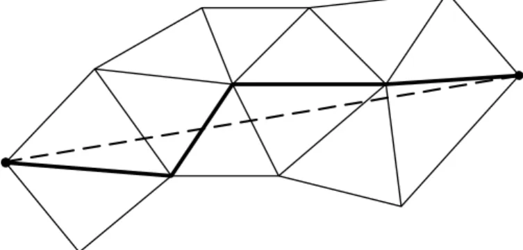
As the spatial discretization scheme used in this work can be interpreted as a line integral, a simplification can be made in the coarse meshes. This simplification consists in eliminating the nodes that belong to only two volumes. The justification for this procedure comes from the fact that the flux passing between the two volumes is the same whether the boundary separating the two volumes is discretized by one or many edges, provided that the discretization scheme is linear. Therefore, a significant amount of storage space can be saved by doing this mesh simplification. Figure 1 presents an
example of such node elimination, in which the darker lines represent the original boundary separating two coarse volumes and the dashed line represents the boundary edge after the node elimination.
Figure 1. Mesh simplification by the node elimination procedure.
Although the mesh simplification previously described can reduce the total storage space required by the code, it brings a complication related to the connectivity of the nodes in the mesh. As some nodes in the mesh are not used, it is necessary to ensure that the remaining nodes are properly counterclockwise oriented in order to have the normal vectors of each edge correctly pointing outwards. This is accomplished using the node orientation in the fine mesh volumes to orient the nodes in the coarse mesh volumes.
The agglomeration procedure can be summarized, then, in three steps. The first step consists in defining the list of fine mesh volumes. In the second step, the fine mesh volumes are agglomerated to form the coarse mesh volumes, following the list generated in the first step. During this step, the mesh simplification described is adopted and only the nodes that belong to three or more coarse mesh volumes are stored. The third and final step is the verification of the node orientation in each volume of the coarse mesh and the correction of the orientation where it is needed.
The actual implementation of this agglomeration procedure was designed to require the minimum amount of storage possible. Therefore, the only extra information that has to be stored in each mesh, besides the usual information associated with the solution procedure, is the number of the coarse mesh volume that contains each of the fine mesh volumes.
Restriction and Prolongation Operators
In the description of the multigrid procedure, the restriction and prolongation operators were introduced. Their actual mathematical definition was not presented in the last sections, but it will be discussed in this section. The restriction operator for the conserved properties, as well as for the residuals, will be presented together with two different prolongation operators for the conserved properties.
volume schemes. Consequently, as the residuals of the fine mesh are summed, the interior edge contributions will cancel each other, leaving only the contribution of the edges that form the coarse mesh volume.
The prolongation operator, in opposition to the restriction operator, transfers a variable from a coarse mesh to a fine mesh. As discussed in the Multigrid Procedure section, only the conserved property corrections have to be prolonged. Hence, only one prolongation operator has to be defined. In this work, two such different operators were used. The first operator uses direct injection of the coarse mesh values into the fine mesh. With this operator, the correction of a fine mesh volume is equal to the correction of the coarse mesh volume that contains that volume. Although this operator is very simple and easy to implement, it is not able to transfer exactly even a linear distribution. The second prolongation operator uses an averaging process to obtain the corrections in the fine grids. The averaging consists in, for each edge of the fine mesh, arithmetically averaging the corrections of the coarse mesh volumes corresponding to the two volumes that contain the edge. For each volume, then, these averaged corrections are added and the result is divided by the number of edges of the volume. This operator is also very easy to implement, and it has the advantage of being able to transfer a linear distribution with less error than the first prolongation operator. As it will be shown latter in the paper, the second option results in better convergence rates for viscous flows.
Theoretical Formulation
The agglomeration multigrid procedure previously described is applied to the solution of the Reynolds-averaged Navier-Stokes equations, which can be written in integral form as
(
−)
=0+ ∂∂ V
∫
S∫
dx dy dV
t Q E F , (20)
where
( )
( )
⎪⎪⎭ ⎪ ⎪ ⎬ ⎫ ⎪ ⎪ ⎩ ⎪ ⎪ ⎨ ⎧ + − − + − − = ⎪ ⎪ ⎭ ⎪ ⎪ ⎬ ⎫ ⎪ ⎪ ⎩ ⎪ ⎪ ⎨ ⎧ + − − + − − + = ⎪ ⎪ ⎭ ⎪⎪ ⎬ ⎫ ⎪ ⎪ ⎩ ⎪⎪ ⎨ ⎧ = y yy xy yy xy x xy xx xy xx q v u v p e v uv v q v u u p e uv p u u e v u τ τ τ ρ τ ρ ρ τ τ τ ρ τ ρ ρ ρ ρρ 2 2 ,, E F
Q
. (21)
The correct account for all the relevant flow phenomena in the present case involves the implementation of an appropriate turbulence closure model. The turbulence closure models implemented in this work were the Baldwin and Barth (1990) and the Spalart and Allmaras (1994) one-equation models. These models attempt to avoid the need to compute algebraic length scales, without having to resort to more complex two-equation, or κ - ε type models. The models were implemented in the present code precisely as described in Baldwin and Barth (1990) original work and in Spalart and Allmaras (1994) original work, for the case with no laminar regions. The extension of both models for compressible flows was obtained simply by multiplying the kinematic turbulent viscosity coefficient by the local density, as indicated in the respective original papers. Moreover, the turbulence model equation is solved separately from the other governing equations in a loosely coupled fashion (Baldwin and Barth, 1990).
The Baldwin and Barth (1990) model partial differential equation is
( )
(
)
( )
( )
( )
⎥ ⎥ ⎦ ⎤ ⎢ ⎢ ⎣ ⎡ ∇ ⋅ ∇ − ∇ ⎟⎟⎠ ⎞ ⎜⎜⎝ ⎛ + + −= T t T t T
T c f c R P R R
Dt R
D ~ ~ 2 ~ 1 ~
2 1
2 σ ν σ ν ν
ν ν ν ν ε ε ε ε . (22)
In the previous equation,
( )
( )
+ ⋅∇( )
∂∂ = V t Dt D is the
material derivative, which contains the time derivative and convective terms. The first term on the right hand side of this equation is the production term and the terms between the square brackets are the diffusion terms. This equation is solved for the product of variables
( )
RT~
ν and the eddy viscosity is calculated as
( )
Tt c DD R
~
2
1 ν
ρ
µ = µ , (23)
where the damping functions D1 and D2 are designed to allow the model to be used in the near-wall region.
The Spalart and Allmaras (1994) model partial differential equation is
(
)
(
)
( )
[
]
. ~ ~ ~ ~ . 1 ~ ~ ~ 2 1 2 2 1 ⎟ ⎠ ⎞ ⎜ ⎝ ⎛ − ∇ + ∇ + ∇ + = d f c c S c Dt D w w bb ν ν ν ν ν
σ ν
ν (24)
The first term on the right hand side of the equation is the production term. Moreover, the last term of this equation is the destruction term and the other terms are the diffusion terms. This equation is solved for the variable
ν
~
and the eddy viscosity is calculated as1
~
v t ρνf
µ = , (25)
where the function fv1 is a damping function used to properly treat
the buffer layer and the viscous sublayer.
Numerical Formulation
Using a cell centered based finite volume scheme, the discrete vector of conserved variables is defined as an average over the cell of the continuous properties. Hence, for the i-th volume the discrete property vector is
∫
= i V i i dV V QQ 1 . (26)
The definition of the discrete vector Qi can be used to rewrite
Eq. (20), resulting
( ) (
+ −)
=0∂∂
∫
i
S i
i dy dx
V
t Q E F . (27)
(
)
∑
[
]
∫
− = n= ∆ − ∆k
ik ik ik ik S
x y
dx dy
i 1
F E
F
E . (28)
When the central difference scheme is used as the spatial discretization scheme in Eq. (28), artificial dissipation terms must be added in order to control nonlinear instabilities (Jameson and Mavriplis, 1986). In the present case, the artificial dissipation operator is formed as a blend of undivided Laplacian and biharmonic operators (Mavriplis, 1988, 1990). The expressions for this operator can be found, for instance, in Azevedo and Korzenowski (1998). Moreover, the scaling terms of the artificial dissipation model were implemented following two approaches: Jameson and Mavriplis’ (1986) work and Mavriplis’ (1990) work.
The Liou scheme (Liou, 1996) implementation follows the work in Azevedo and Korzenowski (1998) and Strauss and Azevedo (2001) for both the first and second order versions of the scheme. The second order version of the scheme is obtained by following exactly the same formulation of the first order version, except that the left and right states are obtained by a MUSCL extrapolation of primitive variables (van Leer, 1979). The interested reader is referred to the original work of van Leer (1979) for details on the definition of the MUSCL scheme. In this work, cell averaged property gradients are computed and used to calculate the extrapolated properties (Barth and Jespersen, 1989). Gradients are computed here in the standard finite volume fashion, in which the derivatives are calculated in each volume considering that the discrete derivative in a given volume is the average on the volume of the derivative and, then, using Green’s theorem to transform the computation of the derivative on the computation of a line integral. The line integral calculation is performed in two quite different forms in the present work. In one approach, the control volumes used for the cell averaged gradient calculations are the volumes themselves. This is the simplest approach possible, but it is usually criticized in the literature(Barth and Jespersen, 1989), because it cannot recover the correct gradient of a linear function. The second approach implemented here consists of defining the control volume for the gradient calculation as the polygon formed by connecting the centroids of all cells which have an edge or a vertex in common with the volume for which the gradients are being computed, as suggested by Barth and Jespersen (1989). These two different forms of defining the control volumes are illustrated in Fig. 2 for the i-th volume. The simplified control volume is indicated by the darker lines in this figure, while the extended control volume is indicated by the dashed lines.
i
Figure 2. Control volumes for the gradient computation.
With the property extrapolation, the state variables are represented as piecewise linear within each cell, instead of piecewise constant. Hence, in order to avoid oscillations in the
solution due to the property extrapolation, it is necessary to use a limiter. The minmod limiter was implemented, following the work in Barth and Jespersen (1989). In order to obtain a better convergence rate, the limiter value is “frozen” after a certain number of iterations, as described in Venkatakrishnan (1995). This procedure avoids the convergence stall commonly observed when second-order schemes based on linear reconstruction of variables are used (Venkatakrishnan, 1995).
Results and Discussion
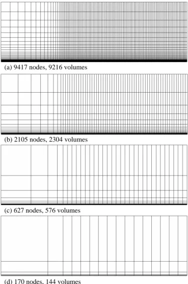
The multigrid procedure described in the previous sections is applied in the solution of laminar viscous flow over a flat plate configuration at zero angle of attack. This quite simple problem was chosen in order to provide a model problem which could be used to assess the convergence acceleration performance of the multigrid procedure. Different parameters of the multigrid procedure were tested in an attempt to determine the settings that would result in the best convergence acceleration.
(a) 9417 nodes, 9216 volumes
(b) 2105 nodes, 2304 volumes
(c) 627 nodes, 576 volumes
(d) 170 nodes, 144 volumes
Figure 3. Fine (a) and coarse agglomerated meshes (b, c, d) used for the flat plate calculations.
using an unstructured mesh generated from a structured mesh was made because a structured mesh is very easy to generate in this case and quadrilateral cells are more adequate to the treatment of viscous flows adjacent to solid walls. On the other hand, since the complete procedure treats all meshes as fully unstructured, the capability could be directly applied to any other grid configuration.
In the simulation, the flow characteristics used were M∞ = 0.3 and Rel = 1.0 × 10
5
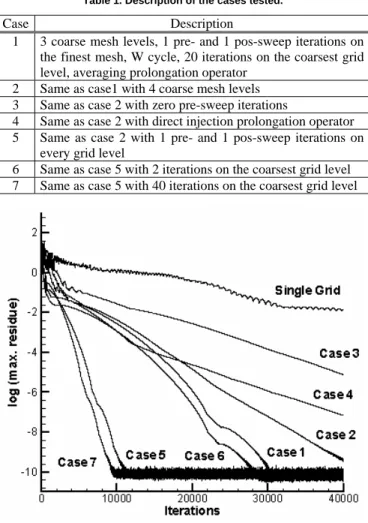
based on the total plate length. The centered scheme with Jameson and Mavriplis’ (1986) artificial dissipation model was used. Many different numerical parameters were tested in order to assess the optimal settings that would result in the best convergence ratios. A summary of the cases tested is presented in Table 1 and the convergence histories corresponding to these cases are presented in Fig. 4. In this figure, the convergence history for the case of no multigrid procedure is also shown and it is labeled as “single grid case”.
Table 1. Description of the cases tested.
Case Description 1 3 coarse mesh levels, 1 pre- and 1 pos-sweep iterations on
the finest mesh, W cycle, 20 iterations on the coarsest grid level, averaging prolongation operator
2 Same as case1 with 4 coarse mesh levels 3 Same as case 2 with zero pre-sweep iterations
4 Same as case 2 with direct injection prolongation operator 5 Same as case 2 with 1 pre- and 1 pos-sweep iterations on
every grid level
6 Same as case 5 with 2 iterations on the coarsest grid level 7 Same as case 5 with 40 iterations on the coarsest grid level
Figure 4. Convergence histories for the cases described in Table 1.
The convergence histories presented in Fig. 4 cannot be used to directly compare the performance of the multigrid procedure, as the computational cost per iteration is different in each case tested. Therefore, a comparison in terms of computational time is presented in Table 2. From this table, it can be seen that it is worthwhile to spend more in the solution of the coarse meshes in order to obtain the best overall computational time reduction. Although there was no attempt to converge the case in which the multigrid procedure was not used to machine zero, a comparison between this case and the best case with multigrid, i.e., case 7, can be made in terms of computational cost to reduce the logarithm of the residual by a few
orders of magnitude. Hence, the cost to converge the solution without multigrid by four orders of magnitude in the residuals is 27000 s, while the cost with multigrid is 11300 s. Therefore, this means a reduction to 42% of the original computational time. It is important to emphasize the meaning of the expression “machine zero”. In this work, as usually used in the CFD literature, machine zero refers to the lowest possible residue value which is a function of the machine precision, the discretization schemes being used and the meshes.
Table 2. Computational time required to reduce the residual to machine zero. The computational time for the cases marked with * correspond to 40000 iterations.
Case Computational Time per Iteration (s)
Computational Time (s)
Single Grid 0.486 19440 *
1 2.08 62400
2 1.66 66400 *
3 1.20 48000 *
4 1.67 66800 *
5 2.77 33240
6 2.27 63560
7 3.14 31400
The numerical solution obtained for this case is compared with the exact Blasius solution (Schlichting, 1979) in Fig. 5. One must observe that the converged solution is independent of the multigrid parameters used once convergence is achieved. In other words, these parameters affect the convergence ratio but not the final solution. In Fig. 5, the two numerical solutions correspond to the case in which the multigrid procedure was used and to the case in which it was not. The nondimensional velocity profiles are plotted as a function
of the nondimensional coordinate Rex
x y =
η , and correspond to a station in the middle of the plate, i.e., at 50% of the plate length. The difference between the two numerical results is due to the fact that the case, in which the multigrid procedure was not used, is not fully converged yet. In the case in which the multigrid procedure was used, the solution converged to machine zero. Numerical experiments performed in the course of this work indicated that, if one would allow the case without multigrid to converge further, its solution would approach the other numerical result presented in Fig. 5. One can see from this figure that the numerical solutions are close to the exact Blasius solution.
0 1 2 3 4 5 6
0 0.1 0.2 0.3 0.4 0.5 0.6 0.7 0.8 0.9 1
U/Uinf
η
Blasius Single Grid Multigrid
As discussed in the Theoretical Formulation section, two approaches for the gradient calculation were implemented. One approach considers a simplified control volume for the gradient computations while the other considers an extended control volume. The results previously shown considered a simplified control volume and a comparison between the two approaches is presented in Fig. 6 for the flat plate case. In this figure one can observe that the gradient computation with an extended control volume slightly improves the numerical solution in comparison with the solution using a simplified control volume for the gradient calculation.
0 1 2 3 4 5 6
0 0.1 0.2 0.3 0.4 0.5 0.6 0.7 0.8 0.9 1
U/Uinf
η
Blasius Simplified Extended
Figure 6. Comparison between flat plate results using different control volumes for the gradient calculation (M∞ = 0.3 and Rel = 1.0 × 10
5
).
As previously discussed, in the cases in which a central spatial discretization scheme is used, an artificial dissipation model is required. For the case in which Jameson and Mavriplis’ (1986) model is employed, a variation on the steady-state numerical solution when different time steps are used can be expected. This is due to the fact that Jameson and Mavriplis’ model has a scaling term that is inversely proportional to the local time step. The numerical results for a flat plate obtained with three different values of CFL numbers are presented in Fig. 7. As the scaling term is inversely proportional to the time step, the smaller the CFL number the larger the artificial dissipation term. Therefore, for small time steps, the artificial dissipation becomes more important in comparison with the physical dissipation terms, resulting in an increase in the overall dissipation of the numerical solution. This can be observed in Fig. 7 in which the larger the CFL number the closer to the exact solution is the numerical solution.
0 1 2 3 4 5 6
0 0.1 0.2 0.3 0.4 0.5 0.6 0.7 0.8 0.9 1
U/Uinf
η
Blasius CFL = 0.2 CFL = 0.1 CFL = 0.05
Figure 7. Time step influence on the flat plate results with Jameson and Mavriplis’ artificial dissipation formulation (M∞ = 0.3 and Rel = 1.0 × 10
5
).
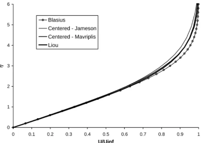
In opposition to Jameson and Mavriplis’ artificial dissipation model, Mavriplis (1990) model does not contain the time step in the dissipation terms. Therefore, it does not present an influence of the time step on the steady-state solution such as observed in Fig. 7 for Jameson and Mavriplis’ model. A comparison between these two artificial dissipation models is presented in Fig. 8, in which the solution using Liou’s scheme is also included. In this figure one can see that the solution with Mavriplis’ model is in better agreement with the Blasius solution than the solution with Jameson and Mavriplis’ model. Moreover, the numerical experiments performed showed that the time step influence on the solution is negligible when Mavriplis’ model is used. This means that, with Jameson and Mavriplis’ model and even for the larger time steps, there is some influence of the time step on the steady state solution.
The solution for the laminar flat plate using Liou’s spatial discretization scheme is also presented in Fig. 8, as already mentioned. This solution is very close to the solution with the centered spatial discretization scheme with Mavriplis’ artificial dissipation model. Hence, as the computational cost of Liou’s scheme is larger than that of the centered scheme, it is worthwhile to use the centered scheme in this case. Moreover, the influence of the time step on the steady-state numerical solution observed in the numerical experiments performed is also very small for the Liou (1996) scheme.
0 1 2 3 4 5 6
0 0.1 0.2 0.3 0.4 0.5 0.6 0.7 0.8 0.9 1
U/Uinf
η
Blasius
Centered - Jameson Centered - Mavriplis
Liou
Figure 8. Comparison of the spatial discretization procedure effect on the flat plate numerical solution (M∞ = 0.3 and Rel = 1.0 × 10
5
).
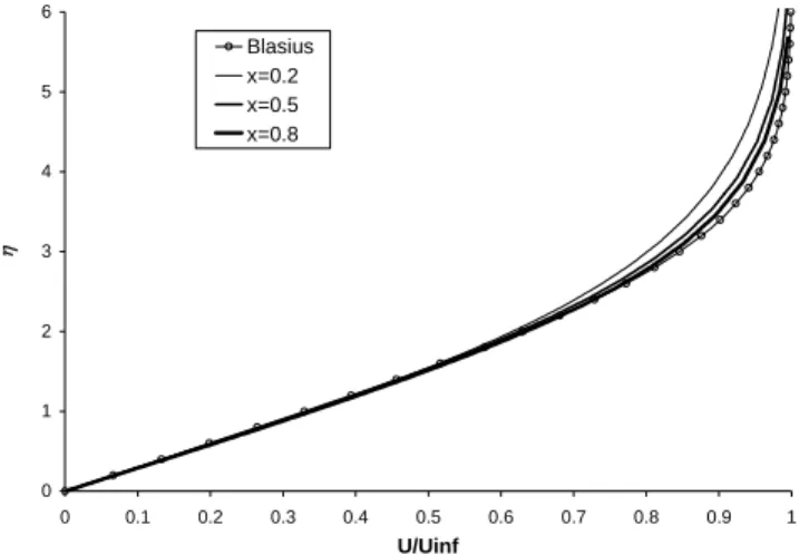
The Blasius exact solution of the laminar flat plate problem (see, for instance, Schlichting, 1979) is a self-similar solution when the previously defined η variable is used. The numerical results, using
0 1 2 3 4 5 6
0 0.1 0.2 0.3 0.4 0.5 0.6 0.7 0.8 0.9 1
U/Uinf
η
Blasius x=0.2 x=0.5 x=0.8
Figure 9. Similarity on the flat plate numerical results (M∞ = 0.3 and
Rel = 1.0 × 10
5
).
Flat plate results were also obtained for turbulent cases. The comparisons that will be shown in the forthcoming paragraphs will present results with both turbulence closure models implemented. In order to validate these models, a comparison of the numerical results with analytical solutions (Schlichting, 1979) was performed. For the case of a flat plate with zero pressure gradient, three different layers can be identified in the boundary layer close to the wall. The first layer is the viscous sublayer, where the turbulence is damped by the presence of the wall and, therefore, the laminar or molecular viscosity dominates. The second layer is a transition layer, or buffer layer. Finally, the third layer is the log layer, where the turbulence effects dominate the laminar effects.
The velocity profile in the viscous sublayer can be written as (Schlichting, 1979)
+
= y u
u
* , (29)
where
w w
u
ρ τ
= *
, (30)
and
ν ρ τ d y
w w
=
+ . (31)
In the log layer, the velocity profile is
5 ln 5 . 2
* = +
+
y u
u
, (32)
where the constants in the previous equation were obtained from experimental results(Schlichting, 1979).
The numerical results obtained with the Baldwin and Barth turbulence closure model and Liou’s scheme are presented in Fig. 10. In this figure the dimensionless velocity profiles for three different stations along the plate are presented, namely at 0.2, 0.5 and 0.8 plate lengths from the plate leading edge. It is evident from the figure that there is a very good agreement between the computational and analytical results. One can also observe in the figure that the velocity profiles at the different stations are
self-similar and, as for the laminar case, the best results are obtained for the stations farther from the plate leading edge.
0 5 10 15 20 25
0.1 1 10 100 1000
y+
U/
U*
Visc. sublayer Log law Numerical x = 0.2 Numerical x = 0.5 Numerical x = 0.8
Figure 10. Comparison of the numerical results using the Baldwin and Barth model with the analytical solution for the turbulent flat plate (M∞ = 0.3 and Rel = 2.0 × 10
6
).
A similar comparison to the one presented in Fig. 10 is shown in Fig. 11 for the Spalart and Allmaras turbulence closure model. Using this model, there is also a good agreement between the numerical and the analytical results, although it is not as good as the one observed with the Baldwin and Barth model results. Nevertheless, the results are still very good and the Spalart and Allmaras model is also used quite frequently in aerodynamic applications.
0 5 10 15 20 25
0.1 1 10 100 1000
y+
U/U*
Visc. sublayer Log law Numerical x = 0.2 Numerical x = 0.5 Numerical x = 0.8
Figure 11. Comparison of the numerical results using the Spalart and Allmaras model with the analytical solution for the turbulent flat plate (M∞ = 0.3 and Rel = 2.0 × 10
6
).
The results presented in this section were computed using the mesh shown in Fig. 3. For these cases, the y+ value for the first point of the mesh off the wall is slightly lower than 1. This value is adequate for both the Baldwin and Barth and the Spalart and Allmaras turbulence closure models, as discussed by the authors (Baldwin and Barth, 1990, Spalart and Allmaras, 1994). Moreover, no variation of the grid refinement was attempted as previous studies (Azevedo, Meneses and Fico, 1996) have indicated that the refinement adopted is adequate for the capture of turbulent boundary layers.
0 5 10 15 20 25 30 35
0.1 1 10 100 1000
y+
U/U*
Visc. sublayer Log law Numerical x = 0.2 Numerical x = 0.5 Numerical x = 0.8
Figure 12. Numerical results using the Baldwin and Barth model and the centered spatial discretization scheme (M∞ = 0.3 and Rel = 2.0 × 10
6
).
The capability developed is able to handle complex mesh topologies. For instance, Fig. 13 presents an example of a hybrid mesh for a flat plate and three agglomerated meshes that were obtained from this mesh. Again, one should note that only the (a) mesh in Fig. 13 has to be provided as input data. The other meshes are automatically generated by the agglomeration procedure. This topology represents a typical case for the treatment of viscous boundary layers in the proximity of solid walls, as quadrilaterals have been used near the wall and triangles away from it. It has the advantage of being capable of adequately capturing the viscous effects close to the body while reducing the number of points in the regions far from the body, where they are not needed.
(a) 6269 nodes, 13298 volumes
(b) 1848 nodes, 3435 volumes
Figure 13. Original (a) and agglomerated (b,c,d) hybrid meshes for the flat plate.
(c) 528 nodes, 928 volumes
(d) 157 nodes, 263 volumes
Figure 13. (Continued).
The computational results for the laminar flat plate obtained with the mesh shown in Fig. 13 are presented in Fig. 14. The centered spatial discretization scheme with Mavriplis’ artificial dissipation model was used in this case. The results with the same formulation but with the quadrilateral mesh presented in Fig. 3 are also shown in Fig. 14, as well as the exact Blasius solution. The velocity profiles plotted in Fig. 14 correspond to a station in the middle of the plate. From this figure, one can see that the results with the hybrid mesh are almost identical to the results with the quadrilateral mesh, as expected. Moreover, as previously discussed, the computational results are in good agreement with the Blasius solution.
0 1 2 3 4 5 6
0 0.1 0.2 0.3 0.4 0.5 0.6 0.7 0.8 0.9 1
U/Uinf
η
Hybrid Mesh Quadrilateral Mesh Blasius
Figure 14. Comparison of velocity profiles for the laminar flow over a flat plate using hybrid and quadrilateral unstructured meshes (M∞ = 0.3 and
Rel = 1.0 × 10
5
).
Conclusions
that can be made in order to reduce the computational costs of the multigrid procedure.
Laminar viscous flow over a 2-D flat plate was used to validate the implemented capability. Studies of the various parameters affecting the multigrid acceleration performance were undertaken with the objective of determining optimal numerical parameter combinations. The results obtained show a significant improvement in convergence in comparison with the case without the use of the multigrid procedure. Among the combinations tested, the best set of numerical parameters consists of 4 coarse meshes, 1 pre- and 1 pos-sweep iterations on every grid level and 40 iterations on the coarsest grid level.
A preliminary validation of the implemented capability was performed using laminar and turbulent flat plate simulations. In both cases, a very good agreement was obtained with the experimental and analytical results. The numerical solutions were compared to the Blasius solution for the laminar case and to the viscous sublayer and log-layer for the turbulent case. The Baldwin and Barth as well as the Spalart and Allmaras turbulence closure models gave essentially the same results, but the Baldwin and Barth model provided a slightly better comparison with the analytical results. Moreover, an effect of the CFL number on the steady-state solution was observed when the centered scheme with Jameson and Mavriplis’ artificial dissipation model was used. This is due to the fact that the scaling terms in this model are inversely proportional to the time step. Nevertheless, when the centered scheme with Mavriplis’ artificial dissipation model, or the Liou scheme, was used, no such time step effect was observed. Furthermore, for the turbulent case using the centered scheme, the comparison with the analytical results was poorer than the comparison when the Liou scheme was used. This was observed with both the Jameson and the Mavriplis artificial dissipation models and it is an indication that these artificial dissipation models introduce too much dissipation in this case, which is not observed with Liou’s scheme as it has its inherent artificial dissipation.
The increased flexibility provided by the use of unstructured grids was demonstrated with the use of hybrid meshes. The hybrid meshes have the advantage of being capable of adequately capturing the viscous effects close to the body while reducing the number of points in the regions far from the body, where they are not needed. Laminar flat plate results obtained in a hybrid mesh were identical to the ones obtained with a conventional quadrilateral mesh.
Acknowledgments
The authors gratefully acknowledge the partial support of Conselho Nacional de Desenvolvimento Científico e Tecnológico
(CNPq) under the Integrated Project Research Grant No. 522413/96-0.
References
Azevedo, J.L.F., and Korzenowski, H., 1998, “Comparison of Unstructured Grid Finite Volume Methods for Cold Gas Hypersonic Flow Simulations”, AIAA Paper No. 98-2629, Proceedings of the 16th AIAA Applied Aerodynamics Conference, Albuquerque, New Mexico, pp. 447-463.
Azevedo, J.L.F., Menezes, J.C.L., and Fico, N.G.C.R., Jr., 1996, “Accurate Turbulent Calculations of Transonic Launch Vehicle Flows,” AIAA Paper No. 96-2484-CP, Proceedings of the 14th AIAA Applied Aerodynamics Conference, Part 2, New Orleans, LA, pp. 841-851.
Baldwin, B.S., and Barth, T.J., 1990, “A One-Equation Turbulence Transport Model for High Reynolds Number Wall-Bounded Flows,” NASA TM-102847.
Barth, T.J., and Jespersen, D.C., 1989, “The Design and Application of Upwind Schemes on Unstructured Meshes”, AIAA Paper No. 89-0366, 27th AIAA Aerospace Sciences Meeting, Reno, NV.
Brandt, A, 1977, “Multi-level Adaptive Solutions to Boundary Value Problems”, Mathematics of Computation, Vol. 21, pp. 333-390.
Jameson, A., and Mavriplis, D.J., 1986, “Finite Volume Solution of the Two-Dimensional Euler Equations on a Regular Triangular Mesh”, AIAA Journal, Vol. 24, No. 4, pp. 611-618.
Liou, M.-S., 1996, “A Sequel to AUSM: AUSM+”, Journal of Computational Physics, Vol. 129, No. 2, pp. 364-382.
Mavriplis, D.J., 1988, “Multigrid Solution of the Two-Dimensional Euler Equations on Unstructured Triangular Meshes”, AIAA Journal, Vol. 26, No. 7, pp. 824-831.
Mavriplis, D.J., 1990, “Accurate Multigrid Solution of the Euler Equations on Unstructured and Adaptive Meshes”, AIAA Journal, Vol. 28, No. 2, pp. 213-221.
Mavriplis, D.J., and Jameson, A., 1990, “Multigrid Solution of the Navier-Stokes Equations on Triangular Meshes”, AIAA Journal, Vol. 28, No. 8, pp. 1415-1425.
Mavriplis, D.J., and Venkatakrishnan, V., 1994, “Agglomeration Multigrid for Viscous Turbulent Flows”, AIAA Paper No. 94-2332, Proceedings of the 25th AIAA Fluid Dynamics Conference, Colorado Springs, CO.
Schlichting, H., 1979, “Boundary Layer Theory”, McGraw-Hill, New York.
Spalart, P.R., and Allmaras, S.R. , 1994, “A One-equation Turbulence Model for Aerodynamic Flows,” La Recherche Aérospatiale, No. 1, pp. 5-21.
Strauss, D., and Azevedo, J.L.F., 2001, “Unstructured Multigrid Simulations of Axisymmetric Inviscid Launch Vehicle Flows,” AIAA Paper No. 2001-2476, 19th AIAA Applied Aerodynamics Conference, Anaheim, CA.
van Leer, B. , 1979, “Towards the Ultimate Conservative Difference Scheme. V. A Second-Order Sequel to Godunov's Method”, Journal of Computational Physics, Vol. 32, No. 1, pp. 101-136.
Venkatakrishnan, V., 1995, “Convergence to Steady State Solutions of the Euler Equations on Unstructured Grids with Limiters”, Journal of Computational Physics, Vol. 118, pp. 120-130.