J. Braz. Soc. Mech. Sci. & Eng. vol.33 número4

 

Carlos Duque-Daza

c.a.duque-daza@warwick.ac.uk Universidad Nacional de Colombia Department of Mechanical Engineering 111321 Bogotá, Colombia

Duncan Lockerby

d.a.lockerby@warwick.ac.uk University of Warwick Fluid Dynamics Research Centre School of Engineering CV4 7AL Coventry, UK

Carlos Galeano

chgaleanou@unal.edu.co Universidad Nacional de Colombia Department of Mechanical Engineering 111321 Bogotá, Colombia

Numerical Solution of the

Falkner-Skan Equation Using Third-Order and

High-Order-Compact Finite Difference

Schemes

We present a computational study of the solution of the Falkner-Skan equation (a third-order boundary value problem arising in boundary-layer theory) using high-third-order and high-order-compact finite differences schemes. There are a number of previously reported solution approaches that adopt a reduced-order system of equations, and numerical methods such as: shooting, Taylor series, Runge-Kutta and other semi-analytic methods. Interestingly, though, methods that solve the original non-reduced third-order equation directly are absent from the literature. Two high-order schemes are presented using both explicit (third-order) and implicit compact- difference (fourth-order) formulations on a semi-infinite domain; to our knowledge this is the first time that high-order finite difference schemes are presented to find numerical solutions to the non-reduced-order Falkner- Skan equation directly. This approach maintains the simplicity of Taylor-series coefficient matching methods, avoiding complicated numerical algorithms, and in turn presents valuable information about the numerical behaviour of the equation. The accuracy and effectiveness of this approach is established by comparison with published data for accelerating, constant and decelerating flows; excellent agreement is observed. In general, the numerical behaviour of formulations that seek an optimum physical domain size (for a given computational grid) is discussed. Based on new insight into such methods, an alternative optimisation procedure is proposed that should increase the range of initial seed points for which convergence can be achieved.

Keywords: laminar boundary layer, similarity analysis, high-order-compact finite differences

Introduction1

The Falkner-Skan equation, originally derived in 1931, Falkner and Skan (1931), is of central importance to the fluid mechanics of wall-bounded viscous flows. It is derived from the two-dimensional incompressible Navier-Stokes equations for a one-sided bounded flow using a similarity analysis (see Cebeci and Bradshaw (1977)) and its solution describes the form of an external laminar boundary layer in the presence of an adverse or favourable streamwise pressure gradient. Despite the apparent simplicity of the Falkner-Skan equation (a one-dimensional ordinary differential equation) solving it accurately can be fraught with difficulty; these problems mainly stem from its non-linearity and third-degree order. There are some examples of analytical solutions to the Falkner-Skan equations for special cases (see, e.g., Fang and Zhang (2008) and Magyari and Keller (2000)), but most studies have focused either on demonstrating a solution’s existence and uniqueness or finding a numerical/computational solution for particular boundary-layer conditions.

Results for solution existence and uniqueness to the Falkner-Skan equation can be found in Rosenhead (1963), Weyl (1942), Hartman (1972) and Tam (1970). In some of these works, ranges of validity for the boundary-layer parameters and similarity variable are established (see, e.g., Pade (2003)). More recently, Yang (2008) presents a non-existence result that places upper and lower bounds on, in essence, the non-dimensional wall shear stress. However, despite the amount of effort dedicated to this problem, this two-point boundary value problem still lacks a general closed-form solution, and as such, numerical treatments are the most common and valuable route for its study and solution.

Paper received 25 October 2010. Paper accepted 21 June 2011. Technical Editor: Fernando Rochinha

A raft of computational approaches and methodologies have been presented for the solution of the FS equation, see for example Hartree (1937), Asaithambii (1997), Asaithambi (1998, 2004b, 2005), Abbasbandy (2007), Alizadeh et al. (2009) and Zhang and Chen (2009). The most widely used and ‘classical’ approach to numerical solution is to reduce the boundary value problem to an initial value problem via a shooting method (see Cebeci and Bradshaw (1977); Cebeci and Keller (1971) for a thorough discussion). This involves prescribing known conditions at the wall boundaries along with an estimate for the velocity profile’s first derivative at the wall, which is successively refined until known far-field boundary conditions are satisfied. A recent development in shooting methods, presented by Liu et al. (2008), shows that, in fact, trial imposition of known boundary conditions is not necessary, as they can be formulated as unknowns of the solution procedure. Even so, shooting methods have the significant disadvantage of being more time consuming, as they essentially solve two or more initial value problems during each iteration, Asaithambi (1998), requiring a larger amount of computational nodes and memory capacity than other approaches. Another equally significant undesirable feature of shooting methods is their known convergence difficulties, which have to be overcome with modifications that significantly increase algorithm complexity, Asaithambi (2004b).

boundary-layer equations. However, in the works mentioned above, the original third-order boundary-value problem for the Falkner-Skan equation is either transformed into a reduced system of a first- and a second-order equation (to be solved by a coupled scheme) or solved using other complex numerical methods, some requiring additional adjustment coefficients to be calculated. In some cases, additional ‘fictitious’ end points are added, depending on the accur- acy and range of applicability of the particular numerical model proposed. Also, in addition to the mathematical complexity often involved, the numerical methods proposed tend to require significant computational time, as noted by Asaithambi (1998) and Salama and Mansour (2005b).

In the present work, we show how solutions to the original third-order Falkner-Skan boundary value problem (BVP) can be obtained using FDS, without the need for complex and involved mathematical algorithms, and at a relatively low programming and computational cost compared to other approaches of the same accuracy. Moreover, the approach presented in this paper is conceptually less complex, and at the same time able to obtain results with the same precision and bounding error limits as those previously reported. As such, the procedure is instructive and helpful, not just in terms of solutions to the Falkner-Skan equations, but to the direct application of FDS in cases where, normally, either a reduction of derivative order or an addition of fictitious end points would be required.

The paper is structured as follows. In Section 1 the Falkner-Skan equation is introduced and briefly discussed as a two-point boundary value problem, along with its characteristic boundary conditions. Section 2 details the modifications performed in the formulation of the Falkner-Skan equation in order to make it suitable to the numerical treatment of this paper. In Sections 3, 4 and 5, two different implementations are presented, the first using direct third- and fourth-order FDS, and the second using a methodology based on high-order-compact finite differences. In Sections 6 to 9 numerical results from the two schemes are presented and their accuracy discussed. Finally, in Section 10, some conclusions are drawn.

Nomenclature

f

= velocity function

f

= vector with the values of

f

g

= velocity function

h

= mesh size

J = Jacobian matrix of Y

N

= number of discrete points in the approximation

p

= fluid pressure

Re = Reynolds number of the air flow, Reynolds number

U = free-stream velocity

u

= x – component of velocity

v

= y – component of velocity Y = set of non-linear equations

Z = boundary condition function at

ζ

=1

Greek Symbols

α

= value of the second derivative of

f

at the wall

β

= dimensionless pressure-gradient parameter

ε

= convergence criterion

γ

= dimensionless pressure-gradient parameter

ρ

= fluid density

η

= dimensionless spatial variable

κ

= accuracy order of the approximation

ν

= kinematic viscosity

ξ

= dimensionless spatial variable

ψ

= Falkner-Skan conventional stream function

ζ

= dimensionless coordinate

Subscripts

∞

= relative to infinite

The Falkner-Skan Equation: a Two-Point Boundary-Value Problem

The Laminar boundary layers exhibiting self-similarity have been the subject of a large body of research as they provide useful insight into many key features of wall-bounded flows, as well as being the basis of approximate methods for calculating more complex, non-similar boundary-layer problems. The Falkner-Skan equation is obtained when a similarity analysis is performed on the two- dimensional, steady, incompressible Navier-Stokes equations for a one-sided bounded flow. The simplified continuity and momentum equations are as follows:

,

0

=

∂

+

∂

y

v

x

u

∂

∂

(1)

,

1

2 2

y

u

dx

dp

y

u

v

x

u

u

∂

∂

+

−

=

∂

+

∂

_ν

ρ

∂

∂

(2) where

x

is the streamwise and

y

is the wall-normal coordinate,

ρ

is the fluid density,

ν

is the kinematic viscosity,

p

is the fluid pressure, and

u

and

v

are the

x

−

and

y

−

components of velocity, respectively. For the boundary layer, these equations are subject to a simple set of boundary conditions:

at

y

=

0

,

u=0,

v

=

0

,

at

y

→

∞

,

u=U(x), (3) where U is the free-stream velocity, which is assumed to be a function of

x

. In this paper, only walls with non-transpiration and no-slip are considered, hence both components of velocity at the wall are zero. In order to perform a similarity analysis on Eqs. (1) and (2), Falkner and Skan (1931) proposed the following transformation:

,

y

x

U

ν

ξ

=

(4)

and an implicit dimensionless stream function

g

[

ξ

( )

x

,

y

]

such that:

[

x

,

ξ

(

x

,

y

)

]

U

(

x

)

ν

x

g

[

ξ

(

x

,

y

)

]

,

ψ

=

(5) where

ψ

is a conventional stream function used to define the two-dimensional velocity field:

y

u

∂

∂

=

ψ

and

x

v

∂

∂

−

  The two velocity components can be expressed in terms of

( )

ξ

g as follows:

g U

u

=

′

and

(

)

_,

2

1

2

1

g

dx

dU

U

x

g

g

x

U

v

=

ν

ξ

′

−

−

ν

(6)

with the prime symbol denoting a derivative with respect to

ξ

. Using Eq. (4), Eq. (5) and Eq. (6), the momentum equation (2) can be rewritten, after some algebraic manipulation, as:

,

0

1

2

1

2

2 2

3 3

=





























−

+

+

+

ξ

γ

ξ

γ

ξ

d

dg

d

g

d

g

d

g

d

₍₇₎

where

γ

is a dimensionless pressure-gradient parameter:

.

dx

dU

U

x

=

γ

Note, for zero pressure gradient, when y = 0, Eq. (7) reduces to the Blasius equation. The boundary conditions, Eq. (3), can now be rewritten using definitions for the velocity components given in Eq. (6):

at ξ =0, g=0, g′=0,

at

ξ

→∞, g′=1, (8) Hartree (1937) introduced an additional simplification to Eq. (7), defining the following linear transformation:

ξ

γ

η

2

1

+

=

and

,

2

1

g

f

=

γ

+

(9)

such that the Falkner-Skan equation, Eq. (7), can now be rewritten in its most common form:

, 0 1

2

2 2

3 3

=

   

   

     

− + +

η

β

η

η

d

df d

f d f d

f

d ₍₁₀₎

where

β

is the dimensionless pressure-gradient parameter:

.

1

2

+

=

γ

γ

β

(11)

The range of values for which

β

is physically meaningful is approximately −0.2≤β <∞ (corresponding to −0.09≤γ <∞. For 0≤β ≤2, the physical interpretation of the solution of the Falkner-Skan equation is the laminar boundary layer over an infinite wedge of vertex angle βπ (β=0 corresponds to the Blasius boundary layer).

Finally, using Hartree’s transformation, the boundary conditions are:

at

η

=0, f =0, f′=0, (12) at η→∞, f′=1, (13)

with the prime symbol denoting a derivative with respect to

η

. Note that transformations related to similarity analysis such as the one proposed by Falkner and Skan, herein presented, are particularly appropriate for two-dimensional boundary layers. If required, solutions for three-dimensional boundary layers can be obtained by a different transformation to that hereby discussed. Since the primary aim of these methodologies is to reduce the partial differential formulation to ordinary differential by reducing in one the number of spatial variables, then in the three-dimensional case, though slightly different, such transformation will produce a system of two ODEs instead of just one equation, like in the present case. A simple example of such transformation and the system obtained can be found in Hogberg and Henningson (1998).

Computational Domain Mapping and Problem Definition

The spatial variable

η

of Eq. (10) is defined in a semi-infinite physical domain [0,∞). For computational purposes different approaches to mapping or truncating the semi-finite domain have been presented in Asaithambi (2004b), Asaithambi (2005), Cebeci and Keller (1971) and Asaithambi (2004a). Asaithambi (2005) highlights problems relating to stability and convergence when attempting to directly solve the equation for the entire mapped semi-infinite domain. To avoid this, in the same way as in Asaithambi (1998, 2005); Abbasbandy (2007); Asaithambi (2004a); Salama and Man- sour (2005a), we identify an upper limit value of the variable

η

, denoted as

η

_∞, which allows a normalized finite computational domain to be established. This upper limit can be any value that is sufficiently greater than the (transformed) boundary layer thickness, at which point it is safe to assume the velocity profile asymptotically approaches the free stream limit. However, this upper limit on

η

is not known a priori, and must, therefore, be made part of the solution, as will be discussed later.

A common methodology of mapping the physical domain is to use

η

_∞ as a normalization parameter for

η

, and some relation between f and

η

_∞ for the normalization of f. Here though, f is not normalized, as there is no clear advantage for doing so, with only

η

being normalized using

η

_∞; this offers a simple and straightforward solution to the definition of the computational domain. The coordinate transformation adopted here is as follows:

. ∞ =

η

η

ζ

This maps the physical domain

[

0

,

η

_∞

]

to the fixed computational domain

[ ]

0,1. After some algebraic manipulation, Eq. (10) can be rewritten:

.

0

3 2

2 2

3 3

=

+













−

+

η

∞

_ζ

η

∞

β

_ζ

η

∞

β

ζ

d

df

d

f

d

f

d

f

d

₍₁₄₎

The boundary conditions are then:

As mentioned previously, the value

η

_∞ is not known a priori, and must be found as part of the computational solution. Given that η_∞ is significantly greater than the boundary-layer thickness (formally defined as the point where u = 0.99U), the function f can be assumed to behave asymptotically. As such we can replace the boundary condition on

f

′

, which requires the unknown value of

∞

η

, with a boundary condition on the second derivative, i.e.:

at ζ =1, _0. 2 2

= = ′′

ζ

d f d

f (17)

After solution, the value of

η

_∞ is found from the value of

f

′

. The second derivative of f is directly related to the wall shear stress, and is often used to characterize the solution obtained. Coppel (1960) showed that this value is a function of the parameter

b for b ≥ 0, and Veldman and Van der Vooren (1980) extended this result for b < 0. It is common to express this relationship as a boundary condition:

at ζ =0,

( )

_, 2 2

β α ζ = d

f

d ₍₁₈₎

where a is a function of b Coppel (1960).

Method of Solution

Numerical approaches to solving high-order derivates using FDS are limited by the large number of stencil points required for high accuracy. In the case of the Falkner-Skan equation, typically this is overcome by replacing the third-order boundary value problem with a set of two or more ordinary differential equations of a lower derivative order. This approach, though, has a number of difficulties; it requires a more complex algorithm and is somewhat expensive, computationally. Direct substitution of high-order accurate finite-difference expressions into the original third-order Falkner-Skan equation, Eq. (14), is conceptually, algorithmically and computationally simpler, but this has not been reported previously, presumably because of the lengthy algebraic manipulation arising from the discretization of the non-linear terms. In this paper, however, a direct replacement into the full third-order BVP has been achieved by taking advantage of modern symbolic manipulation software (here we have used MATHEMATICA®_).

The methodology of solution proposed is to generate a direct high-order accurate finite-difference representation of the function f and its derivatives. These expressions are substituted into the FS equations, which are solved using a Taylor-coefficient matching approach, for an initial guess of

η

_∞. The value of

f

′

at

1 =

ζ

is then used to provide a corrected value of

η

_∞, and the FS equation then resolved; the procedure is continued until a convergence criterion is met. What follows are the descriptions of two approaches that differ only in the finite-difference formula adopted: the first uses explicit third- and fourth-order accurate finite-difference stencils; the second uses an implicitly-defined high-order compact difference scheme. To the authors’ knowledge, neither has previously been applied directly to the third-order Falkner-Skan equation in its non-reduced form.

Formulation with an Explicit Third-Order Finite Difference Scheme

The first approach we consider is the use of high-order explicitly-defined difference formulae. For the first- and second-order derivatives of

f

, these are fourth-order accurate expressions, obtained using standard Taylor expansions, with 5-point stencils. However, in order to preserve a minimum accuracy of

O

(

h

3

)

, the third-order derivative was discretized using a 6-point stencil. This selection was chosen to experiment with fourth-order approximations for the equation’s non-linear terms, whereas for the linear term f ′′′ a lower (third) order approximation was used so as not to increase excessively the number of stencil points required. As such, this produces a formulation that is formally third-order accurate; however, as will be demonstrated later, in practice, it exhibits orders of accuracy between 3 and 4 (i.e.

( ) ( ) ( )

_h3 _{Oh Oh}4

O _≤ n _{≤ , where n is the effective order of}

accuracy).

If the computational domain

ζ

∈

[ ]

0,1 is divided into N−1 equally spaced subintervals using N discrete points, such that:

,

)

1

(

j

h

j

=

−

ζ

for a mesh with grid size

)

1

(

1

−

=

_N

h

, and if

f

_j

=

f

( )

ζ

_j , then the Falkner-Skan equation, Eq. (14), can be expressed in discrete form as follows:

( )

2 3

0

,

=

+

′

−

′′

+

′′′

η

∞ j j

η

∞

β

j

η

∞

β

j

f

f

f

f

(19) for j=1,2,...,N. The boundary conditions Eq. (15), Eq. (16) and Eq. (17) are then:

,

0

1

≡

f

f

₁

′

≡

0

,

f

_N

′

≡

η

_∞

,

f

_N

′′

≡

0

.

(20) In total there are N unknowns, i.e. N−1 values of

f

_j for

N

j=2,3,..., and the value of

η

_∞ as the N−th unknown. As mentioned above, the (N−1) values for

f

are solved for an initial predicted (or previous iteration) value of

η

_∞, which is subsequently corrected, and the procedure repeated, until convergence.

The 5-point centred-difference formulae used for the i−th point (assuming a grid of equal spacing h) are:

(

_{8 8}

)

( )

_,

12

1 4

2 1 1

2 f f f Oh

f h

f_i′= _i− − _i− + _i+ − _i+ +

(

_{16 30 16}

)

( )

_.

12

1 4

2 1 1

2

2 f f f f f Oh

h

f_i′′= − _i− + _i− − _i+ _i+ − _i+ +

For the third derivative, an asymmetric 6-point difference formula is used:

(

)

( )

3

3 2 1 1

2

3 10 14 7

4 1

h O

f f f f f

f h

f_{i i i i i i i}

+

− + −

+ − − =′

Equation (19) can be now expressed as follows:

,

0

12

8

8

12

16

30

16

4

7

14

10

3 2 2 1 1 2 2 2 1 1 2 3 3 2 1 1 2

≈

+













−

+

−

−













−

+

−

+

−

+













₋

₋

₊

₋

₊

₋

∞ + + − − ∞ − + − − ∞ + + + − −

β

η

β

η

η

h

f

f

f

f

h

f

f

f

f

f

f

h

f

f

f

f

f

f

i i i i i i i i i i i i i i i i (22)

with i=3,...,N−3. If the terms of order _O(_h3) _{or higher are} ignored, and Eq. (22) is expanded, a non-linear algebraic representation of Eq. (19) can be obtained. Letting

f

_i denote a vector with the values of f for a six-point stencil, pivoted at the i – th point, i.e.:

[

_{−2 −1 +1 +2 +3}

]

,

≡

i i i i i i

T

i

f

f

f

f

f

f

f

(23) then the non-linear algebraic expression can be expressed as follows:

(

;h,

β

,

η

_∞

)

=0,

Y_m f_m (24) for m=3,...,N−3, with

Y

_m being the

m

−

th

non-linear function of

f

_m and parameters

h

, β and

η

_∞.

Equation (24) provides

N

−5 equations for the N−1 variables

{ }

N j j

f

2

= . The four additional equations required for a complete

system are obtained using asymmetric difference representations of the boundary conditions given in Eq. (20). For the first-order derivative at the wall (or ‘leftmost’) boundary point, we use a fourth-order asymmetric 5-point difference formula:

(

)

( )

, 3 16 36 48 25 12 1 4 4 3 2 1 h O f f f f f h

fi i i i i i

+ − − − + − =

′ _{+ + + + (25)}

which combined with the first two boundary conditions in Eq. (20), and ignoring the terms of accuracy equal or higher than _O

( )

_h4 _, yields: . 0 12 3 16 36

48 2 − 3 + 4− 5 =

h f f f f (26) This can be expressed in a shorter form as:

, 0 ) ; ( ₃

1 h =

Y f (27) i.e., a function

Y

of the values in

f

₃. A second complementary equation is obtained by replacing the boundary conditions at ζ=0 directly into the Falkner-Skan equation, yielding:

.

0

3 1

′′

+′

η

∞

β

=

f

(28) A forward-sided 4th-order accuracy finite difference formula for the third derivative is given by:

( )

. 15 104 307 496 461 232 49 8 1 4 6 5 4 3 2 1

3 _{f f f} O h

f f f f h f i i i i i i i

i +

     − + − + − + − =′ ′′ + + + + + + After substitution into Eq. (28) (along with Eq. (20)), and

ignoring terms of equal or higher order than O

( )

h4 , it is possible to obtain: . 0 8 15 104 307 496 461 232 3 3 7 6 5 4 3

2− + − + − + =

∞

β

η

h f f f f f f (29) This can be expressed in a shorter form as a function

Y

of

f

₄ and parameters

h

, β and

η

_∞:

.

0

)

,

,

;

(

4

2

h

β

η

∞

=

Y

f

(30) The two remaining equations are obtained in a similar way at the free-stream (or ‘rightmost’) boundary point,

ζ

N=1.

A suitable asymmetric 5-point difference formula is:

( )

, 25 48 36 16 3 12 1 4 1 2 3 4 h O f f f f f h f N N N N N

N +

     + − + − = ′ − − −

− ₍₃₁₎

and using the third boundary condition in Eq. (20), and ignoring terms of _O

( )

_h4 _{and higher, yields:}

. 0 12 25 48 36 16

3 _{4 3 2 1}

= − + − + − ∞ − − − −

_η

h f f f f

f_{N N N N N (32)}

This can be rewritten as follows: , 0 ) , ; ( ₂

1 − ∞ =

− h

η

Y_N f_N (33) where the subindex N−1 has been assigned for convenience. The fourth, and final, additional equation is obtained by evaluating the Falkner-Skan equation at ζ =1, using the boundary conditions

∞ = ′

η

N

f and fN′′=0: .

0 = ′′′

N

f (34) The asymmetric backwards difference formula used to evaluate the third derivative is as follows:

( )

4 1 2 3 4 5 6

3 _{461 232 49}

496 307 104 15 8 1 h O f f f f f f f h f N N N N N N N

N +

     + − + − + − = ′′′ − − − − − −

and after substitution into Eq. (19), and some simplification, yields:

. 0 8 49 232 461 8 496 307 104 15 3 1 2 3 3 4 5 6 = + − + − + − − − − − − − h f f f h f f f f N N N N N N N (35)

,

0

)

;

(

*

3

2 −

=

−

h

Y

N

f

N (36)

where

f

_N*₋₃ is now defined as a vector with components f_k for

N N

k= −6,..., . Finally, the full system of

(

N−1

)

equations can be summarized:

(

)

( )

(

)

(

)

(

)

(

)



      

 

        

 

=

∞ − −

− −

∞ ∞

∞

η

η

β

η

β

η

β

, ;

; , , ;

, , ;

, , ;

2 1

* 3 2 4 2

3 1

h Y

h Y

h Y

h Y

Y

h

N N

N N

m m

f f f f

f

f Y

M M

(37)

with m=3,...,N−3. Now letting:

[

N N

]

T

f

f

f

f

1 2 −1

=

L

f

be a vector with the set of

N

−

1

variables or unknowns

{ }

N j j

f

₌₁, and consider the system Y as a non-linear system in

f

only. Then solving the non-linear system described by:

(

f

;

h

,

β

,

η

_∞

)

=

0

,

Y

(38) is equivalent to finding a solution to Eq. (19).

In this work an iterative process based on a Newton-type method has been used to solve Eq. (38). Any Newton-type method seeks a solution to a non-linear problem by solving a consecutive sequence of linearizations of the original problem. Letting

f

0 be an initial guess or ‘seed point’ (here seed point means a set of values for the unknows at an initial iteration or starting point) for the unknows

{ }

N

j j

f

1

= , and letting Y be at least once continuosly

differentiable in

f

(see Deuflhard (2006)), then a linearization with a general Newton-type method leads to:

( )

k k

( )

k,

J_Yf ∆f =−Yf _fk+1=_fk+∆_fk,

,... 1 , 0 =

k (39) where J_Y is the Jacobian matrix of Y in f defined by:

( )

,

1

2 1

1

2 1

    

 

    

 

∂ ∂ ∂

∂

∂ ∂ ∂

∂

=

− −

N N N

N

f Y f

Y

f Y f

Y J

L M O M

L

f

Y

(40)

which has a pentadiagonal-like structure, except for the first, second and penultimate rows. Each element of the central (N – 5) rows of

Y

J

(rows M = 3,…,N – 3) is defined by the appropriate derivatives of Eq. (24). For the other entries in

J

_Y, terms are calculated using appropriate derivatives of the functions

Y

₁,

Y

₂,

Y

_N−2 and

Y

_N−1 defined by Eq. (27), Eq. (30), Eq. (33) and Eq. (36) respectively (in the interest of brevity these expressions are omitted).

The system solved using Eq. (39) is the solution for an arbitrary

∞

η

. Letting l

∞

η

represent the l−th iteration value for

η

_∞,

f

k,l the

th

k− iteration of

f

for a given l

∞

η

, and

∆

f

k,l the increment required by the Newton-method correction within the k−th iteration for a given l

∞

η

, the system in Eq. (38) can be expressed as follows:

(

fk,l;h,

β

,

η

_∞l

)

=0.

Y (41) The general Newton-type method can now be restated as follows:

_J

( )

k,l k,l

(

k;_h, , l

)

, ∞ −

=

∆f Yf

β

η

f

Y

, , , ,

1l kl kl k

f f

f + = +∆ k=0,1,... (42) A convergence criterion is established, for a previously defined tolerance

ε

_f, on the norm of the correction:

,

,

f l k

_<

ε

∆

f

(43)

where

∞

⋅

denotes an

L

_∞-norm.

To find appropriate successive values for

η

_∞, a discrete form of the last boundary condition in Eq. (20) is employed as an auxiliary function. Using a 5-point backwards finite difference the condition is expressed as,

(

)

(

35 104 114 56 11

)

,

12 1

, ∞ = 2 N− N−1+ N−2− N−3+ N−4

l _{f f f f f}

h Zf

η

(44) with

f

l being the converged value of

f

k,l for a given

η

_∞l. In accordance with the asymptotic condition for the second derivative, this function Z must be zero at

η

∞

(

ζ

=1

)

. Since Z is an unknown implicit function of

η

_∞, finding the correct

η

_∞ is equivalent to finding the root of Z. Therefore, using a simple secant method as a root-finding algorithm, the process of finding

∞

η

can be written as:

.

1 1

1 l

l l

l l l l

Z

Z

Z

−

− ∞ ∞ ∞ +

∞

₋

−

−

=

η

η

η

η

(45)

This particular root-finding method was selected for its ease of implementation. A convergence criterion is defined, for a previously defined tolerance

ε

_Z, as follows:

(

l

,

)

_Z

.

Z

f

η

_∞

≤

ε

(46)

Formulation with Fourth-Order Compact Finite Differences

difference schemes. For the current case, schemes with 5-point stencils were selected for all the derivatives featuring in the Falkner-Skan equation Eq. (14). For a third-order derivative this is given by:

(

)

. 0 60 1 2 2 2 2 ) 7 ( 4 2 1 1 2 3 1 1 = + − + − + ′′′ +′ ′′ + ′′′ + − − + + − i i i i i i i i f h f f f f h f f f

This scheme is accurate to fourth-order accuracy with a 5-point stencil, as compared to that adopted in the previous section, which used a 6-point stencil to provide a third-order accurate approximation. Ignoring terms of order greater than or equal to h4 or derivatives greater than 6th order, the scheme can be simplified to:

(

2 2

)

0.

2 2 2 1 1 2 3 1 1 = − + − + ′′′ +′ ′′ + ′′′ + + − − + − i i i i i i i f f f f h f f f (47)

The Falkner-Skan equation Eq. (19) can be used to obtain the third-order derivative at an arbitrary computational point

i

using standard difference expressions for the first and second derivative. Evaluating this derivative at points i−1,

i

and i+1 (with standard symmetric and asymmetric differences, preserving the overall accuracy and 5-point stencil), allows substitution into the implicit Eq. (47) leading to:

(

2 2

)

0,

2 4 12 11 20 6 4 12 3 10 18 6 12 16 30 16 2 12 8 8 2 12 4 6 20 11 12 6 18 10 3 2 1 1 2 3 3 2 2 1 1 2 1 2 2 1 1 2 2 2 1 1 2 2 1 1 2 2 2 1 1 2 1 2 2 1 1 2 ≈ − + − + −      _{− + + − +} −      − + − + + +      − + − + − −       − + − +       − + + − −      − − + − + + + − − ∞ + + − − + ∞ + + − − ∞ + + − − ∞ + + − − ∞ + + − − − ∞ + + − − ∞ i i i i i i i i i i i i i i i i i i i i i i i i i i i i i i i i i i i i f f f f h h f f f f f f h f f f f f h f f f f f f h f f f f h f f f f f f h f f f f f β η η β η η β η η β η (48)

With i = 3,….N – 2 being a valid range for the discrete Eq. (48). Owing to the 5-point nature of the scheme, this only provides (N – 4) equations for the (N – 1) variables

{ }

N

j j

f

2

= . Here, though, Eq. (48)

only need to be applied for the (N – 5) points defined by i = 3,….N – 3, as there are sufficient boundary conditions from Section 2. These equations are conveniently expressed as:

(

_m;h,

β

,

η

_∞

)

=0,

m f

Y (49) for m=3,...,N−3, where Y_m is the m – th non-linear function of f_m

and parameters

h

, β and

η

_∞. The vector f_m is as defined in Eq. (23). In a similar manner to the method in Section 4, three of the additional equations required for a complete set are provided by

Eq. (27), Eq. (30) and Eq. (33). However, the fourth equation for this scheme was obtained by replacing the boundary condition Eq. (16) into Eq. (19) expressed at the node N, i.e.:

0 = ′′ +

′′′ ∞ N N

N f f

f

η

which using backwards formulas for

f

_N

′′

and

f

_N

′′′

of an appropriate accuracy (and ignoring terms of order greater than

h

4), becomes:

, 0 180 137 12 45 154 214 156 61 10 15 29 8 49 232 461 496 307 104 15 ) 6 ( 4 2 1 2 3 4 5 ) 7 ( 4 3 1 2 3 4 5 6 = + + − + − + − + + + − + − + − − − − − − ∞ − − − − − − N N N N N N N N N N N N N N N N f h h f f f f f f f f h h f f f f f f f η (50) and completes the set of non-linear equations. This last relation can be written as,

(

* ; ,

)

0,

3

2 − ∞ =

− N h

η

N f

Y (51) where

f

_N*₋₃ represents a vector with seven grid points centered at

3 − =N

i , in a similar fashion to the definition given by Eq. (23). In this way, using Eq. (27), Eq. (30), Eq. (33), Eq. (49) and Eq. (51), a non-linear system of (N – 1) unknowns with (N – 1) equations can be written as follows:

(

)

( )

(

)

(

)

(

)

(

)

,

,

;

,

;

,

,

;

,

,

;

;

,

,

;

2 1 * 3 2 4 2 3 1













































=

∞ − − ∞ − − ∞ ∞ ∞

η

η

η

β

η

β

η

β

h

Y

h

Y

h

Y

h

Y

h

Y

h

N N N N m m

f

f

f

f

f

f

Y

M

M

(52)

where m=3,...,N−3. This non-linear system is solved for f and

∞

η

using the same method as detailed in Section 4.

Numerical Results

A large number of solutions to the Falkner-Skan equation have been reported in the literature for varying values of

β

(though physically-relevant solutions only exist for −0.19884 ≤ b ≤ 2.0). In such studies, it is common to use the value of the second derivative at the wall (denoted as α) as a means to evaluate the quality and accuracy of the solution:

, 0 2 2 = = η

η

α

d f d

which is directly related to the skin-friction coefficient,

(

)

.

Re

1

2

γ

_α

x f

Since, though, there is no general analytical solution, the accuracy of numerical solutions is commonly evaluated in an indirect way, without reference to a true value, by presenting results for α as a limit value to a given precision. The two schemes proposed herein were tested for nine values of b ranging from −0.1988 to 2.00, in accordance with the range of values having physical meaning: for decelerating flows up to the flow separation limit, −0.19884 ≤ b ≤ 0; for accelerating flows, 0 ≤ b ≤ 2.0; and for constant flows, b = 0.

The actual order of accuracy for each scheme, for each value of b, is inferred using a common stability analysis (see, e.g., Asaithambi (2005)). As the numerical method used in this work is of a Taylor-series coefficient matching type, the absolute error for α is related to the grid size as follows:

,

~

_α

κ

α

−

_h

≈

Ch

(53) where α~ is the true value,

α

_h the converged value for a grid size

h, C is a proportionality constant and κ is the accuracy order of the approximation, i.e. the remainder after the truncation of the Taylor series in the discrete formula.

If h₁, h₂ and h₃ are three different grid sizes related by:

, 2

1 2

h

h = , 2

2 3

h h =

the order of accuracy can be calculated from Eq. (53) as:

,

2

log

.

log

2 3

1 2













−

−

≈

h h

h h

α

α

α

α

κ

(54)

with

α

_h1 ,

α

_h2 ,

α

_h3 being the computed values of

α

for h₁, h₂

and 3h , respectively.

Results for Explicit Third-Order Finite Difference Scheme

The explicit finite difference scheme of Section 4 has been tested using four grid sizes: h = 0.004, h = 0.002, h = 0.00125 and h = 0.001. All numerical tests were performed using prescribed error limit εf =1×10−10 and

15 10 1× − =

z

ε , to define convergence. In all

cases, the initial guess for

η

_∞ was 0 ₌3.5

∞

η , though convergence times were fairly insensitive to this seed point, provided ∞ it wasn’t too large, as will be discussed later, and except for negative values of b. The initial guess for

f

was given by f_i0 η0ζ_i

5 . 0 _∞

= , with no other requirement for the distribution being observed; tests with nonlinear initial functions of

f

were performed, but there was no significant improvement in the quality of the solution or on the rate of convergence. For all cases reported in this paper the convergence of the inner loop (associated with

ε

_f for a fixed k

∞

η

) was reached after 5 - 7 iterations, on average; the convergence of the outer loop (associated with

ε

_z) took around 20 - 25 iterations, except for some negative values of b which typically required more iterations.

Results for h = 0.00125 and h = 0.002 are presented in Table 1, given to 6 significant figures, alongside values obtained by Salama and Mansour (2005b) and Asaithambi (2005, 2004a). The results obtained with the current explicit formulation are in almost exact agreement with those obtained in previous studies, in most cases coinciding up to 5 significant figures for the full range of b

considered. Figure 1 shows normalized velocity profiles obtained using the current explicit scheme, for select values of b, at a grid resolution of h = 0.00125. Visual inspection shows these profiles to be in close agreement with others presented in the literature, e.g., Salama and Mansour (2005b), Schlichting and Gersten (2000) and Cebeci and Bradshaw (1977). Close inspection of the data shows that for higher values of b, a smaller

η

_∞ produces an optimum solution, as noted in the literature (see, e.g., Asaithambi (2005); Salama and Mansour (2005b)).

Figure 1. Velocity profiles for accelerating, constant and decelerating flows.

Table 1. Values of αααα obtained using the current explicit scheme for varying b.

β Current (h = 0.002)

Current

(h = 0.00125) Salama and Mansour (2005b) Asaithambi (2004a) Asaithambi (2005) 2.0000 1.687221 1.687219 1.687218 1.687218 1.687218 1.0000 1.232588 1.232588 1.232588 1.232588 1.232589 0.5000 0.927680 0.927680 0.927680 0.927680 0.927680 0.0000 0.469600 0.469600 0.469600 0.469600 0.469600 -0.1000 0.319270 0.319270 0.319270 0.319269 0.319270

-0.1200 0.281760 0.281761 - 0.281759 -

Table 2. Numerical verification of order of accuracy of the current explicit scheme, κκκκ, for differentb.

β αh1 αh2 αh3 κ

2.0000 1.68724479 1.68722053 1.68721838 3.5 1.0000 1.23259213 1.23258805 1.23258770 3.6 0.5000 0.92767938 0.92767999 0.92768003 3.9 0.0000 0.46959871 0.46959986 0.46959997 3.3 -0.1000 0.31926893 0.31926967 0.31926975 3.3 -0.1200 0.28175959 0.28176044 0.28176051 3.5 -0.1500 0.21636074 0.21636132 0.21636140 3.0 -0.1800 0.12863536 0.12863611 0.12863621 3.0 -0.1988 0.00519723 0.00521583 0.00521790 3.2

In Table 2 results are presented for the numerical approximation/verification of the order of accuracy of the current explicit formulation, for each value of b. Results for h₁= 0.004, h₂= 0.002 and h₃= 0.001, are used within Eq. (54) to obtain

κ

, a numerical measure of the accuracy order. In this way, the explicit formulation is verified as being at least third-order accurate (and in a few cases the accuracy appears to be close to fourth order). A second branch of solutions exist in the range −0.1988≤β<0, generally known as the ‘lower branch’ solutions, whose results are also presented in Table 2. The present method has been able to reach

these other solutions with adjustments in the seed values of

η

_∞, still preserving the third-order of accuracy. However, results for these cases, where the velocity profiles (

f

′

) are more complex and have no physical interpretation, have been intentionally ommited.

Results for Implicit High-Order-Compact Scheme

The implicit compact difference scheme of Section 5 was tested using grid spacing ranging from h = 0.00025 to h = 0.01, as presented in Table 3. The numerical tests for this scheme were performed with the convergence criteria εf <1×10−10 and

15

10 1× − <

z

ε . In all cases the initial guess for

η

_∞ was

η

∞ =4.0, though, as in the explicit scheme, other seed values exhibited similar convergence rates. The initial profile for

f

was chosen as

i i

f0 η0ζ

5 . 0 _∞

= and since this initial guess had little influence on the results of the explicit scheme, no other initial profiles were considered. For the majority of cases for this scheme, the convergence of the inner loop ∞ (the one associated with

ε

_f for a fixed k

∞

η

) was reached after 5 - 7 iterations; and for the outer loop (associated with

ε

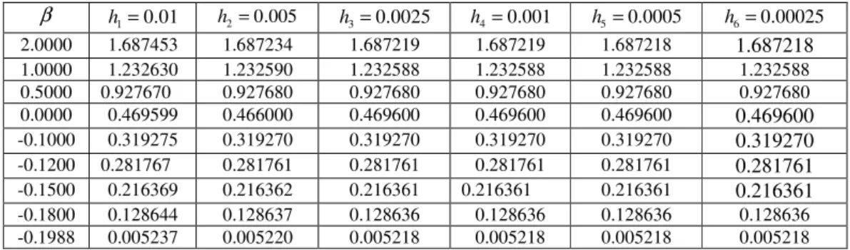
_z) around 17 - 20 iterations (though this was slightly greater for some negative values of β).

Table 3. Comparison of values obtained for αααα with the implicit scheme for different grid sizes.

β h1=0.01 h2=0.005 h3=0.0025 h4=0.001 h5=0.0005 h6=0.00025

2.0000 1.687453 1.687234 1.687219 1.687219 1.687218 1.687218 1.0000 1.232630 1.232590 1.232588 1.232588 1.232588 1.232588 0.5000 0.927670 0.927680 0.927680 0.927680 0.927680 0.927680 0.0000 0.469599 0.466000 0.469600 0.469600 0.469600 0.469600 -0.1000 0.319275 0.319270 0.319270 0.319270 0.319270 0.319270 -0.1200 0.281767 0.281761 0.281761 0.281761 0.281761 0.281761 -0.1500 0.216369 0.216362 0.216361 0.216361 0.216361 0.216361 -0.1800 0.128644 0.128637 0.128636 0.128636 0.128636 0.128636 -0.1988 0.005237 0.005220 0.005218 0.005218 0.005218 0.005218

Results obtained from the implicit compact-difference formulation for h = 0.00025 to h = 0.01 are presented in Table 3, with values given to six significant figures. It can be seen that results are converged (to the precision presented) for grids as large as h=0.001. In Table 4 the results of a numerical check on the order of accuracy of this implicit formulation (in accordance with Eq. (54)) are presented for varyingb. Two separate accuracy orders are calculated:

κ

₁ based on results for h1=0.01, h2=0.005 and

0025 . 0 3=

h ; and

κ

₂ based on results for h₄=0.001, 0005

. 0 5 =

h and h6=0.00025.

The tabulated values verify the fourth-order accuracy of the current implicit scheme. In addition to the basic set of numerical tests outlined above, we have performed a group of calculations to examine some numerical properties of the current scheme, such as bounds of solution validity and convergence characteristics. In the solution procedure described earlier, the value of

η

_∞ is refined in order to minimize the target function Z (i.e.

f

_∞

′′

). The function’s closeness to zero can be viewed as the degree to which the boundary

condition,

f

_∞

′′

=

0

, is satisfied; i.e., if

Z

≈

0

, then the solution can be assumed to be valid. This iterative refinement is the standard procedure for solution methods that use

η

_∞ for normalization, Asaithambi (1998, 2004b, 2005) and Abbasbandy (2007), though the reason and requirement for it has not previously been explicitly discussed. What has also been observed, but not explained, is that a relatively small initial (seed) value of

η

_∞ is required for convergence in these methods. In order to shed light on this optimization, in Fig. 2 we present the function

Z

(i.e.

f

_∞

′′

) evaluated for a range of

η

_∞ at different pressure gradient parameters; evidently there is a wide range of values for

η

_∞ that produce valid solutions under this criterion:

η

∞ ≥4 for

β

=

2

;

6 ≥ ∞

η

for

β

=

0

; and

η

_∞

≥

7

for

β

=−0.1988; and this is independent of the grid resolution. The form of the function

Z

is perhaps surprising, since it implies that provided an initial choice of

∞

Table 4. Numerical verification of order of accuracy for different b under explicit FDS.

b

κ

₁

κ

₂

2.0000 3.88 3.91 1.0000 4.04 4.54 0.5000 3.81 4.28 0.0000 6.31 3.80 -0.1000 3.93 4.20 -0.1200 3.97 3.59 -0.1500 4.02 3.48 -0.1800 3.96 4.39 -0.1988 4.38 5.09

Figure 2. Function Z

(

f′′

( )

η∞

)

for b = −0.1988 at different grid sizes, and for b = 0.0 and b = 2.0 for h = 2.5 E – 3.

However, although these solutions may be valid (in that they satisfy the far-field boundary condition on

f

′′

) they are not necessarily accurate in the boundary layer itself. This is because there is a trade-off, in terms of accuracy, between domain size (a larger one improving the physical model) and resolution throughout the boundary layer. Note, the grid spacing referred to in this paper (and in most previous works) is spacing/resolution on the normalized computational domain

ζ

or interval [0,1] and not the physical domain

η

, interval

[

0,η_∞

]

; when the computational grid resolution is fixed and

η

_∞ increases, the resolution in the physical domain (i.e.,

∆

η

) reduces, hence the requirement for an

η

_∞ optimization. A problem exists, though, due to the form of

Z

, which becomes very small, shallow, and numerically jagged, at high

∞

η

. This makes the minimum very difficult to find if a relatively high value of

η

_∞ is chosen as a seed point; this is why the range of usable initial values is rather restrictive. In Fig. 3 we plot α (i.e.,

) 0 (

f′′ ) against

η

_∞ for varying grid sizes (noting that constant grid size quoted is the computational grid, and is not equivalent to boundary-layer resolution). The values of α are normalized with respect to α*

, a result from the most refined simulation described above, and that which we will assume, for the purposes of discussing accuracy, to be the correct result in place of an analytical solution. As can be seen from the figure, for all the computational grids considered, the most accurate result (values approaching

1 *= α

α ) occurs at a relatively low value of

η

_∞, and that this

appears at a local minimum in the variation of

α

with

η

_∞. Progressively refined grids are plotted on the same graph and show a rapid convergence towards _*=1

α

α for larger

η

_∞. As an alternative to procedures that attempt to minimize

f

_∞

′′

, we propose that this local minimum in α be sought, which will allow a far greater range of initial seed points to be used and produce a more efficient and better-behaved optimization. The constrained optimization for the local minimum would be formulated, using KKT conditions, as:

∞ η

min

( )

0 2 2

=

∞

=

η

η

η

α

d

f

d

.

.

t

s

=

₀

∞

η

α

d

d

.

0

2 2

≤

−

∞

η

α

d

d

Figure 3. Variation of αααα (normalized with highly-resolved solution, αααα*) for varying physical domain extent, η_∞.

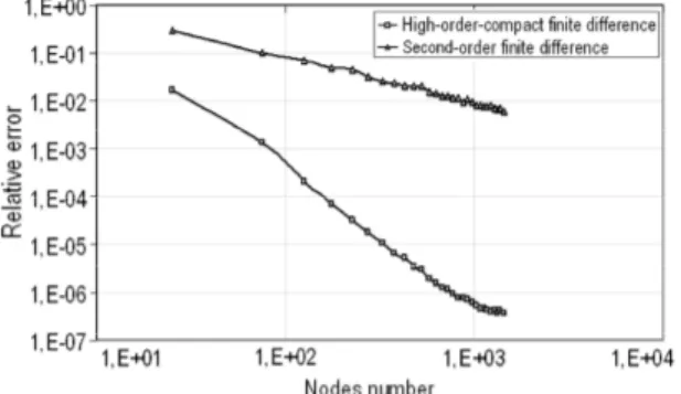
CPU Time and Accuracy

An additional indication of the numerical vantage attained using the high-order-compact scheme compared, particularly, against a conventional second-order finite differences stencil was sought by solving Eq. (14) for b = 0 with different number of nodes and, in both cases, gauging consumed computational time and numerical accuracy. Figure 4 shows a comparison of CPU time consumption per number of nodes for both schemes. Computational cost is nearly same, but with the technique proposed in this work exhibiting a clear slightly lower value. Considering that a smaller number of more intensive iterations were required in the high-order-compact scheme to achieve convergence for a prescribed convergence criterion, in contrast with that larger number of light iterations necessary for the second-order stencil, it is clear that such increased accuracy bring about a speed-up and, therefore, an improvement over traditional schemes.