Gustavo Meirelles Lima
limameirelles@gmail.com
Sandro M. M. de Lima e Silva
metrevel@unifei.edu.br Universidade Federal de Itajubá Instituto de Engenharia Mecânica 37500-903 Itajubá, Minas Gerais, Brazil
Thermal Effusivity Estimation of
Polymers in Time Domain
An accurate knowledge of thermophysical properties is very important, for example, to optimize the engineering design and the development of new materials for many applications. Thermal effusivity is a thermal property which presents an increasing importance in heat conduction problems. This property indicates the amount of thermal energy that a material is able to absorb. The estimation can be done by simulating a transient heat transfer model. In this case a one-dimensional semi-infinite thermal model is used. A resistance heater in contact with the sample generates a heat pulse. Variations of temperature and heat flux are measured simultaneously on the top surface of the sample. In this work, thermal effusivity is estimated in time domain through the minimization of the objective function, defined as the square difference between experimental and theoretical temperatures. The golden section technique is used for minimizing this objective function. A sensitivity analysis and a comparison between the semi-infinite and the finite models were also done to define the number of points to be used in the estimation. Measurements were carried out with three different polymers: polymethyl methacrylate, polyvinyl chloride and polyethylene. In all cases studied the results are in good agreement with literature. In addition, an uncertainty analysis is also presented.
Keywords: heat conduction, experimental methods, optimization, thermal effusivity
Introduction1
The knowledge about thermophysical properties of materials is even more necessary to make its correct application in engineering processes. Thermal conductivity, λ, thermal diffusivity, α, and thermal effusivity, b, are three important properties in heat conduction problems. Due to their importance, several methods have been developed to determine their values with accuracy and reliability. The methods which involve transient heat transfer stand out because they have an easy implementation, lower costs and shorter measurement time. In these methods a signal is generated, usually an impulse or a periodic function or a step-function, on the surface of the sample. The variations of temperature and heat flux are used to calculate the property. Blackwell (1954) presented the hot wire technique to measure thermal conductivity. A wire used as heater and temperature sensor is inserted inside the sample. A heat pulse is generated and the heat flux and temperature variations are measured. A disadvantage is that it is a destructive method because a hole has to be made in the sample. Also, it cannot be used in metals because of the thermal contact resistance and the short time for measurement. This method presents good results for insulation materials. Santos et al. (2004) and Carvalho et al. (2006) used it to measure thermal conductivity of polymers. To measure thermal diffusivity, Parker et al. (1961) developed the flash method. Since then it has been used several times and received improvements, as made by Sheindlin et al. (1998) and Min, Blumm and Lindemann (2007). Additionally, it is the most used method to measure thermal diffusivity of different kinds of materials. As an example, Iguchi, Santos and Gregório (2007) measured α of polymers and Blumm, Lindemann and Min (2007) measured α of water and ethylene glycol. The method consists in generating a high intensity energy pulse in a short time on the top surface of a thin sample. The variations of temperature are measured in the bottom face. Using a temperature versus time curve the thermal diffusivity can be calculated. The photoacoustic techniques have widely been used to measure thermal effusivity. These techniques can be used in many kinds of materials, including liquids, as in the work of Dadarlat et al. (2008). As shown by Benedetto and Spagnolo (1988), the technique
Paper received 11 March 2010. Paper accepted 10 August 2011. Technical Editor: Horácio Vielmo
is based on the measurement of sound wave intensity or phase. These waves are generated by any type of radiation absorbed by the material. A microphone is used to detect them. Generally, the radiation source is a light beam. To avoid the reflection, the surface of the sample must be opaque with a black paint with known thermal properties. The aforementioned techniques are restricted to laboratorial experiments.
Gustavo Meirelles Lima and Sandro M. M. de Lima e Silva
Nomenclature
B = thermal effusivity (W s1/2 K-1 m-2)
F = objective function (K²) L = sample thickness (m)
n = number of points used in estimation Sb = sensitivity coefficient (m² K² W-1 s-1/2)
t = time (s)
T = theoretical temperature (K) T0 = initial temperature (K)
Te = experimental temperature (K)
Ub = thermal effusivity uncertainty
Udata = data acquisition system uncertainty
Ue = experimental temperature uncertainty
UH.F. = heat flux uncertainty
UH.T. = heat flux transducer uncertainty
Unum = numerical uncertainty
Uobj = objective function uncertainty
UR = thermal contact resistance uncertainty
Utheo = theoretical temperature uncertainty
Utherm = thermocouple uncertainty
x = dimension (m) Greek Symbols
α = thermal diffusivity (m² s-1) λ = thermal conductivity (W m-1 K-1)
φ = heat flux (W m-2)
φ1(t) = heat flux measured (W m-2)
Subscripts
b =relative to thermal effusivity data = relative to data acquisition system e = relative to experimental measurement H.F. = relative to heat flux
H.T. = relative to heat transducer num = relative to numerical solution obj = relative to objective function R = relative to thermal contact resistance theo = relative to theoretical temperature therm = relative to thermocouple
0 = relative to initial time
1 = relative to frontal surface
Formulation of the Problem
Semi-infinite thermal model
The one-dimensional thermal model used is presented in Fig. 1. A semi-infinite solid is subjected to a heat flux on the top surface. The temperature measurement is on the same surface.
Figure 1. Semi-infinite sample subjected to a heat flux.
In this case, the heat diffusion problem can be described as:
2
2 1
T T
t
x α
∂ = ∂
∂
∂ (1)
The boundary and initial conditions are:
1 0
(0, ) ( )
x T
t t
x
ϕ λ ϕ
= ∂
= =
∂ (2)
0 ∞ → ) ,
(xt T
T x = (3)
0 ) 0 ,
(x T
T = (4)
where φ1(t) is the heat flux measured on the sample surface and T0 is
the initial temperature.
Several methods can be used to solve Eqs. (1)-(4) in order to obtain the temperature solution. For example, Green’s functions– GFs (Beck et al., 1992) and Laplace Transform (Özisik, 1993) are classical methods that can be used. In this work the GFs were chosen because a lot of problems are solved using this method. The same GFs for a given geometry and a given set of homogeneous boundary conditions is a building block of the temperature distribution resulting from: (a) space variable initial temperature distribution, (b) time- and space-variable boundary conditions, and (c) time- and space-variable volume and energy generation. Many GFs have been derived and are tabulated in Beck et al. (1992), so the derivation of GF may be omitted in many cases. Two and three-dimensional GFs can be found for transient cases by simple multiplication of one-dimensional GFs for the rectangular coordinate system for most boundary conditions, etc. In this sense the solution of the temperature problem presented in Eqs. (1)-(4) was obtained by using GFs solution for one-dimensional rectangular coordinates as (Beck et al., 1992).
τ
τ
λ
τ
φ
α
τ
d
x
t
x
G
dx
x
F
x
t
x
G
t
x
T
X t
L
x X
)
,'
,
(
)
(
'
)
'
(
).
0
,'
,
(
)
,
(
20 0
1 0 '
20
∫
∫
= =
+
=
(5)
where α is the thermal diffusivity, λ is the thermal conductivity and
F(x’) is the initial temperature distribution. The GF GX20 was found
in Beck et al. (1992) as:
2 / 1
20(0,t0,τ)=[πα(t−τ)]−
GX (6)
After some manipulations, the solution of temperature on the top surface T(0,t) of a semi-infinite medium can be written as:
∫
− − +=
t
d t
b T t T
0
1 2 / 1 2
1
0 . ( ) . ( )
. 1 )
, 0
( τ φ τ τ
π (7)
2 1
α λ =
b (8)
Equation (7) may be used to approximate the transient temperature response of a finite solid, such as a thick slab. This equation was solved numerically by the trapezoid rule method (Ruggiero and Lopes, 1996).
Thermal effusivity estimation
The thermal effusivity is estimated by minimizing an objective function. This function is defined as the square difference between experimental, Te, and theoretical, T, temperatures, defined as:
∑
= − = n
i
e i T i
T F
1
2 )] ( ) (
[ (9)
where n is the number of points used. To minimize the objective function (Eq. (9)), the Golden Section method (Vanderplaats, 2005) is used to determine the thermal effusivity.
Definition of the number of points used
A sensitivity analysis and a comparison between the semi-infinite and the finite models were done in order to choose the number of points n to be used in the estimation procedure. Values of thermal effusivity from literature were used to carry out these analyses. The values for PVC were obtained from Larbi Youcef et al. (2010), for PMMA from Roger et al. (1995), and for PVC from Jannot and Meukam (2004) (Table 1).
Table 1. Literature values used in the sensitivity analysis and in the comparison between semi-infinite and finite models.
Sample b (W s1/2 K-1 m-2)
PVC 408
PMMA 566
PE 888.6
Sensitivity analysis
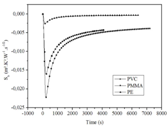
The sensitivity coefficient, Sb, is defined as the first derivative of
the temperature (Eq. (7)) with respect to the b parameter. The trapezoid rule method (Ruggiero and Lopes, 1996) was used to solve Eq. (10) numerically by using the experimental data of the heat flux φ1(t) and the reference values of b (Table 1).
∫
− − −= =
t
b t d
b db dT S
0
1 2 / 1 2
1
2. . ( ) . ( )
1 τ φ τ τ
π (10)
Equation (10) shows that Sb depends on the heat flux, the value
of b, and the time steps. Figure 2 shows the behavior of Sb for each
sample. It can be observed in this figure that for PE, Sb becomes
constant for times higher than 2000 s. In Fig. 2, a little contribution is given to the estimation procedure for times higher than 2640 s for PVC and 3500 s for PMMA. PVC presents the highest values of Sb
in Fig. 2. This happens because PVC has the smaller value of b and the smaller time step.
Figure 2. Sensitivity coefficients related to b for PMMA, PVC, and PE.
Comparison between semi-infinite and finite models
As already mentioned, the semi-infinite model must be used for the determination of b. In this work, the samples used are finite with a thickness of L = 50 mm. However, under certain conditions of time, the thermal behavior of a finite medium of thickness L can be considered identical to the semi-infinite medium (Beck et al., 1992). In addition, this behavior tends to be the same when the thickness and heat diffusion time are short. In order to verify this condition, a comparison between a finite model and a semi-infinite model is done for the calculated temperatures on the top surface. The finite model was given by a one-dimensional model with heat flux imposed on the top surface and insulation on the other surface (Fig. 3). For this case the heat diffusion (Eq. (1)) was used with the following boundary and initial conditions:
1 0
(0, ) ( )
x T
t t
x
ϕ λ ϕ
= ∂
= =
∂ (11)
( , ) 0
T L t x
∂ =
∂ (12)
0 ) 0 ,
(x T
T = (13)
Figure 3. Finite thermal model.
Gustavo Meirelles Lima and Sandro M. M. de Lima e Silva
sample, the higher the temperature for this model. This discrepancy happens only when the heater is on and it will be considered in the uncertainty analysis presented forward. In Fig. 4, it can be seen that for times higher than the values mentioned before for PVC, PMMA, and PE the finite model can not be considered semi-infinite.
Figure 4. Difference between finite and semi-infinite models.
Thermal Contact Resistance Influence
In heat conduction problems involving compound systems, in which the conduction occurs from a material to another, the thermal contact between them has great importance. Usually, a perfect thermal contact is assumed, but this does not occur in practice due to lack of flatness, the roughness of the samples, and the insertion of sensors such as thermocouples. These spaces are occupied by air, which causes a drop in temperature on the surface of the sample. So heat transfer occurs through the real contact area and the gaps. To determine the influence of thermal contact resistance in the experiments, an air layer of 0.01 mm thick between the transducer and the sample, as shown in Fig. 5, was simulated. Lima e Silva (2000) showed that on center of the heat transducer and the surrounding area, heat transfer can be considered one-dimensional.
Figure 5. Model adopted to analyze thermal contact resistance influence.
To determine the influence of the air layer, the temperatures on the surface of the transducer and the sample were compared (Fig. 6a). These temperatures were calculated for PVC (thermal effusivity from Table 1) by using experimental data of heat flux. Figure 6a shows that the difference between these temperatures increased with the rise of heat flux. However, for an air layer of only 0.01 mm the largest difference found was only 0.103°C (Fig. 6b). It represents an error of only 0.32%. So the effect of thermal contact resistance can be despised in thermal effusivity estimation. In addition, to reduce the contact resistance the heat transducer is placed under pressure with a thermal paste.
-1000 0 1000 2000 3000 4000 5000 6000 7000 8000 24
26 28 30 32 34
T
em
pe
ra
tu
re
(
°C
)
Time (s)
Sample Transducer
a)
-1000 0 1000 2000 3000 4000 5000 6000 7000 8000 0,00
0,02 0,04 0,06 0,08 0,10 0,12
D
if
fe
re
nc
e
(°
C
)
Time (s)
b)
Figure 6. a) Temperature evolution on the heat transducer and on the PVC sample; b) Difference between temperatures on the heat transducer and on the sample.
Experimental Procedure
AWG). This thermocouple was calibrated in a portable calibration bath ERTCO with a stability of ± 0.01ºC. The thermocouple was attached on the side of the heat transducer with the same thermal grease previously mentioned. Weights were used on the top of the isolated assembly to improve the contact between the components. Signs of heat flux and temperature are acquired by an acquisition system HP Series 75000 controlled by a computer. The sensors were attached on the middle of the sample. In Fig. 7, an oven which does not control the temperature was only used to minimize the convection influence and the variation of the ambient temperature over the sample. The sample was all isolated and Lima e Silva (2000) showed that for these conditions the convection can be neglected.
Figure 7. Scheme of the experimental apparatus.
Results
Table 2 shows the number of experiments carried out, the time interval of acquisition, and the number of points measured and used in the thermal effusivity estimation for PVC, PMMA, and PE samples. The difference between the procedures is due to the fact that the data were obtained from three different articles, for PE (Guimarães, Philippi and Thery, 1995), for PMMA (Lima e Silva, Duarte and Guimarães, 1998) and for PVC (Lima e Silva, Tiong and Guimarães, 2003). Since the equipment is the same, the authors made use of these experiments from the mentioned articles. A number of experiments were done in order to obtain reliable estimates of standard deviation and average of the data. According to the literature this number has to be at least 20 experiments (Holman, 2001).
Table 2. Number of experiments, time interval, points measured and used in the thermal effusivity estimation.
Sample Experiments Time Interval (s)
Total Points
Points Used
PVC 51 0.88 8192 3000
PMMA 42 1.00 4097 3500
PE 21 6.25 1030 320
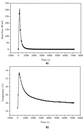
In all experiments the heat flux and the temperature evolution have the same behavior, as shown in Fig. 8. An impulse signal of heat flux imposed on the sample surface results in temperature increase. After this impulse, temperature begins to decrease.
-1000 0 1000 2000 3000 4000 5000 6000 7000 8000 0
50 100 150 200 250 300 350
H
ea
t
F
lu
x
(W
/m
²)
Time (s)
a)
-1000 0 1000 2000 3000 4000 5000 6000 7000 8000 24
26 28 30 32 34
T
em
pe
ra
tu
re
(
°C
)
Time (s)
b)
Figure 8. a) Heat flux evolution; b) Temperature evolution.
The results of thermal effusivity estimation are shown in Table 3. The values of b presented are an average of the values found in all experiments for each sample. The term “Difference” (Diff.) in Table 3 represents a comparison between b estimated in this work and b
from literature (Table 1). There is a significant variation in the values of b from literature for these materials. The “Standard Deviation” (SD) represents the difference observed among the experiments carried out with each sample. Table 3 presents different values of the Standard Deviation for each sample. The difference between them is explained by the higher number of experiments for PVC as well as the shortest time step.
Table 3. Average thermal effusivity, standard deviation and comparative difference with literature values.
Sample b
(W s1/2 K-1 m-2
)
Literature (W s1/2 K-1 m-2
) SD (%)
Diff. (%)
PVC 437 408 1.01 6.64
PMMA 522 566 2.44 7.77
PE 860 888.6 3.30 3.21
Uncertainty Analysis
Gustavo Meirelles Lima and Sandro M. M. de Lima e Silva
these signals. The hypothesis of linear propagation is used because the objective function is based on the difference between experimental and theoretical temperatures. The uncertainty for experimental temperature Ue is obtained from the uncertainties of
the data acquisition system UData, the thermocouple UTherm and the
thermal contact resistance UR.
2 2 2 2
R Therm Data
Exp U U U
U = + + (14)
The uncertainty of theoretical temperature is calculated from the uncertainties of the heat flux UH.F and the error of the numerical
calculus with the trapezoid rule UNum.
2 2
. . 2
Num F H
Theo U U
U = + (15)
The uncertainty of the heat flux can be determined from the uncertainties of the heat transducer UH.T. and the data acquisition
system UData.
2 . . 2 2
.
.F Data HT
H U U
U = + (16)
Combining Eqs. (14)-(16), the total uncertainty of the objective function can be calculated as:
2 2 2
. .
2 2 2
2
2 2.
Num R T H
Therm Data Theo
Exp Obj
U U U
U U U
U U
+ + +
+ =
+ =
(17)
The value for the uncertainty of the data acquisition system is based on an operation range between 20 and 35°C, auto-zero in position on with the Number of Power Line Cycle (NPLC) = 1, range of 125 mV with one hour of warm up.
% 00 . 1
= Data
U (18)
The estimation of the thermocouple uncertainty is based on the calibration of the thermocouple and on the maximum value of the measured temperature difference that was approximately 9.0°C. The thermocouple was calibrated in a bath calibrator (Thermometry Calibration System) with a maximum fluctuation of 0.1°C.
% 13 . 1
= Therm
U (19)
The uncertainty resultant of the thermal contact resistance is estimated with the maximum difference between the temperatures on the transducer and on the sample surface with an 0.01 thick air layer. This difference is 0.103°C, which results in an uncertainty of:
% 32 . 0
= R
U (20)
The uncertainties UThermand URare considered constant because
they represent the maximum uncertainties observed during the experiments.
The uncertainty of the heat transducer is estimated from its previous calibration considering a linear response, Uc, (Lima e
Silva, 2000), the uncertainties of tension, current and area of measurement. Tension and current were measured with a Goldstar digital multimeter with resolution of 0.01 V for the tension and 0.001 A for the current. The area was measured with a caliper with an uncertainty of 5 x 10-05 m.
(
2 2 2 2)
12 1.98%.
.T = c+ I + V + A =
H U U U U
U (21)
The numerical uncertainty is estimated taking into account the discrepancy previously presented (in the subsection Comparison between semi-finite and finite models) and the maximum difference between the temperature calculated by the trapezoid rule and the temperature calculated analytically (Lima e Silva, Duarte and Guimarães, 1998). This difference is 0.152°C, so the maximum uncertainty was estimated as:
% 47 . 0
= Num
U (22)
Substituting Eqs. (18)-(22) in Eq. (17), the uncertainty for the objective function is:
% 74 . 2
= Obj
U (23)
An analysis of propagation errors shows that the uncertainty in the original data propagates in a conservative way, and the total uncertainty of the thermal effusivity was found to be:
% 74 . 2
= = Obj
b U
U (24)
In this work there are inherent bias errors due to the limitations of theoretical model and the uncertainty in the experiment values. The samples were considered homogeneous and heat flux unidirectional. In addition, the thermal property was considered temperature independent. It can be observed that the uncertainty value estimated for the thermal property is a qualitative value and it is in agreement with the values found in the literature. This value of
Ub can be used as a reference value.
Conclusions
This work presented a non-destructive method for thermal characterization of a conductive system. It allows an in situ
measurement, which is important for engineering operations. The implementation of the system requires the sensors to measure the heat flux and temperature only on the top surface of the material. The thermal contact resistance can be more troublesome for in situ
measurements due to the irregularities on the surface. To reduce this effect, a thermal grease of high thermal conductivity can be used. The method presented good results to estimate the thermal effusivity of three different polymers using experimental data. These materials have low thermal conductivity and they can be assumed a semi-infinite medium. Differently from many authors who used the frequency domain, the thermal effusivity here was estimated in time domain. There are several advantages of using time domain, as for example, it is easier to estimate temperature dependent thermophysical properties than it is in the frequency domain.
There is no restriction to use this technique for materials of thermal conductivity higher than 2 W/m.K. Nevertheless, to use this technique for these materials, it is necessary that the sample present large thickness and the experiment time be short. This procedure must be used to respect the hypothesis of a semi-infinite medium.
Acknowledgements
References
Antczak, E., Chauchois, A., Defer, D. and Duthoit, B., 2003, “Characterization of the Thermal Effusivity of a Partially Saturated soil by the Inverse Method in the Frequency Domain”, Applied Thermal Engineering, Vol. 23, pp. 1525-1536.
Antczak, E., Defer, D., Elaoami, M., Chauchois, A. and Duthoit, B., 2007, “Monitoring and Thermal Characterization of Cement Matrix Materials Using Non-Destructive Testing”, NDT&E International, Vol. 40, pp. 428-438.
Beck, J.V., Cole, K.D., Haji-Sheikh, A. and Litkouhi, B., 1992, “Heat Conduction Using Green’s Functions”, Washington D.C., Hemisphere Publishing Corporation, 552 p.
Benedetto, G. and Spagnolo, R., 1988, “Photoacoustic Measurement of the Thermal Effusivity of Solids”, Applied Physics A: Solids and Surface, Vol. 46, pp. 169-172.
Blackwell, J.H., 1954, “Transient-Flow Method for Determination of Thermal Constants for Insulating Materials in Bulk”, Journal of Applied Physics, Vol. 25, pp. 137-144.
Blumm, J., Lindemann, A. and Min, S., 2007, “Thermal Characterization of Liquids and Pastes Using the Flash Technique”,
Thermochimica Acta, Vol. 455, pp. 26-29.
Carvalho, G., Pereira, F.R., Ramos, V.D., Costa, H.M. e Almeida, F.L. L., 2006, “Otimização do Cálculo de Condutividade Térmica em Polímeros”, in: V Congresso Brasileiro de Análise Térmica e Calorimetria, Poços de Caldas – MG (In Portuguese).
Coment E., Batsale J.C., Ladevie B. and Battaglia J.L., 2002, “A Simple Device for Determining Thermal Effusivity of Thin Plates”, High Temperatures – High Pressures, Vol. 34, pp. 627-637.
Crawford, R.J., 1998, “Plastics Engineering”, Butterworth-Heinemann, 3rd, 352 p.
Dadarlat D., Neamtu C., Houriez N., Delenclos S., Longuemart S. and Sahraoui A.H., 2008, “Photopyroelectric Measurement of Thermal Effusivity of Liquids by Sample’s Thickness Scan”, The European Physical Journal Special Topics, Vol. 153, pp. 115-118.
Defer D., Antczak E. and Duthoit B., 2001, “Measurement of Low Thermal Effusivity of Building Materials Using the Thermal Impedance Method”, Measurement Science and Technology, Vol. 12, pp. 549-556.
Guimarães, G., Philippi, P.C. and Thery P., 1995, “Use of Parameters Estimation Method in the Frequency Domain for the Simultaneous Estimation of Thermal Diffusivity and Conductivity”, Review of Scientific Instruments, Vol. 66, pp. 2582-2588.
Holman, J.P., 2001, “Experimental Methods for Engineers”, 7th ed.,
McGraw-Hill Book Company, New York, 720 p.
Iguchi, C.Y., Santos, W.N. and Gregório Jr., R., 2007, “Determination of Thermal Properties of Pyroelectric Polymers, Copolymers and Blends by the Laser Flash Technique”, Polymer Testing, Vol. 26, pp. 788-792.
Jannot, Y. and Meukam, P., 2004, “Simplified Estimation Method for the Determination of the Thermal Effusivity and Thermal Conductivity using a Low Cost Hot Trip”, Meas. Sci. Technol, Vol. 15, No. 9, pp. 1932-1938.
Krapez J.C., 2000, “Thermal Effusivity Profile Characterization from Pulse Photothermal Data”, Journal of Applied Physics, Vol. 87, pp. 4514-4524. Larbi Youcef, M.H.A., Ibos, L., Feuillet, V., Balcon, P., Candau, Y. and Filloux, A., 2010, “Diagnostic of Insulated Building Walls of Old Restored
Constructions Using Active Infrared Thermography”, 10th International
Conference on Quantitative Infrared Thermography, Québec, Canada. Leclerq, D. and Thery, P., 1983, “Apparatus for Simultaneous Temperature and Heat-flow Measurements under Transient Conditions”,
Review of Scientific Instruments, Vol. 54, pp. 374-380.
Lima e Silva, S.M.M., Duarte, M.A.V. and Guimarães, G. 1998, “A Correlation Function for Thermal Properties Estimation Applied to a Large Thickness Sample with a Single Surface”, Review of Scientific Instruments, Vol. 69, pp. 3290-3297.
Lima e Silva, S.M.M., 2000, “Experimental Techniques Development for Determining Thermal Diffusivity and Thermal Conductivity of Non-Metallic Materials Using Only one Active Surface”, Doctorate Thesis, (In Portuguese), Federal University of Uberlandia, Uberlandia, M.G., Brazil, 130 p.
Lima e Silva, S.M.M., Ong, T.H. and Guimarães, G, 2003, “Thermal Properties Estimation of Polymers Using Only One Active Surface”, Journal of the Brazilian Society of Mechanical Sciences and Engineering, Vol. 25, pp. 9-14.
Lima e Silva, S.M.M and Lima e Silva A.L.F., 2010, “Estimation of Thermal Effusivity of Polymers Using the Thermal Impedance Method”,
Latin American Applied Reseearch, Vol. 40, pp. 67-73.
Miller, M.S. and Kotlar A.J., 1991, “Technique for Measuring Thermal Diffusivity/Conductivity of Small Thermal-Insulator Specimens”, Review of Scientific Instruments, Vol. 64, pp. 2954-2960.
Min, S., Blumm, J. and Lindemann, A., 2007, “A New Laser Flash System for Measurement of the Thermophysical Properties”, Thermochimica Acta, Vol. 455, pp. 46-49.
Özisik, M.N., 1993, “Heat Conduction”, 2nd ed., John Wiley & Sons,
New York, 692p.
Parker, W.J., Jenkins, R.J., Butler, C.P. and Abbott, G.L., 1961, “Flash Method of Determining Thermal Diffusivity, Heat Capacity and Thermal Conductivity”, Journal of Applied Physics, Vol. 32, pp. 1679-1684.
Roger, J.P., Gleyzes, P., El Rhaleb, H., Fournier, D. and Boccara, A.C., 1995, “Optical and Thermal Characterization of Coatings”, Thin Solid Films, Vol. 261, pp. 132-138.
Ruggiero, M.A. e Lopes, V.L.R., 1996, “Cálculo Numérico: Aspectos Teóricos e Computacionais”, Makron Books, 2a ed., 406 p. (In Portuguese).
Santos, W.N., Gregório, R., Mummery, P. and Wallwork, A., 2004, “Método do Fio Quente na Determinação das Propriedades Térmicas de Polímeros”,
Polímeros: Ciência e Tecnologia, Vol. 14, pp. 354-359 (In Portuguese). Sheindlin, M., Halton, D., Musella, M. and Ronchi, C., 1998, “Advances in the Use of Laser-Flash Techniques for Thermal Diffusivity Measurement”,
Review of Scientific Instruments, Vol. 69, pp. 1426-1436.
Taylor, J.R., 1997, “An Introduction to Error Analysis: The Study of Uncertainties in Physical Measurements”, University Science Books, 2nd ed.,
327 p.
Vanderplaats, G.N., 2005, “Numerical Optimization Techniques for Engineering Design”, Vanderplaats Research and Development Inc, 4th ed.,
USA, 466 p.