Andre L. Goldstein
andregold@fem.unicamp.br State University of Campinas – UNICAMP1School of Mechanical Engineering Department of Computational Mechanics – DMC Rua Mendeleyev, 200 13083-970 Campinas, SP, Brazil
Self-Tuning Multimodal Piezoelectric
Shunt Damping
Piezoelectric shunt damping is a well known structural vibration control technique that consists in connecting an electrical circuit to a piezoelectric transducer attached to the structure. In the case of a resonant shunt, the network consisting of an inductor-resistor network when combined with the capacitive nature of the piezoelectric transducer impedance can be designed to act as a tuned vibration absorber. This paper discusses a method for the design and online adaptation of multimodal piezoelectric resonant shunts. The method presented in this work is different from previously multi-modal shunting methods (“current blocking” and “current flowing”) and implements the shunting network with a reduced number of discrete electrical components besides allowing for online tuning of the shunting parameters. The mathematical model of a structure with bonded piezoelectric transducers connected to a general electrical network is reviewed and the coupled equations of motion of a simply supported beam with piezoelectric elements and passive shunt networks are derived. The design of the multimodal shunt network is presented based on passive filter synthesis methods. The multimodal self tuning piezoelectric damper is demonstrated experimentallyas a two-mode system applied to add damping to a cantilevered beam.
Keywords: piezoelectric shunting, resonant shunt circuit, multimodal damping
Introduction1
In recent years there has been great interest in the use of piezoelectric materials to implement distributed actuators and sensors in active vibration control systems and so-called intelligent or smart structures. It has also been demonstrated that piezoelectric materials can be used passively to add damping to the structure. In this case, the piezoelectric element is used in combination with an electrical network, usually called a ‘shunt network’ that can be designed to add damping to the structure. The use of different kind of shunts for vibration control and damping was reviewed by Lesieutre (1998). Among the several types of electric networks that can be used to shunt piezoelectric transducers, the inductive shunt that results in a resonant LC network has received most attention in the recent years. This network can be tuned so that the behavior of the resulting system is analogous to that of a mechanical vibration absorber (Hagood and von Flotow, 1991). If a resistor is added to the shunt, resulting in a LCR network, the device acts like a damped vibration absorber that achieves the reduction of the resonant mechanical response of the target mode by replacing it with two damped modes. Since the pioneering work of Forward (1979), which introduced and demonstrated the concept of inductive shunting, several advances have been made. Edberg et al. (1992) introduced the use of variable synthetic inductors where the inductance is changed by varying a resistor in the network. In their work a two-mode resonant network was demonstrated, but few theoretical results were presented regarding the design of the shunt network parameters. Multimodal shunting was also investigated by Viana and Steffen (2006), who discussed the modeling of modeling of piezoelectric patches coupled to shunt network including a review of the basics of resonant network topologies. In addition, the modeling of multi-degree-of-freedom mechanical system was presented as well as a design methodology for the multi-modal case, although it was assumed each PZT was shunted with a parallel network of resistor and inductor designed to control a specific structural mode. Browning and Wynn (1993) presented experimental results of the implementation of a multimode resonant shunting to reduce the broadband response of a plate. They used four piezoelectric elements positioned on the plate such as to target
This research work was performed during the author’s Ph.D. studies at Virginia Tech University’s Vibration and Acoustics Laboratory.
Paper received 29 March 2010. Paper accepted 28 July 2011. Technical Editor: Domingos Rade
twelve structural modes and each piezoelectric element was shunted by a network designed to damp three modes. The design of the network was accomplished by synthesizing the desired admittance function as a LC ladder circuit with floating inductors that are not suitable for implementation with synthetic inductors using operational amplifiers. Hollkamp (1994) also presented a method of an inductive piezoelectric shunting using a single piezoelectric element to damp multiple modes, however, no closed form solution for tuning was presented and the network parameters were determined by numerical optimization aiming at minimizing the weighted vibration energy. Experimental results were presented for two-mode device applied to a cantilever beam. Wu (1998, 1999) reported a method of implementing multi-mode shunt damping using a single piezoelectric element and provided closed form analytical expression to derive the network parameter values. The network proposed uses a parallel R–L branch for each mode to be controlled. The coupling between the individual parallel shunt networks was prevented with additional “current blocking” networks consisting of L-C parallel branches placed in series with each parallel R-L branch network. This scheme results in a large number of components that increases fast with the number of modes to be controlled. In Behrens et al. (2002), an alternative method to design a multi-mode piezoelectric shunting network was presented called the “current flowing” method, in contrast with the “current blocking” method presented by Wu (1996). In this method, additional series L-C branches are added in series with each L-R shunt branch. The “current flowing" shunt was studied theoretically and validated experimentally on two resonant structures. This approach requires a smaller number of components and requires no floating inductors when compared with the “current blocking” method.
J. of the Braz. Soc. of Mech. Sci. & Eng. Copyright 2011 by ABCM October-December 2011, Vol. XXXIII, No. 4 / 429
response of the system given by the voltage output of another piezoelectric element. The success of the control approach required that the system response data were filtered to include only a single vibration mode. Niederberger et al. (2004) and Fleming and Moheimani (2003) investigated an adaptive multi-modal piezoelectric shunt method that used the so-called synthetic impedance method, introduced in Fleming et al. (2002), which replaces simpler physical networks by a voltage-controlled current-source and a DSP system to implement the terminal impedance of an arbitrary shunt network.
In this work a method to design and implement a multi-mode self-tuning piezoelectric vibration absorber using physical networks is discussed. The method allows for a reduced total number of components and uses grounded inductors that can be implemented with synthetic inductors. First, a review of the theoretical modeling of a structure coupled to piezoelectric elements and general shunt electrical network is presented. Then, the procedure for designing a shunt network for damping multiple structural modes with a single piezoelectric element is shown, including the derivation of the state space equations of the shunt network. The method is illustrated with a worked out example of a two-mode shunt applied to cantilever beam. Finally, a method to implement the self-tuning of the multimodal shunt is introduced and the implementation of a self-tuning system is demonstrated experimentally.
Nomenclature
A = state dynamic matrix B = state input matrix
Cp = capacitance of the piezoelectric transducer cs = structural stiffness matrix
D = vectors of electrical displacements, [C/m2 ]
E = vectors of electrical field, [V/m]
e = piezoelectric material constant that relates voltage to stress f = vector of forces, [N]
K = stiffness matrix
Ke = kinetic energy
Lu = elastic differential operator Lϕ = eletrical differential operator
q = applied charge
Rs = strain rotation matrices RE = electrical field rotation matrices S = vector of material strains T = vector of material stresses, [N/m2] V = potential energy
We = electrical energy of the system Wm = virtual work due to magnetic terms W = work done by non-conservative forces w = mechanical displacements, [m]
YT = combined admittance of the shunt network and piezoelectric element capacitance
ϕ = scalar electrical potential ε = matrix of dielectric constants
Piezostructure Mathematical Model
In this section, a review of the piezostructure mathematical model is presented, following the derivation shown by Hagood et al. (1990). The equations of motion of the piezoelectric coupled electromechanical system are derived using a Rayleigh-Ritz formulation where the displacement and electric potential mode shapes are combined through the piezoelectric properties to form coupled equations of motion. This model includes the effects of the added mass and stiffness of the PZT patches bonded to the structure
that are important to predict the correct resonant frequencies for lightweight structures.
State-space model of the structure
The schematic of the structure considered is shown in Fig. 1, where the electrodes of piezoelectric element mounted on a beam are connected to an electrical circuit with impedance Z(s).
Figure 1. Schematic representation of a beam with piezoelectric element shunted to an external electrical circuit.
The derivation of the theoretical model of the beam structure starts with the generalized form of Hamilton’s principle for electromechanical system (Meirovitch, 1997):
[
]
∫
2 − + − + =1
0 t
t
m e
e V W W W dt
K δ
δ( ) (1)
where Ke is the kinetic energy, V is the potential energy, We is the electrical energy of the system, Wm is the virtual work due to magnetic terms which is negligible for piezoceramic materials. W is the work done by all other non-conservative forces.
Each of the terms above is defined as follows:
dv dv
K
p V
T p s
V T s
e =
∫
ρ w& w& +∫
ρ w& w&2 1 2
1
(2)
dv dv
V
p V
T
s V
T
∫
∫
+= S T S T
2 1 2
1
(3)
dv W
p V
T e =
∫
E D2 1
(4)
and
j nq
j j i nf
i
i x q
x
W δ δϕ
δ =
∑
⋅ −∑
⋅=
=1 1
) ( )
( w
f (5)
Where: w and fare the vectors of mechanical displacements and forces at location xj, respectively. qj and ϕj are the applied charge and scalar electrical potential at electrode j, respectively. S and T
are vectors of material strains and stresses, respectively. And D and
E are vectors of electrical displacements and electrical field, respectively.
The constitutive relation for the structure material is given as:
T = csS (6)
where csis the structural stiffness matrix. PZT
Shunt circuit
The constitutive relation for the piezoelectric can be written as (Hagood and von Flotow, 1991):
− = S E R R R R R R R R T D s E T E E s T s s T E E s T E c ε e ε (7)
where ε is the matrix of dielectric constants; e is the piezoelectric material constant that relates voltage to stress; Rs and RE are the appropriated rotation matrices
The superscript s means that the parameter was measured at constant strain, while E means that it was measured at constant electrical field. Now, the strain-displacement and field-potential relations are introduced as:
S = Luw(x) and E = Lϕϕ(x) = -∇ . ϕ(x) (8)
where Lu is the linear differential operator for the particular elasticity problem (Cook, 1981), Lϕ is the eletrical differential operator and ∇ is the gradient operator.
The displacement and potential are now expressed in terms of generalized coordinates ri(t) and vj(t) and assumed displacement and potential distributions (mode shapes) Ψ:
[
]
= ) ( : ) ( ) ( )... ( ) ( ) , ( t r t r x x x t x n rn r r 1 21 ψ ψ
ψ w (9)
[
]
= ) ( : ) ( ) ( )... ( ) ( ) , ( t v t v x x x t x n vn v v 1 21 ψ ψ
ψ
ϕ (10)
The assumed displacement and potential distributions need to obey respectively the geometric and prescribed voltage boundary conditions and also be differentiable to the order of the linear operators Lu or Lϕ.
Substituting the equations above into the expression for the Hamilton’s principle and taking the variations, after further manipulation it is possible to arrive at the actuator and sensor equations of the system:
f B Θv r K K r M
Ms p) ( s p) f
( + &&+ + − = (11)
q B v C r Θ q p
T + =
(12)
where the mass and stiffness matrices are given by the following volume integrals: dV x x s V r s T r
s =
∫
Ψ ( ) Ψ ( )M ρ (13)
dV x x p V r p T r
p =
∫
Ψ ( ) Ψ ( )M ρ (14)
dV x L x L s V r u s T r u
s =
∫
( Ψ ( )) c Ψ ( )K (15) dV x L c x L p V r u s E T s T r u
p=
∫
( Ψ ( )) R R ( Ψ ( ))K (16)
and the electromechanical coupling matrix is:
dV x L e x L p V v E t T s T r u
∫
= ( Ψ ( )) R R ( Ψ ( ))
Θ ϕ (17)
where the subscripts p and s mean that the integrals are performed over the piezoelectric material and over the structure respectively.
Writing Eq. (11) in state space form:
Du Cx y Bu Ax x + = + = & (18) where: + + − = − 0 K K M M I 0 A ) ( )
( s p 1 s p (19)
+ + = − − f p s p
s ) ( )
(M M Θ M M B
0 0
B 1 1 (20)
= r r x
& ,
= f v u (21)
The matrices C and D depend on the choice of observed inputs. The charge driven system can be obtained from the voltage driven case showed above by noting that Eq. (12) can be rewritten as:
q B C r Θ C
v=− p−1 T + p−1 q
(22)
Substituting this expression into Eq. (21) and rearranging gives:
u B x A x q r q
r = +
& (23)
u D x C
y r q
q + = (24) where: + −
= M− K ΘC−Θ 0 I 0
A
)
( p T
q 1 1 (25) = − − − )
( p q
f M ΘC B B
M
I 0
Bq 1 1 1 (26)
= q f u (27) and:
J. of the Braz. Soc. of Mech. Sci. & Eng. Copyright 2011 by ABCM October-December 2011, Vol. XXXIII, No. 4 / 431
State-space model of the structure with shunt electrical network
The shunt network can also be characterized by its state space model. The output of the model is the current flowing out of the piezoelectric electrodes, Ip, and the input are the voltages at the piezoelectric electrodes, vp. Following the terminology introduced by Hagood et al. (1990), a general state space model for the shunt network can be written as:
p el el el
el A x B v
x& = + (28)
p el el el
p C x D v
I = + (29)
This model can be coupled into the state space model given by Eqs. (23) and (24) observing that Ip, the current at the piezoelectric electrodes, is the derivative of the charge q and that vp is function of q and r. The augmented state space model including the shunt model can be written as:
sh sh sh sh
sh A x B u
x& = + (30)
sh sh sh sh
u D x C
y= + (31)
where:
=
el r
sh x
q x
x (32)
] [f
ush = (33)
− − =
− −
− −
− −
el q p T q el T p T q el
el q p T q el T p T q el
q p q
sh
A B C B B Θ C B B
C B C B D Θ C B D
B ΘC M A
A
1 1
1 1
1 1
0
) (
(34)
[
f]
shB M
B = −1
(35)
and the matrices Csh and Dsh depend again on the choice of observed outputs.
Shunt Network Design
In this section, the problem of choosing the appropriated electrical network configuration and component values of the shunt so as to apply damping to the target modes of vibration is discussed. Shunting networks are designed so that when connected to piezoelectric transducers bonded to the structure, the combined electrical impedance is high at the frequencies corresponding to the structural modes. Assuming that the piezoelectric transducer capacitance is known and using methods of network synthesis, it is possible to design the shunt network that has the required low electrical admittance at the target structural mode frequencies.
The derivation considers the design of a passive lossless L-C ladder network through passive filter synthesis techniques as presented for example by Chen (1986). The addition of damping can be made later by adding resistors in series with the inductors. In general, damping provided by resistor is an important parameter to optimize the shunt performance as discussed by Viana and Steffen
(2006) and Wu (1996). However, it is worth noticing that, in practice, due to the large inductance values usually required, the inductors are implemented using operational amplifiers. These synthetic inductors have an inherent resistance that sometimes can be larger than the ideal design value, leading to a non optimal design. In this work the design of a lossless network is assumed to simplify the synthesis procedure. The optimization of shunt parameters is an important research problem and is treated in detail by Steffen and Inman (1999) and Steffen et al. (2000).
The expression for the impedance of the L-C ladder network can be written based on the fact that the driving point impedance of a lossless network is a always a quotient of even to odd or odd to even polynomials (Chen, 1986).
)... )(
(
)... )(
)( (
2 2 2 2
1 2
2 3 2 2
2 2 2
1 2
1
p p
z z
z T
T
s s
s
s s
s H Y Z
ω ω
ω ω
ω
+ +
+ +
+ =
= (36)
In the expression above, ωzi and ωpi are respectively the frequency of the zeros and poles in radians per second that are specified before the synthesis. Note also that the poles and zeros of
ZT alternate along the jω axis and the poles and zeros frequencies of Eq. (36) are related by:
...
< < < <
≤ 1 1 2 2
0 ωz ωp ωz ωp
In the case of a shunting network, the expression for ZT is the combined shunt and piezoelectric impedance (Browning and Wynn, 1993):
YT= Yshunt + sCp
The shunt admittance alone is obtained by subtracting the capacitive impedance of the PZT Cp from the total impedance:
z z p z p T shunt
N N sC D sC Y
Y = − = − (37)
where Nz and Dz are, respectively, the numerator and denominator of Eq. (36).
This admittance function can be realized using the synthesis procedure that results in ladder networks known as Cauer II canonical form (Chen, 1986). This network configuration uses grounded inductors that are more appropriate for implementation with synthetic inductors. The process of obtaining Cauer II canonical form starts assuming that the desired electrical impedance is given by:
Z(s) = m(s)/n(s) (38)
Note that the polynomial m is assumed to be of higher degree than n, otherwise one would consider Y(s) = 1/Z(s) instead. The Cauer II canonical form requires that the numerator and denominator polynomials be arranged in ascending order of s:
1 1 3
3 1
2 2 2
2 0
− − − − + + +
+ +
+ + =
= k
k k k k k
s b s b s b
s a s a s a a s n
s m s Z
... ... )
( ) ( )
( (39)
... )
(
1 1
1 1
1 1
1 1
4 3 2 1
+ + + + =
s L s C s L s C s
Z (40)
The general ladder network that can realize this expression is shown in Fig. 2.
Figure 2. General ladder network obtained by the Cauer II synthesis.
Design example: two mode shunt network
Considering a two mode shunt network with two inductors the expression for electrical impedance is given by:
) )( (
) (
2 2 1 2
1 2 1
d s d s
n s ks D
N Y Z
z z T T
+ +
+ =
=
= (41)
where k is a real value to be determined, d1= (ωp1)2 , d2= (ωp2)2 and
n1= (ωn1)2.
The expression for the shunt electrical admittance is:
s kn ks
d d s kC n d d s k C
N N sC D sC Y Y
p p
z z p z p T shunt
) (
) (
1 3
2 1 2 1 2 1 4
1
+
+ −
+ + −
= −
= − =
(42)
If k is made equal to 1/Cp, Ys simplifies into:
ds cs
b as s n C s C
d d n d d s Y
p p
shunt
+ + = +
+ − +
= 32
1 3
2 1 1 2 1 2
1
1/ /
) (
(43)
where: a = d1 + d2 – n1, b = d1d2, c = 1/Cp andd = 1/Cpn1.
Now, writing as a continued fraction, the expression for the shunt electrical admittance becomes:
s (a-bc/d)/c s
d/(a-bc/d) s
b/d Yshunt
1 1
+ +
= (44)
The values of the inductors and the value of the capacitor are given by:
2 1 1 1
d d C
n L
p
= (45)
)] d d )n n d [(d C L
p 1 2 1 1 1 2 2
1 − − +
= (46)
p C n
d d n n d n d
C
+ − −
= 2
1
2 1 2 1 1 2 1 1
1 (47)
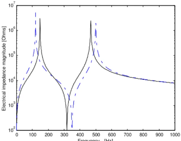
The electrical network that realizes this expansion is shown in Fig. 3. The electrical impedance of the shunt network above, using the parameters listed in Table 1, is plotted as the solid line in Fig. 4.
Note that the values of the electrical components computed with Eqs. (45) to (47) depend on the frequencies of the poles and zeros. These values are selected in the synthesis, with the values of the pole frequencies corresponding to the target resonance frequencies of the structure. Using the expressions for the component values derived above, each time the network is tuned to target different structural modes, it requires that new values be determined for all the components. This would make the implementation of a self-tuning shunt difficult, since it would be necessary to vary both the inductors and capacitors values.
Figure 3. Lossless electric network that implements two-mode shunt damping.
A method to tune the shunt network by varying only the values of the inductors while keeping the capacitor fixed can be implemented observing that the frequency of the zeros that occur between each pair of poles can be allowed to shift as the poles are shifted to follow the target frequencies without negative impact on the performance of the shunt. Then, an expression can be written to compute the values of the zero frequency n1 in terms of the values of the pole frequencies, the value of the capacitor C1 and of the piezoelectric capacitance Cp.
Table 1. Pole and Zeros Frequencies and Electrical Component Values.
Frequency of pole 1 148 Hz
Frequency of pole 2 469 Hz
Frequency of zero 300 Hz
PZT capacitance 24 nF
Value of inductor L1 19.71 H
Value of inductor L2 10.73 H
Value of capacitor C1 26.22 nF
Value of resistor R1 and R2 100 Ohms
For the example of a two-mode shunt network shown in Fig. 3, manipulation of Eq. (47) results in a second order equation that can be solved for n1:
0 2 1 2 1 1 1
2
1 C +Cp −n Cpd +Cpd +ddCp=
n( ) ( ) (48)
and
) (
) ( )
( ) (
p
p p p
p p
p
C C
C C C d d d C d C d C d C n
+
+ −
+ +
+ =
1
1 2 1 2 2 1 2
1 1
2
4
J. of the Braz. Soc. of Mech. Sci. & Eng. Copyright 2011 by ABCM October-December 2011, Vol. XXXIII, No. 4 / 433
Thus, it is possible to keep the capacitor value fixed and tune the network by selecting the required values of the poles and then computing the value of the zero using Eq. (49). Then, the required values of the inductors are computed using Eq. (45) and Eq. (46). The electrical impedance magnitude for the shunt network tuning modified to have poles at 120 Hz and 500 Hz is shown in as the dashed line in Fig. 4.
Figure 4. Electrical impedance magnitude for a two-mode shunt network. Solid line: tuning with poles at 148 Hz and 469 Hz; dashed line: new tuning with poles at 120 Hz and 500 Hz.
State-Space Model of the Shunt Network
In this section, the derivation of the shunt network state-space model matrices Ael, Bel, Cel and Del (Eqs. (28) and (29)) are presented. The details of the procedure can be found in Chen (1990). The shunt network is shown in Fig. 5(a), where voltage source V represents the PZT. Each element in the network is replaced by a line segment to obtain the linear graph model of the network. Then, an orientation represented geometrically by the edge-orientation arrows is assigned to each edge, resulting in the directed graph shown in Fig. 5.
(a) (b)
Figure 5. (a) Shunt network; (b) associated directed graph.
The edge e1 contains a voltage source and is added with the purpose of representing the PZT. Let ik and vk be the current and voltage of the edge ek (k = 1,2,…,6). In order to develop state equations for the system, a normal tree has to be selected. A tree of a directed graph is a connected subgraph that contains all the nodes of the graph, but no circuits. In this example, without lost of generality, the tree e1e3e4e6 is chosen. The KCL (Kirchhoff’s current law) and KVL (Kirchhoff’s voltage law) equations corresponding to the chosen tree are:
= − − − 0 0 0 0 1 0 0 0 1 0 0 1 0 0 1 0 0 0 1 0 0 1 0 0 0 1 1 1 6 4 3 1 5 2 i i i i i i (50) = − − − 0 0 0 0 1 1 0 1 1 1 1 1 1 0 6 4 3 1 5 2 v v v v v v (51)
The voltage-current equations of each element of the network are given by the expressions below:
v1 = vp (52)
v2 = L1 di2/dt (53)
i3 = v3/R1 (54)
i4 = C1 dv4/dt (55)
v5 = L2 di5/dt (56)
i6 = v6/R2 (57)
The state variables are chosen to be the capacitor voltage v4 and the inductor currents i2 and i5. Now, the goal is to express di2/dt, dv4/dt and di5/dt as functions of the voltage v4 and the currents i2 and i5. Substituting Eq. (52) to Eq. (57) into Eq. (50) and Eq. (51) results in: p v L L i i v L R L L R C i i v + − − − = 2 1 5 2 4 2 2 2 1 1 1 5 2 4 1 1 0 0 1 0 0 1 0 0 / / / / / / & & & (58)
The system output is the current going through the PZT, i.e., i1=Ip. It is given by:
[
]
− − = 5 2 4 1 1 0 i i vIp (59)
Hence the state-space matrices become:
− − − = 2 2 2 1 1 1 0 1 0 0 1 0 0 L R L L R C el / / / / A (60) = 2 1 1 1 0 L L el / / B (61)
0 100 200 300 400 500 600 700 800 900 1000 102 103 104 105 106 107
Frequency [Hz]
[
0 −1 −1]
= el
C (62)
0 = el
D (63)
Using the procedure described above, the complete mathematical model of the piezostructure connected to the shunt network is obtained. The method is applied to model a cantilever beam with a single piezoelectric patch bonded in the center of the beam and connected to a two-mode shunt tuned to the 2nd and 4th modes of the beam. The physical parameters of the beam and piezoelectric transducers are listed in Table 2. The acceleration response at the free end of the beam with and without the two-mode shunt is shown in Fig. 6.
Table 2. Physical parameters of cantilever beam and piezoelectric patch.
Aluminum beam PZT element
Length (mm) 300 72.4
Thickness (mm) 3.17 0.508
Width (mm) 35.6 35
Young’s Modulus (N/m2) 70 x 109 66 x 109
Density (kg/m3) 2700 7800
Capacitance (nF) --- 80
Piezoelectric strain
coefficient (m/V) --- 190 x 10
-12
Figure 6. Simultaneous damping of two modes with single PZT patch.
Experimental Implementation of Self-Tuning Shunts
The PZT elements used are the T120-A4E-602 from Piezo Systems, Inc. The beam used has a length of 300 mm, width of 35.6 mm and thickness equal to 3.17 mm. The dimensions of the beam and PZT parameters are summarized in Table 2. For the beam used in this experiment, the frequencies of the second and fourth modes are at 149 Hz and 468 Hz. The necessary inductance values are approximately 22.2 H and 11.3 H and using a 22nF capacitor. Due to the large inductance values necessary to implement the shunts network to damp modes at low frequencies, it is usual to use synthetic inductors using operational amplifiers. A common network configuration found in the literature is the so called gyrator filter (Horowitz and Hill, 1980) shown in Fig. 7. The effective input impedance of this network is given by:
2 4 3 1RR R sCR s
Zin( )= / (60)
By varying the value of one of the resistors, for example R3, using a potentiometer, the inductance of the network can be easily changed. In this work the two-channel, 256 positions digitally controlled variable resistor (VR) device, from Analog Devices was used. This device contains two independent variable resistors, each part consisting of a fixed resistor with a wiper contact controlled by a 10 bits word loaded into a controlling serial input register pin. The resistance of the wiper and the endpoints of the resistor have linear variation with respect to the code input. A control algorithm to perform the automatic tuning of the shunt network parameters was implemented using LabVIEW running in a PC host computer. The error signal from an accelerometer located at the tip of the beam is acquired and processed to identify the resonance frequency peaks of the structure. The identification of the resonant peak power and frequency is performed in the frequency domain by analyzing the auto-spectrum of the accelerometer output. A schematic of the experimental setup is shown in Fig. 8.
Figure 7. Synthetic inductor using operational amplifiers.
Figure 8. Experimental setup of self-tuning multi-modal piezoelectric shunting system.
The value of the piezoelectric element capacitance necessary for the tuning procedure was measured with a capacitance meter. Then, an initial tuning was performed using the expressions derived above to compute the inductance values necessary to tune the shunt to the target frequencies. Once the values of the inductors are determined, the resistor values required are evaluated and the digital potentiometers are set. After an initial tuning is performed the fine tuning of the shunt parameters is done using the fact that the addition of the shunted piezoelectric to the original system
0 100 200 300 400 500 600 700 800 900 1000 -100
-90 -80 -70 -60 -50 -40 -30
F
re
q
u
e
n
c
y
R
e
s
p
o
n
s
e
[
d
B
]
Frequenc y [Hz]
Cantilever B eam with S ingle P ZT and M ultiple S hunts
Semi-active auto-tuning shunt network Accelerometer
Computer with Data Acquisition Board and Lab VIEW Charge
Amplifier
Disturbance
Filter
Cantilever Beam
J. of the Braz. Soc. of Mech. Sci. & Eng. Copyright 2011 by ABCM October-December 2011, Vol. XXXIII, No. 4 / 435
transforms the original resonance peak in two damped peaks. For the optimal tuning condition the two damped resonances will have the same amplitude and the root mean squared (RMS) energy is minimized. For a sub optimal tuning condition, one of the new resultant peaks will have higher amplitude, as illustrated in Fig. 9. Observing the amplitudes of the resulting peaks after the shunting is applied allows determining how the value of inductance needs to be changed: if the peak is at a frequency higher than the original peak, the inductance has to be increased and vice versa. Note that in order for the self-tuning system to converge, the initial tuning has to be close enough to the pre-defined target frequencies so that the original resonance peaks are damped by shunt.
A fine tuning of the shunt parameters is performed through the minimization of the RMS energy in a frequency band centered on each resonance frequency. The procedure to find the optimal tuning consists of a simple line search, as the function to be minimized is unimodal over the closed interval around the resonant peak. The inductance of the shunt is varied by a step in an initial direction and the effect on the RMS energy is determined. If the effect of the change results in RMS energy increase, the direction of change is reversed. If the effect of the change results in RMS energy reduction, an additional step-change of smaller value is applied so that after a number of iterations the inductance values converge to the optimal values.
Figure 9. Resonant peak for optimal and sub-optimal tuning conditions.
In this experiment a two-mode shunt network was implemented in order to add damping to an aluminum cantilever excited by a PZT actuator bonded to the base of the beam. The shunt network was connected to single piezoelectric patch bonded midway along the beam. Clearly, the effectiveness of the shunted piezoelectric patch in damping structural modes depends on where the PZT element is attached to the structure and damping for certain structural modes can be achieved by placing the PZT elements on specific positions on the structure. Given the geometrical position of the PZT patch and the beam mode shapes, the 2nd and 4th vibration modes were chosen as target modes in the shunt design. The response at the accelerometer location before and after the shunting is applied is shown in Fig. 10. The reductions obtained are approximately 7 dB for the 2nd mode and 13 dB for the 4th mode. Note that the experimental results shown in Fig. 10 have good agreement with the predicted results shown in Fig. 6. The differences in the vibration amplitude reductions predicted numerically and measured experimentally can be explained for example by the inherent resistance of the synthetic inductor presented in the experiments and also by differences between the
numerical and experimental electromechanical coupling of the PZT patch and the beam structure.
Figure 10. Experimental results: damping of 2nd and 4th modes using self-tuning shunt.
Conclusions
In this work a procedure for the design and implementation of a self-tuning multimodal piezoelectric shunting damping system using a single piezoelectric element was presented. The theoretical modeling of a piezostructure connected to a shunt network was reviewed and multiple mode shunt design method based on passive filter synthesis techniques was demonstrated analytically. This multiple mode shunt network discussed has the advantage of implementing the multimodal shunting network with a minimal number of components when compared to “current blocking” and “current flowing” techniques. The design of a self-tuning shunt network was discussed and demonstrated experimentally. The inductors were implemented using synthetic inductors circuits based on using operational amplifiers that have their values modified by changing the values of a variable resistor, in this case a digitally controlled potentiometer. A tuning algorithm was introduced and implemented in LabView running on a PC computer. In the proposed method, the averaging of the auto-spectrum of the error signal required to reduce the measurement noise and increase the prediction accuracy of the resonant peaks and RMS energy made the algorithm convergence somewhat slow. However, the performance could be greatly improved by using a faster dedicated device. It is worth noting that, although in theory there is an optimal inductance and resistance values for the optimal tuning of the shunt, in practice the use of a synthetic inductor that has an inherent resistance made the use of an additional resistance not required. In practice, this results in a sub-optimal tuning condition, or the best possible performance with the given network implementation, as the control algorithm will always try to minimize the total energy of the resonant peak. In this work the error sensor was an accelerometer located near the tip of the beam. Future work can investigate the use of alternative error sensors such as an array of accelerometers to reduce total kinetic energy of the beam and shaped PVDF sensors for minimizing broadband radiated noise.
Acknowledgements
The author is grateful to the government funding agency Fundação de Amparo à Pesquisa de São Paulo, FAPESP, for the financial support to the present research work through process number 2009/10715-1. The author is also grateful to his Ph.D. advisor Chris R. Fuller.
400 450 500 550 600 650 700 -80
-75 -70 -65 -60 -55 -50 -45 -40 -35 -30
Frequency [Hz]
R
e
s
p
o
n
s
e
[
d
B
]
0 100 200 300 400 500 600 700 800 900 1000 -40
-30 -20 -10 0 10 20 30
Frequenc y [Hz ]
F
re
q
u
e
n
c
y
R
e
s
p
o
n
s
e
[
d
B
References
Behrens S., Moheimani S. O. R. and Fleming A. J., 2003, “Multiple
mode current flowing passive piezoelectric shunt controller”, Journal of
Sound and Vibration, Vol. 266, pp. 929-42.
Browning, D., Wynn, N., 1992, “Multiple-mode piezoelectric passive damping experiments for an elastic plate”, Proceedings of the 11th International Modal Analysis Conference.
Chen, W-K, 1990, “Linear Networks and Systems: Algorithms and Computer-Aided Implementations”, World Scientific Publishing Co., Inc.
Chen, W-K., 1986, “Passive and Active Filters: Theory and Implementations", John Wiley & Sons.
Cook, R.D., 1981, “Concepts and Applications of Finite Element Analysis”, Academic Press, New York, NY.
Forward, R.L., 1979, “Electronic Damping of Vibrations in Optical
Structures”, Applied Optics, Vol. 18, No. 5, pp.690-697.
Fleming, A.J and Moheimani, S.O.R, 2003, “Adaptive Piezoelectric
Shunt Damping”, Smart Materials and Structures, Vol. 12, pp. 36-48.
Edberg, D.L., Bicos, A.S, Fuller, C.M., Tracy, J.J. and Fechter, J.S., 1992, “Theoretical and Experimental Studies of a Truss Incorporating Active Members”, Journal of Intelligent Material Systems and Structures, Vol. 3, pp. 333-347.
Fleming, A.J., Behrens, S. and Moheimani, S.O.R., 2002, “Optimization and Implementation of Multimode Piezoelectric Shunt Damping Systems”,
IEEE/ASME Transactions on Mechatronics, Vol. 7, No. 1, pp. 87-94. Hagood, N.W. and Von Flotow, A., 1991, “Damping of Structural Vibrations with Piezoelectric Materials and Passive Electrical Networks”,
Journal of Sound and Vibration, Vol. 146, No. 2, pp. 243-268.
Hagood, N.W., Chung, W.H. and Von Flotow, A., 1990, “Modelling of
Piezoelectric Actuator Dynamics for Active Structural Control”, Journal of
Intelligent Material Systems and Structure, Vol. 1, pp. 327-354.
Hollkamp, J.J., 1994, “Multimodal Passive Vibration with Piezoelectric
Materials and Resonant Shunts”, Journal of Intelligent Material Systems and
Structures, Vol. 5, pp. 49-57.
Hollkamp, J.J. and Starchville Jr., T.F., 1994, “A Self-Tuning
Piezoelectric Vibration Absorber”, Journal of Intelligent Material Systems
and Structure, Vol. 5, pp. 559-566.
Horowitz, P. and Hill, W., 1980, “The Art of Electronics”, Cambridge University Press.
Lesieutre, G.A., 1998, “Vibration Damping and Control using Shunted
Piezoelectric Materials”, Shock and Vibration Digest, Vol. 30, pp. 187-195.
Meirovitch, L., 1997, “Principles and Techniques of Vibrations”, Prentice Hall.
Niederberger, D., Fleming, A., Moheimani, S. and Morari, M, 2004,
“Adaptive multi-mode resonant piezoelectric shunt damping”, Smart
Materials and Structures, Vol. 13, pp. 1025-1035.
Steffen Jr., V. and Inman, D.J., 1999, “Optimal Design of Piezoelectric
Materials for Vibration Damping in Mechanical Systems”, Journal of
Intelligent Material Systems and Structures, Vol. 10, pp. 945-955.
Steffen Jr, V., Rade, D.A. and Inman, D.J., 2000, “Using Passive
Techniques for Vibration Damping in Mechanical Systems”, Journal of the
Brazilian Society of Mechanical Sciences, Vol. XXII, No. 3, pp. 411-421. Viana, F.A.C. and Steffen, V.J., 2006, “Multimodal Vibration Damping through Piezoelectric Patches and Optimal Resonant Shunt Networks”,
Journal of the Brazilian Society of Mechanical Sciences and Engineering, Vol. 28, pp. 293-310.
Wu, S-Y, 1999, “Multiple PZT Transducers Implemented with Multiple Mode Piezoelectric Shunting for Passive Vibration Damping”, SPIE Conference on Passive Damping, Newport Beach, Vol. 3672, pp. 112-122.
Wu, S-Y, 1998, “Method for Multiple Mode Shunt Damping of Structural Vibration using a Single PZT Transducer”, SPIE Conference on Passive Damping, Vol. 3327, pp. 159-168.