Jader Lugon Junior
jljunior@iff.edu.br Department of Research and Innovation Fluminense Federal Institute of Education Science and Technology Macaé, Brazil
Antônio J. Silva Neto
ajsneto@iprj.uerj.br Depart. of Mechanical Engineering and Energy Polytechnic Institute State University of Rio de Janeiro Rio de Janeiro, Brazil
Solution of Porous Media Inverse
Drying Problems Using a
Combination of Stochastic and
Deterministic Methods
In the present work the inverse problem of simultaneous heat and mass transfer modeled by Luikov equations is studied using a hybrid combination of the Levenberg-Marquardt (LM), Simulated Annealing (SA) and Artificial Neural Network (ANN) methods. The direct and inverse problems are described, formulated and solved. After the use of an experiment design technique, the hybrid combination ANN-LM-SA yielded good estimates for the heat and mass transfer problem of interest. The proper choice of the set of parameters to be estimated allowed the design of an experiment with higher sensitivity coefficients. One ANN was used to generate the initial guess for the LM, another one to approximate the gradient needed by LM, and, finally, the global minimum was searched using the SA. The experimental data considered in the inverse problem was generated using the solution for the direct problem with the addition of noise.
Keywords: inverse problem, design of experiment, drying, Luikov equations, heat and mass transfer
Introduction1
The modeling and analysis of the simultaneous heat and mass transfer phenomena in porous media has been tackled by many researchers, and different formulations have been developed (Whitaker, 1977; Pavón-Melendez et al., 2002; Mwithiga and Olwal, 2005; Kanevce et al., 2002a). In this work the mathematical model used is based on Luikov’s equations (Mikhailov and Özisik, 1994; Luikov and Mikhailov, 1965).
More recently, the inverse problem of simultaneous heat and mass transfer has attracted the attention of an increasing number of researchers (Kanevce et al., 2002a,b; Dantas et al., 2003; Huang and Yeh, 2002; Lugon and Silva Neto, 2004; Pedreño-Molina et al., 2005a,b,c; Bialobrzewski, 2007). The Levenberg-Marquardt (LM) method was used in Kanevce et al. (2002a), and Dantas et al. (2003). Huang and Yeh (2002) used Alifanov’s Iterative Regularization method. A hybrid combination of LM and Simulated Annealing (SA) was used in Lugon and Silva Neto (2004). Artificial Neural Networks (ANN) were used in Pedreño-Molina et al. (2005a,b,c) and Bialobrzewski (2007).
In the present work we extend the results of Lugon and Silva Neto (2004) using one ANN (Haykin, 1999; Soeiro et al., 2004a,b; Silva Neto and Soeiro, 2003) to generate the initial guess for the LM, and another one to approximate the gradient needed by LM. Another improvement introduced in the present work is the use of a different choice of the parameters to be estimated, with respect to the usual set of unknowns considered in previous works, allowing the design of an experiment with higher sensitivity coefficients (Dowding et al., 1999; Beck, 1988).
Nomenclature
a = thermal diffusivity of the porous medium, m2/s am = moisture diffusivity of the porous medium, m
2
/s c = specific heat of the porous medium, J/kg K
hm = mass transfer coefficient between the porous medium and
the air, kg/m2 s oM
h = heat transfer coefficient between the porous medium and the air, W/m2 K
km = moisture conductivity, kg/m s oM
k = thermal conductivity, W/m K l = thickness of the medium, m
q = thermal flux supplied at the left side of the porous medium, W/m2
R = latent heat of evaporation, J/kg
T0 = initial uniform temperature of the porous medium, K
Ts = temperature of the surrounding air, K
u0 = initial moisture potential, oM
u* = moisture potential equilibrium with the surrounding air, oM
X = coordinate axis, m
Greek Symbols
δ = thermogradient coefficient, o
M/K
ε = phase indicator (i.e., ε = 1 → vapor, ε = 0 → liquid), dimensionless
Direct Problem
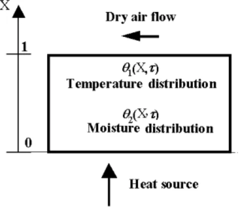
In Fig. 1, adapted from Mwithiga and Olwal (2005), it is represented the drying experiment setup considered in the present work. It was introduced the possibility of using a scale to weigh the samples and sensors to measure temperature in the sample, as well as inside the drying chamber. In order to obtain the variation of moisture content with time, from time to time samples are extracted from the drying chamber and weighed.
Figure 1. Drying experimental setup adapted from Mwithiga and Olwal (2005).
J. of the Braz. Soc. of Mech. Sci. & Eng. Copyright 2011 by ABCM October-December 2011, Vol. XXXIII, No. 4 / 401 Figure 2. Drying process schematic representation.
The mathematical formulation used in this work for the direct heat and mass transfer problem considered a constant properties model, which in the dimensionless form is given by (Mikhailov and Özisik, 1994):
( )
2 2 2 2 1 2 1 , X X X ∂ ∂ − ∂ ∂ = ∂∂ α θ β θ
τ τ
θ , 0<X<1, τ>0 (1)
( )
2 1 2 2 2 2 2 , X Lu Pn X Lu X ∂ ∂ − ∂ ∂ = ∂∂ θ θ
τ τ
θ , 0<X<1, τ>0 (2)
subject to the initial conditions, for 0≤X ≤1,
( ,0) 0
1 X =
θ (3)
( ,0) 0
2 X =
θ (4)
and to the boundary conditions, for
τ
>0,( )
0,1
Q X =− ∂ ∂θ τ
(5)
( )0,
2 PnQ
X =−
∂
∂θ τ (6)
( )1, ( )1, 1
1 + =
∂
∂θ τ θ τ
q
Bi
X
(
)
[
( )
]
0 , 1 1
1− − 2 =
− ε m θ τ
q KoLuBi
Bi
(7)
( )
+( )
=∂
∂θ 1,τ θ 1,τ
2 * 2
m
Bi
X
[
1( )1, 1]
*− θ τ −
q
m Pn Bi
Bi
(8)
where
Ko Lu Pn 1 ε
α= + (9)
Ko Lu
ε
β = (10)
( )
[
εPn Ko Lu]
Bi
Bi m
*
m= 1−1− (11)
and the dimensionless variables are defined as
(
) ( )
0 0 1 , , T T T t x T X s− − = τθ , temperature (12)
( )
( )
* 0 0 2 , , u u t x u u X − − = τθ , moisture potential (13)
l x
X= , spatial coordinate (14)
2 l at
=
τ , time (15)
a a
Lu= m, Luikov number (16)
* 0 0 u u T T Pn s − −
=δ , Possnov number (17)
0 * 0 T T u u c r Ko s− −
= , Kossovitch number (18)
k hl
Biq= , heat Biot (19)
m m m k l h
Bi = , mass Biot (20)
(
T T0)
k ql Q
s−
= , heat flux (21)
When the geometry, the initial and boundary conditions, and the medium properties are known, the system of equations (1)-(8) can be solved, yielding the temperature and moisture distribution in the media. In this work the finite difference method is used to solve such system.
Many previous works have studied the drying inverse problem using measurements of temperature and moisture potential at specific locations of the medium. But, to measure the moisture potential in a certain position is not an easy task. Therefore, in this work it is used the average quantity
( )
u( )xtdx l t u l x x∫
= = = 0 ,1 (22)
or
( )
X dXX X
∫
= = = 1 0 22τ θ ( ,τ)
θ (23)
Therefore, in order to obtain the average moisture measurements, u(t), one has just to weigh the sample at each time of observation.
Inverse Problem Formulation
The inverse problem considered is implicitly formulated as a finite dimensional optimization problem where one seeks to minimize the objective function of squared residues (Silva Neto and Soeiro, 2003).
[
G P G] [
WG P G]
F WFP T meas calc T meas calc
where Gmeas is the vector of measurements, Gcalc is the vector of calculated values, P is the vector of unknowns, W is the diagonal matrix whose elements are the inverse of the measurement variances, and the vector of residues F is given by
meas
calc P G
G
F= ( )− (24b)
The inverse problem solution is the vector *
P which minimizes
the norm given by Eq. (24a), i.e.
) ( min ) ( *
P P
P S
S =
(25)
Using temperature measurements, q1, acquired by sensors located inside the medium, and the average of the moisture potential, u, during the experiment, we try to estimate the vector of unknowns P. In the present work a combination of unknown variables was used: Lu (Luikov number), δ (thermogradient coefficient), r/c (relation between latent heat of evaporation and specific heat of the medium), h/k (relation between heat transfer coefficient and thermal conductivity), and hm/km (relation between
moisture transfer coefficient and mass conductivity).
Experiment Design
Much research effort has already been made in order to estimate the Possnov, Kossovitch, heat Biot and mass Biot numbers (Dantas et al., 2003; Huang and Yeh, 2002; Lugon and Silva Neto, 2004), and it was considered the possibility of optimizing the number and location of temperature sensors, experiment duration, etc. In this work instead, d, r/c, h/k and hm/km are estimated using an
“optimum” experiment (Dowding et al., 1999; Beck, 1988) designed for wood drying, and doing so it was considered the following process control parameters: heat flux, Q, the medium width, l, difference between the medium and the air temperatures,
0
T T
dT = s− , and difference between the moisture potential in the
medium and the air, *
0 u
u
du= − .
The sensitivity analysis plays a major role in several aspects related to the formulation and solution of an inverse problem. Such analysis may be performed with the study of the sensitivity coefficients. Here we use the modified, or scaled sensitivity coefficients
( ) ( ) p
j j j
N j
P X V P X P
SC , ∂ , , =1 ,2,L,
∂
= τ
τ
(26)
where V is the observable state variable (which can be measured), Pj
is a particular unknown of the problem, and Np is the total number
of unknowns.
There is no difference between the sensitivity coefficients for the two sets of variables, that is, the scaled sensitivity coefficients are exactly the same for both sets of unknowns
{
}
Tm q Bi
Bi Ko Pn
Lu, , , , ,ε and
{
Lu,δ
,r c,h k,hm km,ε
}
T,( ) ( ) ( τ) ( τ)
δ τ
δ τ
δ , , , X,
Pn SC Pn
X V Pn X V X
SC =
∂ ∂ = ∂ ∂
= (27)
( ,τ) ( ,τ) ( ,τ) (X,τ)
Ko SC Ko
X V Ko c r
X V c r X c r
SC =
∂ ∂ = ∂ ∂
= (28)
( ,τ) ( ,τ) ( ,τ) (X,τ)
Bi SC Bi
X V Bi k h
X V k h X k h SC
q
q =
∂ ∂ = ∂ ∂
= (29)
( ,τ) ( ,τ) ( ,τ) (X,τ)
Bi SC Bi
X V Bi k h
X V k h X k h SC
m m
m m m m m m
m
= ∂ ∂ = ∂ ∂ =
(30)
The reason for choosing the second set of unknowns to be estimated is based on the use of experiment design tools and interpretation. Consider the heat and mass Biot numbers for example. If one changes the medium width,
l
, both heat and mass Biot numbers change. The mathematical problem would be different, even though the material is still the same, because one is estimating two different heat and mass Biot numbers. In order to avoid this situation, it was decided to estimate the relation between heat transfer coefficient and thermal conductivity, h/k, and the relation between mass transfer coefficient and mass conductivity,hm/km, so that we could change the medium width and continue with
the same value for both variables to be estimated.
The same reasoning was used in the decision of estimating the thermogradient coefficient (
δ
) and the relation between latent heat of evaporation and specific heat of the medium (r/c), instead of the Possnov (Pn) and Kossovitch (Ko) numbers. Doing so, one is able to optimize the experiment considering the difference between the medium and the air temperatures, dT=Ts−T0, and the differencebetween the moisture potential between the medium and the air,
*
0 u
u
du= − , without affecting the values of the unknown parameters.
As a general guideline, the sensitivity of the state (observable) variable to the unknown parameter we want to estimate must be high enough to allow estimation within reasonable confidence bounds. Moreover, when two or more parameters are simultaneously estimated, their effects on the state variable must be independent (uncorrelated). Therefore, when represented graphically the sensitivity coefficients should not have the same shape. If they do it means that two or more different parameters affect the state variable in the same way, being difficult to distinguish their influences separately, which yields to poor estimations.
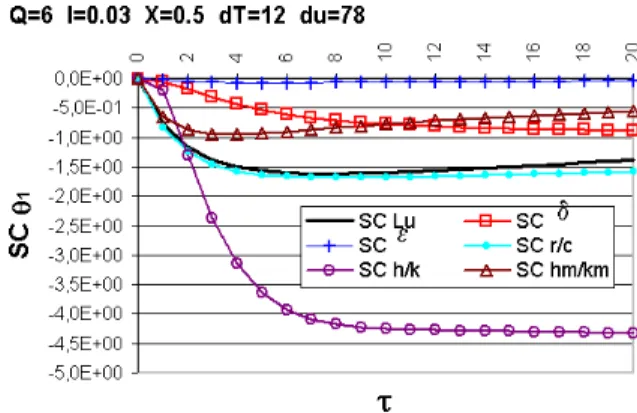
Since it was observed that the temperature sensor location did not influence significantly the sensitivity, we fixed its location at
5 . 0 =
X .
In Figs. 3 and 4, it is represented the sensitivity coefficients for temperature and moisture potential for a specific case in which are considered the following geometric and process parameters: l = 0.03 m, Q = 6.0, dT = 12 K and du = 78 °M. Since the sensitivity to the parameter ε is too low for both the temperature and moisture measurements, the estimation of this parameter is not considered in this work.
J. of the Braz. Soc. of Mech. Sci. & Eng. Copyright 2011 by ABCM October-December 2011, Vol. XXXIII, No. 4 / 403 Figure 4. Sensitivity coefficients for moisture potential.
Another important tool used in this work to design the experiment consists on the study of the matrix
=
m P N m
m
m P N
m P N
V P V
P V
P
V P V
P V
P
V P V
P V
P
SC
SC
SC
SC
SC
SC
SC
SC
SC
...
...
...
...
...
...
...
2 1
2 2 2
1
1 2 1
1
Y
(31)where
V
i is a particular measurement of temperature or moisturepotential and
m
is the total number of measurements. With1
θ
m
data points for the temperature and
2
θ
m for the moisture potential,
one has
2
1 θ
θ m m
m= + .
Maximizing the determinant of the matrix YT Y results in higher
sensitivity and uncorrelation (Beck, 1988).
In Fig. 5 it is represented the variation of the value of the matrix
YT Y determinant as a function of the temperature differences and
moisture potential differences between the medium and the dry air flowing over it. In order to achieve greater sensitivities, while the temperature difference has to be the lowest, the moisture potential difference has to be the highest possible. The solid square represents the chosen designed experiment, considering the existence of practical difficulties that may limit our freedom of choice.
Figure 5. Matrix YTY determinant as a function of temperature ( dT) and moisture potential (du) differences.
In Fig. 6 it is represented the values of the determinant of matrix
YT Y for different values of the heat flux Q and medium thickness l.
For practical reasons it was chosen to limit the sample temperature to 130ᴼC. In Fig. 6 when the sample temperature exceeds the limit of 130ᴼC it is used a dashed-line representation. The solid square represents the chosen designed experiment.
Figure 6. YT Y matrix determinant for different values of the heat flux Q and
medium thickness l.
Considering the previous analysis of the sensitivity graphs and of the matrix YT Y determinant, it was designed the experiment
whose geometric and process parameters are shown in Table 1. Since the average moisture potential,
θ
2 or u, is more difficult to measure than temperature,θ
1, the measurement interval for the average moisture potential, ∆τ
u, was considered larger than theinterval for the temperature
1
θ
τ
∆
.Table 1. Reference values for the designed experiment. ττττ0 and ττττf represent
the initial and final sampling times, respectively.
Geometric or process parameter
Values
0
T
T
dT
=
s−
12 K0
T
297 Ks
T 309 K
*
0
u
u
du
=
−
78 oM0
u 86 oM
*
u 8 oM
ε
0.2Q 6.0
l
0.03 m0
τ
0f
τ
201
θ
τ
∆
0.21
θ
m
1002
θ
τ
∆
12
θ
Inverse Problem Solution
In this work we used one Artificial Neural Network (ANN) to generate the initial guess for the Levenberg-Marquardt (LM) method, another ANN to approximate the gradient needed by LM, and, finally, the global minimum was searched using the SA for the minimization of the objective function given by Eq. (24a).
The Levenberg-Marquardt method (LM)
The Levenberg-Marquardt method is a deterministic local optimization method based on the gradient of the objective function. In order to minimize the functional
S
we first write0 )
( =
= F WF
P P
T
d d d
dS
→
JTWF=0 (32)where J is the Jacobian matrix, whose elements are
s p
ps P
J ====∂∂∂∂θ1 ∂∂∂∂ , for p=1,2,...mθ1
, Jps=∂θ2p ∂Ps, for
2 1 1 1,..., θ θ
θ m m
m
p= + + and s=1,2,...Np. Observe that the
elements of the Jacobian matrix are related to the scaled sensitivity coefficients presented before.
Using a Taylor’s expansion and keeping only the terms up to the first order:
(
P P) ( )
FP J PF +∆ ≅ + ∆ (33)
and introducing the above expansion in Eq. (32) results
( )
P WF J P WJJT ∆ =− T (34)
In the Levenberg-Marquardt method it is added to the diagonal of matrix JTWJ a damping factor λ to help to achieve convergence.
The value of λ is varied along the iterative process with λ→ 0 when convergence is achieved.
Equation (34) is then written in a more convenient form to be used in the iterative procedure:
( )
[
nT n n]
( )
nT( )
nn J WJ I J WFP
P =− + −1
∆ λ (35)
where I is the identity matrix, and
n
is the iteration counter. The iterative procedure starts with an estimate for the unknown parameters,P
0, being new estimates obtained with n n nP P P+1= +∆ , while the corrections n
P
∆ are calculated with Eq. (35). This iterative procedure is continued until a convergence criterion such as
P n
k n
k P k N
P < , =1,2,...,
∆ ε (36)
is satisfied, where
ε
is a small number, e.g. 10-5.The elements of the Jacobian matrix as well as the right hand side term of Eq. (34) are updated at each iteration, using the solution of the direct problem with the estimates for the unknowns obtained in the previous iteration.
The Artificial Neural Network (ANN)
The multi-layer perceptron, MLP, (Haykin, 1999) is a collection of connected processing elements called nodes or neurons, arranged in layers (see Fig. 7). Signals pass into the input layer nodes,
emerge from the output layer. Each node i is connected to each node j in its preceding layer through a connection of weight wij, and similarly to nodes in the following layer.
A weighted sum is performed at node i of all the signals xj from
the preceding layer, yielding the excitation of the node; this is then passed through a nonlinear activation function, f, to emerge as the output of the node i to the next layer
=
∑
j j ij i f w x
y
(37)
Various choices for the function f are possible. In this work the hyperbolic tangent function f(x)=tanh(x) is used.
Figure 7. Multi-layer perceptron network.
The first stage of using an ANN to model an input-output system is to establish the appropriate values for the connection weights wij. This is the “training” or learning phase. Training is accomplished using a set of network inputs for which the desired outputs are known. These are the so called patterns, which are used in the training stage of the ANN. At each training step, a set of inputs are passed forward through the network yielding trial outputs which are then compared to the desired outputs. If the comparison error is considered small enough, the weights are not adjusted. Otherwise, the error is passed backwards through the net and a training algorithm uses the error to adjust the connection weights. This is the back-propagation algorithm used in the present work.
First of all, the training patterns are generated using the direct problem solution. For that purpose ten intervals were taken for each parameter, ranging from 50% up to 150% of the exact parameter values. The ANN used to solve the direct problem was trained to calculate the temperature and average moisture potential values, being informed in the input layer the following quantities: Lu, d, r/c, h/k, hm/km, τ. This ANN was also used to approximate the
derivatives necessary to calculate the elements of the Jacobian matrix for LM, with respect to each parameter, using a central difference approximation.
The other ANN, dedicated to solve the inverse problem, used a set of five values of temperature measurements,
1
θ
m , and five values
of average moisture potential,
2
θ
m , to estimate simultaneously the
parameters Lu, d, r/c, h/k, hm/km. The patterns used in the training
J. of the Braz. Soc. of Mech. Sci. & Eng. Copyright 2011 by ABCM October-December 2011, Vol. XXXIII, No. 4 / 405
parameters. The number of patterns generated was 3,125 for the inverse problem, and 31,250 for the direct problem.
The training of each ANN consisted of 2,000 epochs varying randomly the order of patterns presentation.
Once the comparison error is reduced to an acceptable level over the whole training set, the training phase ends and the network is established. After that, the parameters of a model (output) may then be determined using the real experimental data, which are the inputs of the established neural network developed for the problem solution. This is the generalization stage in the use of the ANN.
The Simulated Annealing method (SA)
Based on statistical mechanics reasoning, applied to a solidification problem, Metropolis et al. (1953) introduced a simple algorithm that can be used to accomplish an efficient simulation of a system of atoms in equilibrium at a given temperature. In each step of the algorithm a small random displacement of an atom is performed and the variation of the energy ∆E is calculated. If ∆E<0 the displacement is accepted, and the configuration with the displaced atom is used as the starting point for the next step. In the case of ∆E>0, the new configuration may be accepted according to the Boltzmann probability:
( )
E(
E k T)
P∆ =exp−∆ / B (38)
A uniformly distributed random number p is generated in the interval [0,1] and compared with P(∆E). Metropolis criterion establishes that the new configuration is accepted if p<P(∆E); otherwise, it is rejected and the previous configuration is used again as a starting point.
Kirkpatrick et al. (1983) developed an optimization algorithm inspired in the cooling problem described above using the Metropolis criterion, the so called Simulated Annealing (SA) method. Using the objective function S(P), given by Eq. (24a), in place of energy, and defining configurations by a set of variables
{ }
Pi ,i=1,2,...,Np, where Np represents the number of unknowns wewant to estimate, the Metropolis procedure generates a collection of configurations of a given optimization problem at some temperature T. This temperature is simply a control parameter. The simulated annealing process consists of first “melting” the system being optimized at a high “temperature”, then lowering the “temperature” until the system “freezes” and no further change occurs.
The main control parameters of the algorithm implemented (“cooling procedure”) are the initial “temperature”, T0, the cooling rate, rt, number of steps performed through all elements of vector P, Ns, number of times the procedure is repeated before the
“temperature” is reduced, Nt, and the number of points of minimum
(one for each temperature) that are compared and used as the stopping criterion if they all agree within a tolerance ε, Nε.
Combination of ANN, LM and SA optimizers
After the training stage, an ANN is able to quickly obtain an inverse problem solution. This solution is then used as an initial guess for the LM.
Due to the complexity of the design space, if convergence is achieved with a gradient based method it may in fact correspond to a local minimum. Therefore, global optimization methods are required in order to reach the global minimum, or at least its vicinity. The main disadvantage of these methods is that the number of function evaluations is high, becoming sometimes prohibitive from the computational point of view (Soeiro et al., 2004a,b).
Trying to keep the best features of each method, we have combined the ANN developed for the solution of the inverse problem, the LM and the SA methods. First we used the ANN, obtaining quickly an initial guess for the LM. We then ran the LM, reaching within a few iterations a point of minimum. After that we ran the SA. If the same solution was reached, it was likely that a global minimum was found, and the iterative procedure was interrupted. If a different solution was obtained, it meant that the previous one was a local minimum. In that case we could run again the LM and SA until the global minimum was reached.
The canonical LM depends on the calculation of the gradient, which in many cases must be approximated by finite differences. In practice it means that the direct problem has to be solved many times. As previously described, in this work an ANN was trained to solve the direct problem and then it was used to approximate the gradient in the first steps of the LM. After this initial stage a refinement in the solution was implemented, with the use of finite differences for the calculation of the gradient.
Results
An experiment was designed to perform the simultaneous estimation of Lu, δ, r/c, h/k, hm/km. In order to study the proposed
method, since real experiment data were not available, we generated synthetic data using
i exact calc
measi 1 i(P ) 1r
1 θ σθ
θ = r +
,
1
,..., 2 , 1 mθ i=
(39a)
i exact calc
measi 2 i(P ) 2r
2
θ
σ
θθ
= r +,
2
,..., 2 ,
1 mθ
i=
(39b)
where ri are random numbers in the range [-1,1], m and θ1
2
θ m
represent the total number of temperature and moisture potential experimental data, and σθ1 and σθ2 emulates the standard deviation
of measurement errors. It was used 0.03
1=
θ
σ considering 100 temperature measurements (∆τ=0.2), resulting in a maximum error of 2%, and 0.001
2=
θ
σ considering 20 moisture measurements (∆τ=1.0), resulting in a maximum error of 4%.
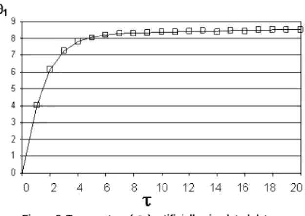
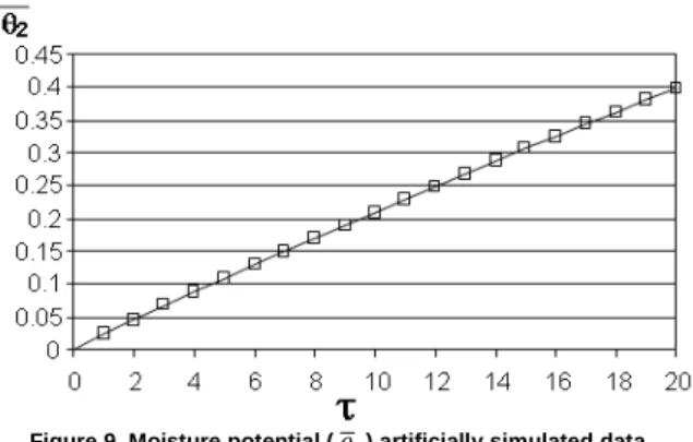
In Figs. 8 and 9, it is shown the temperature (θ1) and the moisture potential (θ2) measurements, respectively, represented by squares, and the solid lines correspond to the direct problem solution using the parameters estimated with the inverse problem solution. In order to give a clearer representation, only 20 temperature (θ1) measurements were represented.
Figure 8. Temperature (
1
Figure 9. Moisture potential ( 2
θ ) artificially simulated data.
The results obtained using the LM 1 (gradient approximated by finite differences), LM 2 (gradient approximated by ANN), ANN, SA and hybrid combinations, for different levels of noise represented by different values for the standard deviation of measurements errors in temperature and average moisture potential,
1
θ
σ and
2
θ
σ , are shown in Table 2. In parenthesis are shown the percentage errors between the estimates and the exact values of the unknowns.
One observes that when there is no noise, that is, the standard deviation of measurements errors is null, the LM method was able to estimate all variables very quickly (test cases 1 and 2). When noise is introduced, the LM is retained by local minima (test cases 3 and 4). The ANN alone did not reach a good solution, but quickly got close to it (test case 5). The ANN solution was used as a first guess for the LM method with good performance in test cases 6 and 7. The SA alone reached a reasonable solution (test case 8), but it required a high computational time. Finally, the combination of all methods was able to reach a good solution (test case 9), without being retained by local minima, and without taking too much time, i.e. six times less than SA. The time shown in the sixth column of Table 2 corresponds to the CPU time on a Pentium IV 2.8 GHz processor.
Conclusions
The direct problem of simultaneous heat and mass transfer in porous media, modeled with Luikov equations, can be solved using the finite difference method, yielding the temperature and moisture distribution in the media, when the geometry, the initial and boundary conditions as well as the medium properties are known.
Inverse problem techniques can be useful to estimate the medium properties when they are not known. After the use of an experiment design technique, the hybrid combination ANN-LM-SA resulted in good estimates for the drying inverse problem using artificially generated data.
The design of experiment technique is of great importance for the success of the estimation. While previous works studied the estimation of Lu, Pn, Ko, Biq and Bim, in this work it was considered
Lu, δ, r/c, h/k and hm/km. The main advantage is to be able to design
an “optimum” experiment using different medium width, l, porous medium and air temperature difference, Ts – T0, and porous medium and air moisture potential difference, *
0 u
u − .
The combination of deterministic (LM) and stochastic (ANN and SA) methods achieved good results, reducing the time needed and not being retained by local minima. The use of ANN to obtain the derivatives in the first steps of the LM method reduced the time required for the solution of the inverse problem.
The next step of this research is to study the impact of larger measurement deviation and to use real experiment data to estimate medium properties for industrial cases of interest.
Acknowledgements
The authors acknowledge the financial support provided by CNPq – Conselho Nacional de Desenvolvimento Científico e Tecnológico, and FAPERJ – Fundação Carlos Chagas Filho de Amparo à Pesquisa do Estado do Rio de Janeiro.
References
Beck, J.V., 1988, “Combined Parameter and Function Estimation in Heat Transfer with Application to Contact Conductance”, J. Heat Transfer, Vol. 110, pp. 1046-1058.
Bialobrzewski, I, 2007, “Determination of the Mass Transfer Coefficient During Hot-Air-Drying Celery Root”, J. of Food Engineering, Vol. 78, pp. 1388-1396.
Dantas, L.B., Orlande, H.R.B. and Cotta, R.M, 2003, “An Inverse Problem of Parameter Estimation for Heat and Mass Transfer in Capillary Porous Media”, Int. J. Heat Mass Transfer, Vol. 46, pp. 1587-1598.
Dowding, K.J., Blackwell, B.F. and Cochran, R.J., 1999, “Applications of Sensitivity Coefficients for Heat Conduction Problems”, Numerical Heat
Transfer, Part B, Vol. 36, pp. 33-55.
Haykin, S., 1999, “Neural Networks – A Comprehensive Foundation”, Prentice Hall.
Huang, C.H. and Yeh, C.Y., 2002, “An Inverse Problem in Simultaneous Estimating the Biot Number of Heat and Moisture Transfer for a Porous Material”, Int. J. Heat Mass Transfer, Vol. 45, pp. 4643-4653.
Kanevce, L.P. Kanevce, G.H. and Dulikravich, G.S., 2002a, “Estimation of Drying Food Thermophysical Properties by Using Temperature Measurements”, 4th International Conference on Inverse Problems in
Engineering, Vol. II, pp. 299-306, Angra dos Reis, Brazil.
Kanevce, G.H. Kanavce, L.P. Dulikravich, G.S. and Orlande, H.R.B., 2002b, “Estimation of Thermophysical Properties of Moist Materials Under Different Drying Conditions”, 4th International Conference on Inverse
Problems in Engineering, Vol. II, pp. 331-338, Angra dos Reis, Brazil. Kirkpatrick, S., Gellat, Jr., C.D. and Vecchi, M.P., 1983, “Optimization by Simulated Annealing”, Science, Vol. 220, pp. 671-680.
Lugon Jr., J. and Silva Neto, A.J., 2004, “Deterministic, Stochastic and Hybrid Solutions for Inverse Problems in Simultaneous Heat and Mass Transfer in Porous Media”, Proc. 13th Inverse Problems in Engineering
Seminar, pp. 99-106, Cincinatti, USA.
Luikov, A.V. and Mikhailov, Y.A, 1965, “Theory of Energy and Mass Transfer”, Pergamon Press, Oxford, England.
Metropolis, N., Rosenbluth, A.W., Rosenbluth, M.N., Teller, A.H. and Teller, E., 1953, “Equation of State Calculations by Fast Computing Machines”, J. Chem. Physics, Vol. 21, pp. 1087-1092.
Mikhailov, M.D. and Özisik, M.N., 1994, “Unified Analysis and Solutions of Heat and Mass Diffusion”, Dover Publications, Inc.
Mwithiga, G., and Olwal, J.O., 2005, “The Drying Kinetics of Kale (Brassica Oleracea) in a Convective Hot Air Dryer”, J. of Food Engineering, Vol. 71, No. 4, pp. 373-378.
Pavón-Melendez, G., Hernández, J.A., Salgado, M.A. and Garcia, M.A., 2002, “Dimensionless Analysis of the Simultaneous Heat and Mass Transfer in Food Drying”, J. of Food Engineering, Vol. 51, pp. 347-353.
Pedreño-Molina, J.L., Monzó-Cabrera, J. and Sánchez-Hernández, D., 2005a, “A New Predictive Neural Architeture for Solving Temperature Inverse Problems in Microwave-assisted Drying Process”, Neurocomputing, Vol. 64, pp. 521-528.
Pedreño-Molina, J.L., Monzó-Cabrera, J., Toledo-Moreo, A. and Sánchez-Hernández, D., 2005b, “A Novel Predictive Architeture for Microwave-assisted Drying Process Based on Neural Networks”, Int. Comm.
in Heat and Mass Transfer, Vol. 32, pp. 1026-1033.
Pedreño-Molina, J.L., Monzó-Cabrera, J., Toledo-Moreo, A. and Sánchez-Hernández, D., 2005c, “Estimation of Microwave-Assisted Drying Parameters Using Adaptative Optimization Techniques”, Int. Comm. in Heat
and Mass Transfer, Vol. 32, pp. 323-331.
Silva Neto, A.J. and Soeiro, F.J.C.P., 2003, “Solution of Implicitly Formulated Inverse Heat Transfer Problems with Hybrid Methods”, Mini-Symposium Inverse Problems from Thermal/Fluids and Solid Mechanics Applications – 2nd MIT Conference on Computational Fluid and Solid
Mechanics, Cambridge, USA.
J. of the Braz. Soc. of Mech. Sci. & Eng. Copyright 2011 by ABCM October-December 2011, Vol. XXXIII, No. 4 / 407
and Hybrid Methods”, Proc. 13th Inverse Problems in Engineering
Seminar, pp. 163-169, Cincinnati, USA.
Soeiro, F.J.C.P., Soares, P.O., Campos Velho, H.F. and Silva Neto, A.J., 2004b, “Using Neural Networks to Obtain Initial Estimates for the Solution
of Inverse Heat Transfer Problems”, Proc. Inverse Problems, Design and Optimization Symposium, Vol. I, pp. 358-363, Rio de Janeiro, Brazil.
Whitaker S., 1977, “Simultaneous Heat, Mass and Momentum Transfer in Porous Media: A Theory of Drying”, Advances in Heat and Mass
Transfer, Vol. 13, pp. 110-203.
Table 2. Results obtained using LM 1, LM 2, ANN, and hybrid combinations. σθ1 = 0.03 corresponds to a 2% noise level in temperature data. 2
θ
σ = 0.001 corresponds to a 4% noise level in moisture potential data.
C
as
e
Method
1
θ
σ
2
θ
σ
S
Eq. (24a)
Time
(s) Information Lu δ r/c h/k hm/km
- - - Exact values 0.0080 2.0 10.83 34.0 114.0
1 LM 1
(grad. FDM) 0 0 0 15
Initial guess 0.0040 1.50 8.00 20.0 80.0
Result
Z
LMFDM 0.0080(0%)
2.00 (0%)
10.83 (0%)
34.0 (0%)
114.0 (0 %)
2 LM 2
(grad. ANN) 0 0 0 10
Initial guess 0.0040 1.50 8.00 25.0 80.0
Result ANN
LM
Z
0.0080 (0%) (0%) 2.00 10.83 (0%) 34.0 (0%) 114.0 (0%)3 LM 1
(grad. FDM) 0.03 0.001 977 15
Initial guess 0.0040 1.50 8.00 20.0 80.0
Result FDM
LM
Z
0.0076(5%)
2.09 (4.5%)
10.76 (0.6%)
34.1 (0.3%)
121.2 (6.3%)
4 LM 2
(grad. ANN) 0.03 0.001 897 11
Initial guess 0.0040 1.50 8.00 20.0 80.0
Result
Z
LMANN 0.0093(16%)
1.71 (14%)
10.73 (0.9%)
34.1 (0.3%)
95.7 (16%)
5 ANN (without
initial guess) 0.03 0.001 3190 1 Result
Z
ANN0.0083 (3.8%)
2.10 (5%)
10.04 (7.3%)
35.0 (2.9%)
117.1 (2.7%)
6 LM 1
(grad. FDM) 0.03 0.001 974 16
Initial guess
Z
ANN 0.0083 2.10 10.04 35.0 117.1Result FDM
LM
Z
0.0083(3.8%)
1.92 (4%)
10.75 (0.7%)
34.1 (0.3%)
110.0 (3.5%)
7 LM 2
(grad. ANN) 0.03 0.001 903 11
Initial guess
Z
ANN 0.0083 2.10 10.04 35.0 117.1Result
Z
LMANN0.0082 (2.5%)
1.79 (10.5%)
9.89 (8.7%)
35.1 (3.2%)
114.5 (0.4%)
8
SA (SA 20,000
function evaluations)1
0.03 0.001 856 300
Initial guess 0.0040 1.50 8.00 25.0 80.0
Result
Z
SA 0.0094 (17.5%)1.58 (21%)
9.96 (8%)
35.0 (2.9%)
98.2 (14%)
9
ANN-LM 2-SA (SA 2,000
function evaluations)1
0.03 0.001 760 47
Initial guess
Z
ANN 0.0083 2.10 10.04 35.0 117.1Result
Z
LMANN 0.0082(2.5%)
1.79 (19.5%)
9.89 (8.7%)
35.1 (3.2%)
114.5 (0.4%)
Result
Z
SA 0.0079 (1.3%) (0.5%)2.01 (1.5%)11.00 (0.3%)33.9 (0.2%)113.8Result
Z
LMANN 0.0080(0%)
2.05 (2.5%)
10.93 (0.9%)
33.8 (0.6%)