Effects of long-range aerosol transport on the microphysical properties of low-level liquid clouds in the Arctic

(1)

ACPD

15, 31823–31866, 2015

Effects of pollution on liquid clouds in

the Arctic

Q. Coopman et al.

Title Page

Abstract Introduction

Conclusions References

Tables Figures

◭ ◮

Back Close

Full Screen / Esc

Printer-friendly Version

Interactive Discussion

Discussion

P

a

per

|

Discussion

P

a

per

|

Discussion

P

a

per

|

Discussion

P

a

per

|

Atmos. Chem. Phys. Discuss., 15, 31823–31866, 2015 www.atmos-chem-phys-discuss.net/15/31823/2015/ doi:10.5194/acpd-15-31823-2015

This discussion paper is/has been under review for the journal Atmospheric Chemistry and Physics (ACP). Please refer to the corresponding final paper in ACP if available.

E

_ff

ects of long-range aerosol transport on

the microphysical properties of low-level

liquid clouds in the Arctic

Q. Coopman1,2, T. J. Garrett1, J. Riedi2, S. Eckhardt3, and A. Stohl3

1

Department of Atmospheric Sciences, University of Utah, Salt Lake City, UT, USA

2

Laboratoire d’Optique Atmosphérique, Université de Lille/CNRS, France

3

Norwegian Institute for Air Research, Keller, Norway

Received: 1 October 2015 – Accepted: 23 October 2015 – Published: 12 November 2015 Correspondence to: Q. Coopman (quentin.coopman@ed.univ-lille1.fr)

(2)

ACPD

15, 31823–31866, 2015

the Arctic

Q. Coopman et al.

Title Page

Tables Figures

◭ ◮

Back Close

Full Screen / Esc

Discussion

P

a

per

|

Discussion

P

a

per

|

Discussion

P

a

per

|

Discussion

P

a

per

|

Abstract

The properties of clouds in the Arctic can be altered by long-range aerosol transport to the region. The goal of this study is to use satellite, tracer transport model, and meteo-rological data sets to determine the eff_{ects of pollution on cloud microphysics due only}

to pollution itself and not to the meteorological state. Here, A-Train, POLDER-3 and

5

MODIS satellite instruments are used to retrieve low-level liquid cloud microphysical properties over the Arctic between 2008 and 2010. Cloud retrievals are co-located with simulated pollution represented by carbon-monoxide concentrations from the FLEX-PART tracer transport model. The sensitivity of clouds to pollution plumes – including aerosols – is constrained for cloud liquid water path, temperature, altitude, specific

10

humidity, and lower tropospheric stability (LTS). We define an Indirect Eff_{ect (IE)}

pa-rameter from the ratio of relative changes in cloud microphysical properties to relative variations in pollution concentrations. Retrievals indicate that, depending on the me-teorological regime, IE parameters range between 0 and 0.34 for the cloud droplet eff_{ective radius, and between}₋_{0.10 and 0.35 for the optical depth, with average values} 15

of 0.12±0.02 and 0.15±0.02 respectively. The IE parameter increases with increasing specific humidity and LTS. Further, the results suggest that for a given set of meteo-rological conditions, the liquid water path of arctic clouds does not respond strongly to pollution. Or, not constraining suffi_{ciently for meteorology may lead to artifacts that}

ex-aggerate the magnitude of the aerosol indirect eff_{ect. The converse is that the response} 20

of arctic clouds to pollution does depend on the meteorologic state. Finally, we find that IE values are highest when pollution concentrations are low, and that they depend on the source of pollution.

1 Introduction

Due to growing concentrations of green house gases, including atmospheric carbon

25

(3)

ACPD

15, 31823–31866, 2015

the Arctic

Q. Coopman et al.

Title Page

Tables Figures

◭ ◮

Back Close

Full Screen / Esc

Discussion

P

a

per

|

Discussion

P

a

per

|

Discussion

P

a

per

|

Discussion

P

a

per

|

global average due to feedback processes (Serreze and Francis, 2006; Serreze et al., 2009; Richter-Menge and Jeff_{ries, 2011), a trend that is anticipated to continue through}

this century (Yoshimori et al., 2013; Overland and Wang, 2013). Further, the Arctic is not pristine, even if it is remote from industrialized areas and major aerosol sources. Mid-latitude aerosols can be transported to northern latitudes in relatively high

concen-5

trations due to low precipitation and strong temperature inversions that inhibit vertical mixing (Sirois and Barrie, 1999; Law and Stohl, 2007; Quinn et al., 2007; Law et al., 2014). From spring to summer, the atmosphere becomes cleaner due to an increase in wet-scavenging (Garrett et al., 2010). The origins of arctic haze tend to be pollution from Eurasia (Shaw, 1995; Stohl, 2006; Shindell et al., 2008; Ancellet et al., 2014), and

10

boreal forest fires in North America, Eastern Europe and Siberia (Stohl, 2006; Stohl et al., 2007).

Such aerosols have the potential to alter cloud properties in the Arctic (Garrett and Zhao, 2006; Lance et al., 2011). On one hand, thin low-level clouds with more numer-ous smaller droplets can radiate more long wave radiation thereby warming the surface

15

(Garrett et al., 2002, 2004; Garrett and Zhao, 2006). On the other, polluted clouds can reflect more sunlight, leading to a cooling eff_{ect (Lubin and Vogelmann, 2007). Zhao}

and Garrett (2015) found that seasonal changes in surface radiation associated with haze pollution ranges from +_{12.2 W m}−2 _{in February to} ₋_{11.8 W m}−2 _{in August.}

An-nually averaged, the long-wave warming and shortwave cooling nearly compensate,

20

although the seasonal timing of the forcings may have implications for rates of sea ice melt (Belchansky et al., 2004; Markus et al., 2009).

The Influence of aerosols on cloud microphysical properties is often quantified us-ing an Indirect Eff_{ect (IE) parameter, expressible as the ratio of relative changes in}

cloud microphysical properties to variations in pollution concentrations, most typically

25

aerosols (Feingold et al., 2001; Feingold; 2003b). Garrett et al. (2004) used ground-based measurements of the cloud droplet eff_{ective radius and dried aerosol light}

scat-tering at Barrow (Alaska) to retrieve an indirect eff_{ect value for the cloud droplet}

(4)

ACPD

15, 31823–31866, 2015

the Arctic

Q. Coopman et al.

Title Page

Tables Figures

◭ ◮

Back Close

Full Screen / Esc

Discussion

P

a

per

|

Discussion

P

a

per

|

Discussion

P

a

per

|

Discussion

P

a

per

|

for cloud droplet eff_{ective radius range from 0.02 to 0.20 for mid-latitude continental}

clouds (Nakajima et al., 2001; Feingold, 2003a; Lohmann and Feichter, 2005; Myhre et al., 2007) and from 0.03 to 0.15 for mid-latitude oceanic clouds (Bréon et al., 2002; Sekiguchi, 2003; Kaufman et al., 2005; Myhre et al., 2007; Costantino and Bréon, 2013; Wang et al., 2014). Satellite instruments have the advantage of providing data

5

over large spatial scales, however satellite retrievals of aerosol concentrations are nor-mally obtained from air columns close to the analyzed cloud. The assumption is made of a horizontally homogeneous plume both within and without the cloud (Nakajima et al., 2001; Feingold et al., 2001; Sekiguchi, 2003). For large-scale cloud studies, this method potentially introduces bias since it is not obvious that pollution should be

10

uniform for diff_{erent meteorological regimes.}

Co-locating satellite cloud retrievals with passive pollution tracer output from a chem-ical transport model off_{ers an alternative approach for assessing the e}ff_{ect of pollution}

on clouds. In this way, cloud microphysical properties and pollution concentrations can be estimated at the same time, location, and meteorological regime (Schwartz et al.,

15

2002; Kawamoto et al., 2006; Avey et al., 2007). Active tracers experience both sources and sinks, for example through wet scavenging, dry deposition, and chemical reactions. Passive pollution tracers, on the other hand, are determined only by their source and subsequent dilution. Most importantly, passive tracers are decoupled from clouds and are unaff_{ected by wet scavenging. What can be expressed is the orthogonal sensitivity} 20

of clouds to pollution in a manner that accounts for the possibility of aerosol removal. If aerosols are scavenged during long-range transport, for example, then the cloud sen-sitivity to pollution is low even if the sensen-sitivity to aerosols remains high. An example of a passive tracer is carbon monoxide (CO), which is a combustion by-product and correlates with the anthropogenic Cloud Condensation Nuclei (CCN) close to pollution

25

sources (Longley et al., 2005).

(5)

Cer-ACPD

15, 31823–31866, 2015

the Arctic

Q. Coopman et al.

Title Page

Tables Figures

◭ ◮

Back Close

Full Screen / Esc

Discussion

P

a

per

|

Discussion

P

a

per

|

Discussion

P

a

per

|

Discussion

P

a

per

|

mak, 2015). For example, a reduced stability of the environmental temperature profile can allow for enhanced cloud droplet growth through increasing convection (Klein and Hartmann, 1993). This would be expected to lead to greater mixing of the aerosols with the cloudy air and greater aerosol impacts on cloud microphysical properties (Chen et al., 2014; Andersen and Cermak, 2015). Also, in the Arctic during the winter,

pollu-5

tion plumes from Asia are often associated with higher values of potential temperature than pollution plumes from Europe (Stohl, 2006). Thus, the observed impact of pollution plumes on clouds may be correlated with a particular meteorological regime.

Using the approach of co-locating a passive tracer from a tracer transport model and satellite observations, Tietze et al. (2011) presented an analysis of IE over the

10

Arctic from March to July 2008. Anthropogenic and biomass burning pollution was rep-resented with a CO passive tracer in the FLEXPART (FLEXible PARTicle dispersion model) tracer model (Stohl et al., 2005) and was co-located with POLDER-3 (Polar-ization and Directionality of the Earth’s Reflectance) and MODIS (Moderate Resolution Imaging Spectroradiometer) observations. Tietze et al. (2011) showed that the

sensitiv-15

ity of liquid cloud eff_{ective radius (r}_e_{) and optical depth (τ) to pollution has a maximum}

around the freezing point, and that the sensitivity decreases for both higher and lower temperatures. The optical depth was generally up to four times more sensitive than the eff_{ective radius. Their results also suggested that biomass burning pollution has}

a smaller yet significant impact on liquid cloud microphysical properties than

anthro-20

pogenic pollution, and that the IE parameters depend on altitude, LWP, and tempera-ture.

Our study extends the Tietze et al. (2011) research by adding two years of data, 2009 and 2010, and by constraining assessment of the IE parameter for lower tropospheric stability (LTS) and atmospheric specific humidity. Our results highlight the importance

25

(6)

ACPD

15, 31823–31866, 2015

the Arctic

Q. Coopman et al.

Title Page

Tables Figures

◭ ◮

Back Close

Full Screen / Esc

Discussion

P

a

per

|

Discussion

P

a

per

|

Discussion

P

a

per

|

Discussion

P

a

per

|

2 Data

The analyses in this study are based on a co-location of satellite retrievals of cloud properties, tracer transport model simulations of pollution locations and concentrations, and reanalysis data sets for meteorological fields.

2.1 Satellite cloud property retrievals 5

In this study we used two instruments, both part of the A-train mission (Stephens et al., 2002). The MODIS instrument on board the Aqua satellite measures 36 diff_erent

spec-tral bands from 400 nm to 14 400 nm in wavelength. For retrievals of the eff_{ective radius,}

optical depth, and cloud top temperature we use Collection 5 Level-2 products (Plat-nick et al., 2003; King and Plat(Plat-nick, 2006). Cloud top temperature is derived from the

10

11 µm infrared band. Cloud droplet eff_{ective radius (r}_e_{) and optical depth (τ) are}

re-trieved from simultaneous cloud-reflectance measurements in three water absorbing bands (1.6, 2.1, 3.7 µm) and three non-absorbing bands (0.65, 0.86, 1.2 µm) (Platnick et al., 2003). The pixel resolution of the retrievals at nadir is 1 km for cloud microphysics and 5 km for cloud top temperature.

15

The POLDER-3 camera on the PARASOL satellite platform (Polarization & Anisotropy of Reflectances for Atmospheric Sciences coupled with Observations from a Lidar) captures a wide field of view through spectral, directional, and polarized mea-surements of reflected sunlight (Fougnie et al., 2007). Multidirectional observations al-low for a pixel to be observed from up to sixteen diff_{erent view angles. The instrument} 20

measures radiance in 9 spectral channels between 443 and 1020 nm, including three polarized channels at 490, 670 and 865 nm. POLDER-3 cloud microphysical properties retrievals have a 36 km2spatial resolution. Cloud top pressure is derived from the cloud oxygen pressure (Bréon and Colzy, 1999). Cloud top pressure retrieved by POLDER-3 appears to be a better proxy for low-level cloud height than MODIS cloud top pressure

25

(7)

ACPD

15, 31823–31866, 2015

the Arctic

Q. Coopman et al.

Title Page

Tables Figures

◭ ◮

Back Close

Full Screen / Esc

Discussion

P

a

per

|

Discussion

P

a

per

|

Discussion

P

a

per

|

Discussion

P

a

per

|

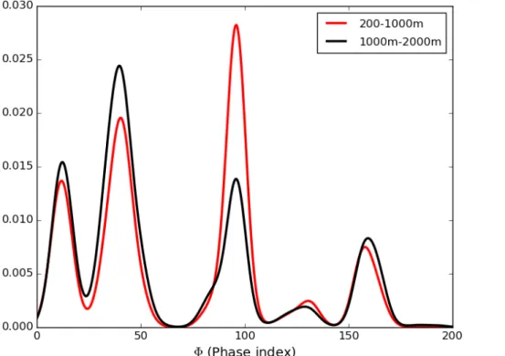
To determine the cloud thermodynamic phase we use a combination of MODIS and POLDER-3 measurements. The algorithm takes advantage of multi-angle polarization data, shortwave, thermal infrared, and visible measurements to retrieve a thermody-namic phase indexΦ _{between 0 for liquid clouds and 200 for ice clouds with varying}

degrees of confidence (Riedi et al., 2010). Figure 1 shows the distribution of the

ther-5

modynamic phase index for clouds between 200 and 1000 m and between 1000 and 2000 m altitude from 2008 to 2010 over a region with latitudes greater than 65◦. We ob-serve diff_{erent modes in the phase index corresponding to liquid clouds with}Φ _lower

than 70, clouds with undetermined phase, mixed phase or multiple cloud layers, for whichΦ_{lies between 70 and 140, and ice clouds with}Φ_{greater than 140.}

10

2.2 Anthropogenic pollution tracer fields

For determining anthropogenic pollution tracer fields, we used the Lagrangian parti-cle dispersion model FLEXPART (Stohl et al., 1998, 2005). The model is driven with 3 hourly operational analysis wind fields from the European Centre for Medium-Range Weather Forecasts (ECMWF) with 91 model levels and a horizontal resolution of 1◦×1◦.

15

We used the same simulations as described by Stohl et al. (2013), which considered a black-carbon tracer undergoing removal processes, two fixed-lifetime black carbon tracers, and a carbon monoxide (CO) tracer. The CO tracer which has been used for this study was considered as passive in the atmosphere but was removed from the simulation 31 days after emission, thus focussing the simulation on “fresh” pollution.

20

For the CO emission, ECLIPSE (Evaluating the CLimate and Air Quality ImPacts of Short-livED Pollutants) versions 4.0 emission data (Klimont et al., 2015; Stohl et al., 2015) were used. For the anthropogenic emissions considered here, the ECLIPSE emissions are based on the GAINS (Greenhouse gas – Air pollution Interactions and Synergies) model (Amann et al., 2011). The emissions were determined separately for

25

(8)

ACPD

15, 31823–31866, 2015

the Arctic

Q. Coopman et al.

Title Page

Tables Figures

◭ ◮

Back Close

Full Screen / Esc

Discussion

P

a

per

|

Discussion

P

a

per

|

Discussion

P

a

per

|

Discussion

P

a

per

|

residential sector were temporally disaggregated using a heating degree day approach (Stohl et al., 2013).

Studies that have used FLEXPART CO concentration fields (χ_CO) have found satis-factory agreement between model output and measurements (Stohl, 2006; Paris et al., 2009; Hirdman et al., 2010; Sodemann et al., 2011; Stohl et al., 2013, 2015; Eckhardt

5

et al., 2015).

In the Alaskan Arctic on 18 April 2008, Warneke et al. (2009) described a slope of 0.9 for a linear fit between FLEXPART model output ofχ_COand airborne measurements of CO with a least-squares correlation coeffi_{cient of 0.63.}

The FLEXPART model outputs used here have a temporal resolution of 3 h and

10

a spatial resolution of 1◦×2◦ (in latitude and longitude) divided into 9 diff_erent

verti-cal levels. FLEXPART CO concentration (χ_CO) output is provided in units of mg m−3but converted to units of ppbv (parts per billion by volume) to remove the atmospheric pres-sure dependence. Since the focus here is on the eff_{ect of anthropogenic pollution on}

clouds, only FLEXPART spatial bins where anthropogenic sources comprise more than

15

80 % of total CO concentrations are considered for comparison with cloud properties.

2.3 Meteorological data

ERA-Interim (ERA-I) reanalysis data from ECMWF (Berrisford et al., 2009) extends from 1989 to the present with an improved version released in 2011 (Dee et al., 2011). The temporal resolution is 6 h at 60 pressure levels. Reanalysis data from ERA-I shows

20

good agreement with satellite retrievals and aircraft data for cloud fraction and cloud ra-diative forcing in the Arctic (Zygmuntowska et al., 2012). Wesslén et al. (2014) analyzed ERA-I data with the Arctic Cloud-Ocean Study (ASCOS) campaign measurements in 2008 and calculated biases of about 1.3◦C, 1 % and−1.5 hPa respectively for temper-ature, relative humidity and surface pressure, root mean square errors of about 1.9◦C,

25

3.7 % and 8.7 hPa respectively, and correlation coeffi_{cients of approximately 0.85 for}

(9)

ACPD

15, 31823–31866, 2015

the Arctic

Q. Coopman et al.

Title Page

Tables Figures

◭ ◮

Back Close

Full Screen / Esc

Discussion

P

a

per

|

Discussion

P

a

per

|

Discussion

P

a

per

|

Discussion

P

a

per

|

The goal of this study is to use satellite, tracer transport model, and meteorological data sets to determine the eff_{ects of pollution on cloud microphysics due only to}

pol-lution itself and not to the meteorological state. The focus is on temperature, specific humidity, and LTS since these have been identified as a basic meteorological quanti-ties that correlate with cloud microphysical properquanti-ties (Matsui et al., 2006; Mauger and

5

Norris, 2007). Defining the potential temperature (θ) as

θ=_T_· _P

0

P

_cpR

(1)

whereT andP are the air temperature and pressure,P0equals 1000 hPa andR, andcp

are respectively the gas constant for air, and the isobaric heat capacity, the LTS is defined as the potential temperature diff_{erence between 700 and 1000 hPa (Klein and} 10

Hartmann, 1993).

LTS=_θ₇₀₀₋_θ₁₀₀₀ ₍₂₎

We also consider clouds with values of LWP greater than 40 g m−2 separately from clouds with LWP values less than 40 g m−2. This approach separates clouds accord-ing to their thermal radiative properties since a cloud with low LWP will tend to act

15

as a graybody and potentially be more radiatively susceptible to pollution in the ther-mal infrared (Garrett and Zhao, 2006; Lubin and Vogelmann, 2006; Mauritsen et al., 2011). Thick clouds act as blackbodies, and their longwave radiative properties are determined by temperature only (Garrett and Zhao, 2006; Garrett et al., 2009).

The diff_{erent data sets used in this article are summarized in Table 1.} 20

3 Methodology

(10)

pa-ACPD

15, 31823–31866, 2015

the Arctic

Q. Coopman et al.

Title Page

Tables Figures

◭ ◮

Back Close

Full Screen / Esc

Discussion

P

a

per

|

Discussion

P

a

per

|

Discussion

P

a

per

|

Discussion

P

a

per

|

rameters of interest from visible wavelength measurements so analyses are restricted to the period between 1 March and 30 September.

3.1 Co-location of satellite retrieval and model pollution tracer fields

CO tracer concentrations from a FLEXPART grid cell are defined as the average be-tween two temporal points, averaged over a spatial box. For example, model CO

con-5

centrations at 03:00 UTC and at the latitude–longitude co-ordinates of (70◦, 80◦), rep-resent an average over a box between the latitudes of 70 to 71◦ and longitudes of 80 to 82◦and between 00:00 UTC and 03:00 UTC.

For an A-train satellite overpass time of 00:45 UTC, we match space-based retrievals to FLEXPART concentration output at 03:00 UTC representing the average

concentra-10

tion between 00:00 UTC to 03:00 UTC and then linearly interpolate ECMWF meteoro-logical fields to the LTS and specific humidity values for 01:30 UTC.

Here, as with many prior studies looking at aerosol-cloud interactions in the Arctic, we consider only low-level clouds (Garrett et al., 2004; Garrett and Zhao, 2006; Lubin and Vogelmann, 2006; Mauritsen et al., 2011), in layers between 200 and 1000 m, and

15

between 1000 and 2000 m. These two layers correspond to the FLEXPART vertical bin resolution. We average POLDER and MODIS data that falls within the height bins so they are co-located with the corresponding FLEXPART CO concentrations.

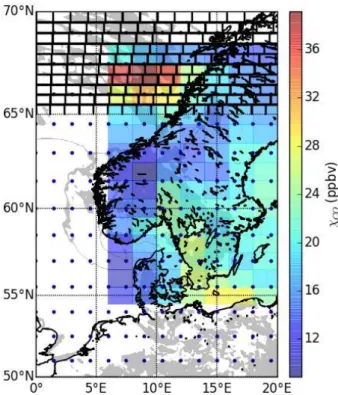
Regarding horizontal co-location, Fig. 2 represents how the datasets are combined. We project data from satellite, model, and reanalysis data sets onto an equal-area

sinu-20

soidal grid such that the grid-cell resolution is 0.5◦×0.5◦ at the equator corresponding to an area of 54 km×54 km. The sinusoidal projection conserves the grid-cell area inde-pendently of longitude and latitude. One grid-cell can include up to 81 POLDER-MODIS pixels. Satellite and tracer transport model data are averaged over each grid-cell.

One consequence of the averaging is that each grid-cell can include up to 81 different

25

pixel-level values ofΦ_{. We place a limit on the SD of the averaged phase index within}

(11)

ACPD

15, 31823–31866, 2015

the Arctic

Q. Coopman et al.

Title Page

Tables Figures

◭ ◮

Back Close

Full Screen / Esc

Discussion

P

a

per

|

Discussion

P

a

per

|

Discussion

P

a

per

|

Discussion

P

a

per

|

3.2 The indirect effect parameter

Assuming a constant LWC and a mono-disperse size distribution of cloud droplets, the droplet eff_{ective radius (r}_e_{) decreases as the droplet number concentration}_N_c

in-creases following the relation (Feingold et al., 2001):

∂lnr_e

∂lnN_c|LWP=− 1

3 (3)

5

Here, we take a different approach which is to examine the sensitivity of clouds properties to the CO tracer under the presumption that the CO tracer serves as a proxy for the potential of pollution, of which CCN may be a part, to modifyNc. Of course,Nc

and CO tracer concentrations (χ_CO) do not represent the same quantity. However, cloud condensation nuclei and CO are both by-products of combustion. The two quantities

10

are expected to be highly correlated close to pollution sources (Avey et al., 2007; Tietze et al., 2011). Thus, the indirect eff_{ect parameter could be expressed alternatively as:}

IE_τ= d lnτ

d lnχ_CO (4)

IE_r

e=−

d lnr_e

d lnχ_CO (5)

15

For example, if N_c, from Eq. (3) is linearly related with χ_CO then Eq. (5) has as its theoretical maximum value of IE_r_e =_1/3.

Further from source regions, the correlation of CO concentration and aerosols is invariant to dilution but it is sensitive to wet and dry scavenging (Garrett et al., 2010, 2011). When aerosol scavenging rates are low, CO and CCN will tend to covary. Values

20

(12)

ACPD

15, 31823–31866, 2015

the Arctic

Q. Coopman et al.

Title Page

Tables Figures

◭ ◮

Back Close

Full Screen / Esc

Discussion

P

a

per

|

Discussion

P

a

per

|

Discussion

P

a

per

|

Discussion

P

a

per

|

exceeds 4◦C at the surface, wet scavenging effi_{ciently removes CCN from the}

atmo-sphere and cloud microphysical properties are not affected by pollution even if the CO remains. Moreover, the simulated CO tracer by the transport model FLEXPART can be de-correlated from the real pollution loading, which can introduce scatter in the results presented here. Effectively, what is expressed by Eq. (4) and (5) is not the sensitivity of

5

clouds to aerosols, but rather their sensitivity to pollution, taking into account the possi-bility that the cloud active component of the polluted air parcel may have been removed. The analysis becomes less focussed on the local physics and more focussed on the actual impact of anthropogenic activities on clouds far from the combustion source.

Sincereand the optical depth (τ) are linked throughτ=3₂LW Pρwre it follows that 10

∂lnτ ∂lnχ_CO =−

∂lnr_e ∂lnχ_CO+

∂ln LWP

∂lnχ_CO (6)

or,

IE_τ=_IE_r

e+IELWP (7)

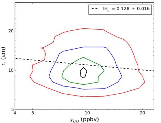
Figure 3 shows an IE retrieval example for temperatures between−12 and 6◦C and altitudes between 1000 and 2000 m, for all LWP values. We first calculate IE_r_e as the

15

linear fit of the natural logarithm of the eff_{ective radius to the natural logarithm of CO}

concentrations. The fit used in this study is based on the robust linear method (RLM) (Huber, 1973, 1981; Venables and Ripley, 2013). RLM uses an iterative least squares algorithm: every measurement has initially the same weight; The weights of each point are updated giving a lower weight to points which appear as outliers with respect to the

20

entire dataset. The process iterates several times and stops when the convergence tolerance of the estimated fitting coeffi_{cients are below 10}−8_{. The slope is therefore}

(13)

ACPD

15, 31823–31866, 2015

the Arctic

Q. Coopman et al.

Title Page

Tables Figures

◭ ◮

Back Close

Full Screen / Esc

Discussion

P

a

per

|

Discussion

P

a

per

|

Discussion

P

a

per

|

Discussion

P

a

per

|

3.3 Constraining IE for specific humidity and lower tropospheric stability

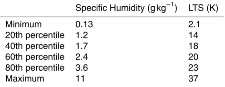
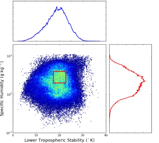
Figure 4 presents a 2-D histogram of frequency distribution of the specific humidity and the LTS. The LTS ranges from 2.1 to 37 K and the specific humidity from 0.13 to 11 g kg−1. The median values for specific humidity and LTS are 2.0 g kg−1 and 19 K respectively.

5

Table 2 describes the method used here for constraining values of IE for meteoro-logical conditions. We identify a range in LTS and specific humidity that occupies 15 % of the total space of observed values but that is centered at the mode of the respective distributions. The total LTS range is 2.1 to 37 K, so the interval size is 5.3 K. Specific humidity is more logarithmically distributed. The logarithm base 10 of specific humidity

10

has an interval of 0.28. The most common values of meteorological state, defined here as the maximum number of measurements, are delimited by the red rectangle in Fig. 4 corresponding to a range between 0.30 and 0.60 for the logarithm of specific humidity, corresponding to a range of 2.0 g kg−1to 4.0 g kg−1, and a range of 16.5 K to 21.8 K for LTS. It is these ranges that are focussed upon for calculation of the IE parameter. We

15

assume these intervals are suffi_{ciently narrow that the variability within the interval has}

limited impact on the cloud microphysics.

4 Results

4.1 The indirect effect

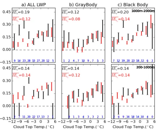
Figure 5 summarizes IE values calculated using combined POLDER-3, MODIS, and

20

FLEXPART data for the period between 2008 and 2010 for latitudes greater than 65◦ over ocean, and constrained for cloud top temperature in bins of 2◦ between−12 and 6◦C. The results are categorized according to bins in temperature, altitude and LWP, and are constrained for LTS and specific humidity. The number of grid-cells used to calculate each IE parameter per bin ranges from 100 to 3300. The IE parameter is

(14)

ACPD

15, 31823–31866, 2015

the Arctic

Q. Coopman et al.

Title Page

Tables Figures

◭ ◮

Back Close

Full Screen / Esc

Discussion

P

a

per

|

Discussion

P

a

per

|

Discussion

P

a

per

|

Discussion

P

a

per

|

almost always positive but sometimes close to zero. IE_r

e ranges from 0 for graybody

clouds between 1000 to 2000 m altitude with a cloud top temperature between−6 and

−4◦C, to 0.34 for blackbody clouds between 1000 and 2000 m altitude with a cloud top temperature between 4 and 6◦C. IE_τ ranges from−0.10 for all clouds between 200 to 1000 m altitude with a cloud top temperature of−11◦C, to 0.35 at 3◦C for blackbody

5

clouds between 1000 and 2000 m altitude. In general, IE_τ and IE_r_e are of the same or-der of magnitude and the maximum values of IE are found for clouds with temperatures above the freezing temperature.

We define the uncertainty in IE as the 95 % confidence limit in the calculation of the slope of the linear fit. The uncertainty in the calculated values of IE_r

e is generally less 10

than 0.1, except for clouds with temperatures between 4 and 6◦C and between −12 and−10◦C where the uncertainty bar is approximately 0.2. For the optical depth, the uncertainty is typically approximately 0.1, although larger values are observed for high and low cloud top temperatures.

For blackbody clouds between 1000 and 2000 m altitude, the average values of IE_τ

15

and IE_r

e equal 0.20 and 0.14 respectively. For cloud tops between 200 and 1000 m

altitude, IE_τ and IE_r_e equal 0.14. For graybody clouds between 1000 and 2000 m, IE_τ and IE_r

e equal 0.12 and 0.08 respectively. For cloud tops between 200 and 1000 m

altitude, IE_τ and IE_r

e equals 0.14 and 0.12 respectively. The value of IE appears to be

fairly robust to altitude and cloud thickness and to whetherr_eorτis considered. Table 3

20

presents the average IE_τ and IE_r

e. In all case cases, values are near 0.13±0.03.

4.2 Dependence of IE on pollution concentration, specific humidity, and lower tropospheric stability

Table 4 shows values of IE_r_e and IE_τ for graybody and blackbody clouds, and for χ_CO<5.5 ppbv and χ_CO>10.0 ppbv, corresponding respectively to the lower and

up-25

(15)

ACPD

15, 31823–31866, 2015

the Arctic

Q. Coopman et al.

Title Page

Tables Figures

◭ ◮

Back Close

Full Screen / Esc

Discussion

P

a

per

|

Discussion

P

a

per

|

Discussion

P

a

per

|

Discussion

P

a

per

|

for IE_r

e than IEτ. Table 4 suggests that cloud effective radius and cloud optical depth

are most sensitive to pollution when pollution concentrations are low. Previous studies have hypothesized that the eff_{ect of CCN on cloud microphysical properties saturates}

when cloud droplet concentrations are high (Bréon et al., 2002; Andersen and Cermak, 2015). This eff_{ect does not explain the di}ff_{erences presented in Table 4 because Eq.} 5

(4) and (5) already take into account the potential for linear saturation by considering the logarithmic values ofχ_CO and cloud parameters.

We now present the sensitivity of the IE parameter to diff_{erent regimes of}

meteoro-logical parameters define by bins delimited by the percentiles presented in Table 5. For each parameter we define 5 diff_{erent regimes – from the bin minimum to 20th percentile} 10

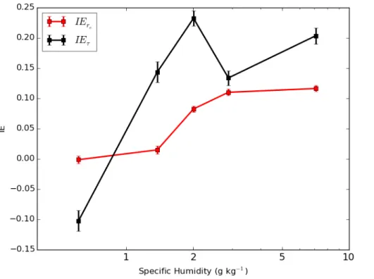
to the bin 80th percentile to maximum. Figures 6 and 7 show the influence of pollution loading on the cloud droplet eff_{ective radius and cloud optical depth for each of the}

diff_{erent specific humidity and LTS regimes. Figure 6 presents the IE parameter with}

respect to the cloud optical depth and cloud droplet eff_{ective radius as a function of the}

specific humidity, constraining for LTS according to the method described in Sect. 3.3.

15

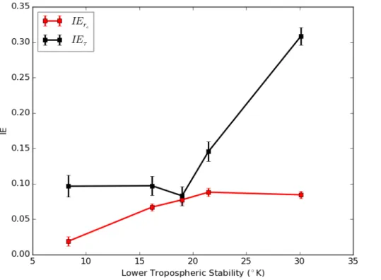
Figure 7 is the same as Fig. 6 except that it shows IE as a function of LTS for a range of specific humidities.

Figure 6 shows that IE_r

e and IEτ tend to increase with the specific humidity

indepen-dent of LTS. The IE parameter is close to zero, or negative, for low values of specific humidity. It increases rapidly with specific humidity, saturating at a maximum value of

20

about 2.5 g kg−1. We note that cloud top temperature and specific humidity are weakly correlated. The correlation coeffi_{cient (r}2_{) of the linear regression of the two parameters}

is 0.20. IE_r

e increases with LTS, from 0.02 for values of LTS ranging between 2.1 and 14 K,

to 0.09 for values of LTS between 23 and 38 K. The IE_τdependance on LTS is larger:

25

(16)

ACPD

15, 31823–31866, 2015

the Arctic

Q. Coopman et al.

Title Page

Tables Figures

◭ ◮

Back Close

Full Screen / Esc

Discussion

P

a

per

|

Discussion

P

a

per

|

Discussion

P

a

per

|

Discussion

P

a

per

|

5 Discussion

The results presented here show values of the IE parameter with respect to the cloud droplet eff_{ective radius and optical depth, for clouds over oceans north of 65}◦ _lying

between 200 and 2000 m, and for the years between 2008 to 2010. We find IE values which range from 0.0 to 0.34 for the cloud droplet eff_{ective radius, and from} ₋_{0.1 to} 5

0.35 for the optical depth.

Prior studies examining the Arctic region have retrieved IE values ranging from−0.10 to 0.40 (Garrett et al., 2004; Lihavainen et al., 2009; Zhao et al., 2012, Sporre et al., 2012). Tietze et al. (2011) calculated IE values ranging from 0.0 to 0.17 using a similar satellite-FLEXPART co-location method presented here. What diff_{ers is that we are} 10

examining solely anthropogenic pollution, we extend the dataset from one to three years, and we constrain for specific humidity and LTS. The larger IE values we find in this study suggest a higher sensitivity of cloud microphysical properties to pollution than was found by Tietze et al. (2011).

However, Tietze et al. (2011) also found values of IE_τ that were greater than IE_r_e,

15

by a factor of up to four, and they attributed this diff_{erence to unknown dynamic or}

precipitation feedbacks that make IE_LWP greater than zero (Eq. 7). In contrast, our results show that the IE_r_e and IE_τ parameters are more similar, suggesting no such feedback. Table 6 compares the diff_{erences between IE}_τ _{and IE}_r

e that are presented

in Table 3, along with their corresponding values when the data are not constrained

20

for specific humidity and LTS. The diff_{erence between IE}_r

e and IEτ is largest when the

data are not constrained for meteorological parameters. For all clouds considered, the maximum diff_{erence increases from 0.04 when the data are constrained to 0.12 when}

the data are not constrained. This is important since it suggests that the hypothesized feedbacks discussed by Tietze et al. (2011) may have in fact been due to the natural

25

sensitivity of clouds to local meteorology. Not constraining suffi_{ciently for meteorology}

(17)

ACPD

15, 31823–31866, 2015

the Arctic

Q. Coopman et al.

Title Page

Tables Figures

◭ ◮

Back Close

Full Screen / Esc

Discussion

P

a

per

|

Discussion

P

a

per

|

Discussion

P

a

per

|

Discussion

P

a

per

|

In contrast to most prior eff_{orts, satellite-retrieved cloud properties are not compared}

to CCN or aerosol concentrations but rather to pollution concentrations – specifically CO simulated from a tracer transport model. For temperatures below−6◦C, low values of IE are observed. Tietze et al. (2011) hypothesized that at such temperatures, cloud supersaturations may be too small to activate aerosols as CCN or that clouds with

5

colder temperatures have followed longer transport pathways nearer the surface (Stohl, 2006) and therefore had greater exposure to dry deposition.

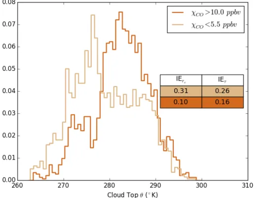
Table 4 suggests that IE values are lowest when pollution concentration is high. Fig-ure 8 presents the normalized distribution of potential temperatFig-ure for polluted and pris-tine clouds, defined as the upper and lower quartile, for graybody clouds. We present

10

results for graybody clouds because the IE diff_{erences between polluted and clean}

cases are largest; Results for blackbody and all clouds are not shown here, but have similar results regarding the potential temperature distribution.

Highly polluted air parcels are associated with potential temperatures around 280 K whereas pristine air parcels have a lower potential temperature – around 272 K. We

15

hypothesize that higher values of potential temperature suggest pollution sources from further south, so wet scavenging is more likely to occur during transport and this de-creases the correlation between CO tracer and CCN, therefore lowering the IE param-eter. Also, polluted air parcel and aerosols do not necessarily have the same physical and chemical properties at lower and higher latitudes, and this diff_{erence may impact} 20

the influence of aerosols on cloud microphysics and aerosols (Bilde and Svenningsson, 2004; Dusek et al., 2006; Ervens et al., 2007; Andreae and Rosenfeld, 2008).

In general, we observe that when the moisture increases, the cloud sensitivity to pollution increases. From model simulations based of stratocumulus Ackerman et al. (2004) found that when the relative humidity (RH) above cloud top is high, cloud LWP

25

increases with Nc consistent with theoretical arguments (Albrecht, 1989; Pincus and

Baker, 1994), but that when the RH is low, the LWP decreases when N_c increases, as supported by some observations (Coakley and Walsh, 2002). The diff_{erence was}

(18)

ACPD

15, 31823–31866, 2015

the Arctic

Q. Coopman et al.

Title Page

Tables Figures

◭ ◮

Back Close

Full Screen / Esc

Discussion

P

a

per

|

Discussion

P

a

per

|

Discussion

P

a

per

|

Discussion

P

a

per

|

common above low-level cloud tops in the Arctic (Nygärd et al., 2014), so similar phe-nomena may be playing a role.

Studies of the indirect eff_{ect at mid-latitudes suggest that values of IE are highest}

under unstable conditions (Chen et al., 2014; Andersen and Cermak, 2015). Our re-sults show that in the Arctic, the impact of LTS on IE is the reverse. Klein and Hartmann

5

(1993) showed that, in general, higher values of LTS lead to greater stratiform cloudi-ness, except in the Arctic where radiative cooling prevails over convection as the driving mechanism for cloud formation.

Finally, we find IE_τ is more sensitive to changes in LTS than IE_r_e. A consequence is that for values of LTS greater than the eightieth percentile bin of 23 K, IE_τ and IE_r

e 10

diff_{er by about 0.20. In a stable atmosphere with high LTS it appears that IE}

LWP

in-creases more strongly in response to aerosols than in unstable environments (Klein and Hartmann, 1993; Qiu et al., 2015).

6 Conclusions

Satellite, numerical model, and meteorological reanalyses data sets from 2008 to 2010

15

have been used here to calculate the sensitivity of cloud droplet eff_{ective radius and}

optical depth in the Arctic to anthropogenic polluted air parcels transported from mid-latitudes. We focussed on latitudes north of 65◦for the period between March 2008 and October 2010. Using ECMWF reanalysis data, we constrained the sensitivity analysis for temperature, LTS, specific humidity, altitude, and LWP. We find values of IE close to

20

the theoretical maximum of 1/3, assuming that a simulated CO tracer correlates well with CCN. IE_r

e and IEτ seem to increase with specific humidity and LTS, highlighting

that meteorological parameters have an important impact on aerosols influence with cloud microphysical properties.

Globally, Klimont et al. (2013) have estimated that there was a drop of about 9281 Gg

25

(19)

ACPD

15, 31823–31866, 2015

the Arctic

Q. Coopman et al.

Title Page

Tables Figures

◭ ◮

Back Close

Full Screen / Esc

Discussion

P

a

per

|

Discussion

P

a

per

|

Discussion

P

a

per

|

Discussion

P

a

per

|

power plants in China. This reduction in emissions has lead to a decrease of sulfate concentrations at Arctic surface station (Hirdman et al., 2010). In the Arctic, the eff_ect

of a decrease in mid-latitude pollution emissions may be some day off_{set by greater}

levels of Arctic industrialization (Lindholt and Glomsrød, 2012) and shipping (Pizzolato et al., 2014; Miller and Ruiz, 2014) that introduce new local aerosol sources. Further,

5

an increase in the extent of open-ocean due to sea-ice retreat may be expected to lead to an increase in the atmospheric humidity (Boisvert and Stroeve, 2015) and from the results presented here, a higher sensitivity of clouds to aerosols. However, this study also suggests that any associated decrease in LTS may be expected to counter-act this eff_{ect. Sea-ice retreat would also enhance dimethyl sulfide emissions, potentially} 10

increasing cloud cover in the Arctic (Ji et al., 2013).

Climate warming is thought to stimulate boreal forest fires (Westerling et al., 2006). The impact of pollution from biomass burning has not been included in the present research. Given biomass burning aerosol can act as effi_{cient ice nuclei (Markus et al.,}

2009), the analyses presented here might be extended to explore aerosol-induced

15

changes in cloud thermodynamic phase.

Acknowledgements. This paper is dedicated posthumously to Kyle Tietze, who developed many of the techniques used in this study while a graduate student at the University of Utah. The authors thank ICARE, NASA and CNES for the data used in this research. We acknowl-edge financial support from The University of Lille1. This material is based upon work supported

20

by the National Science Foundation under the Grant No. 1303965. NILU researchers have re-ceived funding from the European Union Seventh Framework Programme (FP7/2007-2013) under grant agreement no. 282688 – ECLIPSE.

References

Ackerman, A. S., Kirkpatrick, M. P., Stevens, D. E., and Toon, O. B.: The impact of

humid-25

(20)

ACPD

15, 31823–31866, 2015

the Arctic

Q. Coopman et al.

Title Page

Tables Figures

◭ ◮

Back Close

Full Screen / Esc

Discussion

P

a

per

|

Discussion

P

a

per

|

Discussion

P

a

per

|

Discussion

P

a

per

|

Albrecht, B. A.: Aerosols, Cloud Microphysics, and Fractional Cloudiness, Science, 245, 1227– 1230, 1989. 31839

Amann, M., Bertok, I., Borken-Kleefeld, J., Cofala, J., Heyes, C., Höglund-Isaksson, L., Klimont, Z., Nguyen, B., Posch, M., Rafaj, P., Sandler, R., Schöpp, W., Wagner, F., and Winiwarter, W.: Cost-eff_{ective control of air quality and greenhouse gases in}

5

Europe: Modeling and policy applications, Environ. Modell. Softw., 26, 1489–1501, doi:10.1016/j.envsoft.2011.07.012, 2011. 31829

Ancellet, G., Pelon, J., Blanchard, Y., Quennehen, B., Bazureau, A., Law, K. S., and Schwarzen-boeck, A.: Transport of aerosol to the Arctic: analysis of CALIOP and French aircraft data during the spring 2008 POLARCAT campaign, Atmos. Chem. Phys., 14, 8235–8254,

10

doi:10.5194/acp-14-8235-2014, 2014. 31825

Andersen, H. and Cermak, J.: How thermodynamic environments control stratocumulus mi-crophysics and interactions with aerosols, Environ. Res. Lett., 10, 24004, doi:10.1088/1748-9326/10/2/024004, 2015. 31826, 31827, 31837, 31840

Andreae, M. O. and Rosenfeld, D.: Aerosol-cloud-precipitation interactions. Part 1.

15

The nature and sources of cloud-active aerosols, Earth-Sci. Rev., 89, 13–41, doi:10.1016/j.earscirev.2008.03.001, 2008. 31839

Avey, L., Garrett, T. J., and Stohl, A.: Evaluation of the aerosol indirect eff_{ect using}

satel-lite, tracer transport model, and aircraft data from the International Consortium for Atmo-spheric Research on Transport and Transformation, J. Geophys. Res.-Atmos., 112, 1–10,

20

doi:10.1029/2006JD007581, 2007.

Belchansky, G. I., Douglas, D. C., and Platonov, N. G.: Duration of the Arctic sea ice melt season: Regional and interannual variability, 1979-2001, J. Climate, 17, 67–80, doi:10.1175/1520-0442(2004)017<0067:DOTASI>2.0.CO;2, 2004. 31825

Berrisford, P., Dee, D., Fielding, K., Fuentes, M., Kallberg, P., Kobayashi, S., and Uppala, S.: The

25

ERA-Interim Archive, ECMWF, Reading, UK, 1, available at: http://old.ecmwf.int/publications/ library/do/references/list/782009 (last access: 11 November 2015), 2009. 31830

Bilde, M. and Svenningsson, B.: CCN activation of slightly soluble organics: The impor-tance of small amounts of inorganic salt and particle phase, Tellus B, 56, 128–134, doi:10.1111/j.1600-0889.2004.00090.x, 2004. 31839

30

(21)

ACPD

15, 31823–31866, 2015

the Arctic

Q. Coopman et al.

Title Page

Tables Figures

◭ ◮

Back Close

Full Screen / Esc

Discussion

P

a

per

|

Discussion

P

a

per

|

Discussion

P

a

per

|

Discussion

P

a

per

|

Brenguier, J. and Wood, R.: Observational strategies from the micro to meso scale, in: Clouds in the Perturbed Climate System: Their Relationship to Energy Balance, Atmospheric Dy-namics, and Precipitation, edited by: Heintzenberg, J. and Charlson, R. J., 487–510, avail-able at: ftp://ftp-projects.zmaw.de/aerocom/meetings/frankfurt_2007/brenguier.pdf (last ac-cess: 11 November 2015), MIT Press, MASS, Cambridge, 2009. 31826

5

Bréon, F.-M. and Colzy, S.: Cloud detection from the spaceborne POLDER instrument and validation against surface synoptic observations, J. Appl. Meteorol., 38, 777–785, doi:10.1175/1520-0450(1999)038<0777:CDFTSP>2.0.CO;2, 1999. 31828

Bréon, F.-M., Tanré, D., and Generoso, S.: Aerosol effect on cloud droplet size monitored from satellite, Science (New York, N. Y.), 295, 834–8, doi:10.1126/science.1066434, 2002. 31826,

10

31837

Buriez, J. C., Vanbauce, C., Parol, F., Goloub, P., Herman, M., Bonnel, B., Fouquart, Y., Cou-vert, P., and Seze, G.: Cloud detection and derivation of cloud properties from POLDER, Int. J. Remote Sens., 18, 2785–2813, doi:10.1080/014311697217332, 1997. 31828

Chang, F. L. and Coakley, J. A.: Relationships between marine stratus cloud optical depth

15

and temperature: Inferences from AVHRR observations, J. Climate, 20, 2022–2036, doi:10.1175/JCLI4115.1, 2007. 31826

Chen, Y.-C., Christensen, M. W., Stephens, G. L., and Seinfeld, J. H.: Satellite-based estimate of global aerosol–cloud radiative forcing by marine warm clouds, Nat. Geosci., advance on, 7, 643–646, doi:10.1038/ngeo2214, 2014. 31827, 31840

20

Coakley, J. A. and Walsh, C. D.: Limits to the aerosol indirect radiative eff_ect

de-rived from observations of ship tracks, J. Atmos. Sci., 59, 668–680, doi:10.1175/1520-0469(2002)059<0668:LTTAIR>2.0.CO;2, 2002. 31839

Costantino, L. and Bréon, F. M.: Aerosol indirect effect on warm clouds over South-East At-lantic, from co-located MODIS and CALIPSO observations, Atmos. Chem. Phys., 13, 69–88,

25

doi:10.5194/acp-13-69-2013, 2013. 31826

Dee, D. P., Uppala, S. M., Simmons, A. J., Berrisford, P., Poli, P., Kobayashi, S., Andrae, U., Balmaseda, M. A., Balsamo, G., Bauer, P., Bechtold, P., Beljaars, A. C. M., van de Berg, L., Bidlot, J., Bormann, N., Delsol, C., Dragani, R., Fuentes, M., Geer, A. J., Haimberger, L., Healy, S. B., Hersbach, H., Hólm, E. V., Isaksen, L., Kållberg, P., Köhler, M., Matricardi, M.,

30

(22)

ACPD

15, 31823–31866, 2015

the Arctic

Q. Coopman et al.

Title Page

Tables Figures

◭ ◮

Back Close

Full Screen / Esc

Discussion

P

a

per

|

Discussion

P

a

per

|

Discussion

P

a

per

|

Discussion

P

a

per

|

performance of the data assimilation system, Q. J. Roy. Meteorol. Soc., 137, 553–597, doi:10.1002/qj.828, 2011. 31830

Desmons, M., Ferlay, N., Parol, F., Mcharek, L., and Vanbauce, C.: Improved information about the vertical location and extent of monolayer clouds from POLDER3 measurements in the oxygen A-band, Atmos. Meas. Tech., 6, 2221–2238, doi:10.5194/amt-6-2221-2013, 2013.

5

31828

Dusek, U., Frank, G. P., Hildebrandt, L., Curtius, J., Schneider, J., Walter, S., Chand, D., Drewnick, F., Hings, S., Jung, D., Borrmann, S., and Andreae, M. O.: Size matters more than chemistry for cloud-nucleating ability of aerosol particles, Science (New York, N. Y.), 312, 1375–1378, doi:10.1126/science.1125261, 2006. 31839

10

Eckhardt, S., Quennehen, B., Olivié, D. J. L., Berntsen, T. K., Cherian, R., Christensen, J. H., Collins, W., Crepinsek, S., Daskalakis, N., Flanner, M., Herber, A., Heyes, C., Hodnebrog, Ø., Huang, L., Kanakidou, M., Klimont, Z., Langner, J., Law, K. S., Lund, M. T., Mahmood, R., Massling, A., Myriokefalitakis, S., Nielsen, I. E., Nøjgaard, J. K., Quaas, J., Quinn, P. K., Raut, J.-C., Rumbold, S. T., Schulz, M., Sharma, S., Skeie, R. B., Skov, H., Uttal, T., von

15

Salzen, K., and Stohl, A.: Current model capabilities for simulating black carbon and sul-fate concentrations in the Arctic atmosphere: a multi-model evaluation using a comprehen-sive measurement data set, Atmos. Chem. Phys., 15, 9413–9433, doi:10.5194/acp-15-9413-2015, 2015. 31830

Ervens, B., Cubison, M., Andrews, E., Feingold, G., Ogren, J. A., Jimenez, J. L., DeCarlo, P.,

20

and Nenes, A.: Prediction of cloud condensation nucleus number concentration using mea-surements of aerosol size distributions and composition and light scattering enhancement due to humidity, J. Geophys. Res.-Atmos., 112, 1–15, doi:10.1029/2006JD007426, 2007. 31839

Feingold, G.: Modeling of the first indirect eff_{ect: Analysis of measurement requirements,}

Geo-25

phys. Res. Lett., 30, 30, 1997, doi:10.1029/2003GL017967, 2003a. 31826

Feingold, G.: First measurements of the Twomey indirect eff_{ect using ground-based remote}

sensors, Geophys. Res. Lett., 30, 19–22, doi:10.1029/2002GL016633, 2003b. 31825 Feingold, G., Remer, L. A., Ramaprasad, J., and Kaufman, Y. J.: Analysis of smoke impact on

clouds in Brazilian biomass burning regions: An extension of Twomey’s approach, J.

Geo-30

(23)

ACPD

15, 31823–31866, 2015

the Arctic

Q. Coopman et al.

Title Page

Tables Figures

◭ ◮

Back Close

Full Screen / Esc

Discussion

P

a

per

|

Discussion

P

a

per

|

Discussion

P

a

per

|

Discussion

P

a

per

|

Fougnie, B., Bracco, G., Lafrance, B., Ruff_{el, C., Hagolle, O., and Tinel, C.: PARASOL}

in-flight calibration and performance, Appl. Optics, 46, 5435–5451, doi:10.1364/AO.46.005435, 2007. 31828

Garrett, T. J. and Zhao, C.: Increased Arctic cloud longwave emissivity associated with pollution from mid-latitudes, Letters, 440, 787–789, doi:10.1038/nature04636, 2006. 31825, 31831,

5

31832

Garrett, T. J., Radke, L. F., and Hobbs, P. V.: Aerosol Eff_{ects on Cloud Emissivity and}

Surface Longwave Heating in the Arctic, J. Atmos. Sci., 59, 769–778, doi:10.1175/1520-0469(2002)059<0769:AEOCEA>2.0.CO;2, 2002. 31825

Garrett, T. J., Zhao, C., Dong, X., Mace, G. G., and Hobbs, P. V.: Eff_{ects of}

vary-10

ing aerosol regimes on low-level Arctic stratus, Geophys. Res. Lett., 31, L17105, doi:10.1029/2004GL019928, 2004. 31825, 31832, 31838

Garrett, T. J., Maestras, M. M., Krueger, S. K., and Shmidt, C. T.: Acceleration by aerosol of a radiative-thermodynamic cloud feedback influencing Arctic surface warming, Geophys. Res. Lett., 36, L19804, doi:10.1029/2009GL040195, 2009. 31831

15

Garrett, T. J., Zhao, C., and Novelli, P. C.: Assessing the relative contributions of transport effi_{ciency and scavenging to seasonal variability in Arctic aerosol, Tellus B, 62, 190–196,}

doi:10.1111/j.1600-0889.2010.00453.x, 2010. 31825, 31833

Garrett, T. J., Brattström, S., Sharma, S., Worthy, D. E. J., and Novelli, P.: The role of scavenging in the seasonal transport of black carbon and sulfate to the Arctic, Geophys. Res. Lett., 38,

20

L16805, doi:10.1029/2011GL048221, 2011. 31833

Hirdman, D., Sodemann, H., Eckhardt, S., Burkhart, J. F., Jeff_{erson, A., Me}ff_{ord, T., Quinn, P. K.,}

Sharma, S., Ström, J., and Stohl, A.: Source identification of short-lived air pollutants in the Arctic using statistical analysis of measurement data and particle dispersion model output, Atmos. Chem. Phys., 10, 669–693, doi:10.5194/acp-10-669-2010, 2010. 31830, 31841

25

Huber, P. J.: The 1972 Wald memorial lectures: robust regression: asymptotics, conjectures, and Monte Carlo, The Annals of Statistics, 1, 799–821, 1973. 31834

Huber, P. J.: Robust Statistics, John Wiley and Sons, Inc., New York, 1981. 31834

Ji, R., Jin, M., and Varpe, Ø.: Sea ice phenology and timing of primary production pulses in the Arctic Ocean, Glob. Change Biol., 19, 734–741, doi:10.1111/gcb.12074, 2013. 31841

30

Kaufman, Y. J., Koren, I., Remer, L. A., Rosenfeld, D., and Rudich, Y.: The eff_{ect of smoke, dust,}

(24)

ACPD

15, 31823–31866, 2015

the Arctic

Q. Coopman et al.

Title Page

Tables Figures

◭ ◮

Back Close

Full Screen / Esc

Discussion

P

a

per

|

Discussion

P

a

per

|

Discussion

P

a

per

|

Discussion

P

a

per

|

Kawamoto, K., Hayasaka, T., Uno, I., and Ohara, T.: A correlative study on the relationship between modeled anthropogenic aerosol concentration and satellite-observed cloud proper-ties over east Asia, J. Geophys. Res.-Atmos., 111, 1–7, doi:10.1029/2005JD006919, 2006. 31826

Kim, B. G., Miller, M. A., Schwartz, S. E., Liu, Y., and Min, Q.: The role of adiabaticity in the

5

aerosol first indirect eff_{ect, J. Geophys. Res.-Atmos., 113, 1–13, doi:10.1029/2007JD008961,}

2008. 31826

King, M. D. and Platnick, S.: Collection 005 change summary for the MODIS cloud optical property (06 _ OD) algorithm high impact change overview: change details:, Terra, 1, 1–23, 2006. 31828

10

Klein, S. A. and Hartmann, D. L.: The seasonal cycle of low stratiform clouds, J. Climate, 6, 1587–1606, 1993.

Klimont, Z., Smith, S. J., and Cofala, J.: The last decade of global anthropogenic sulfur dioxide: 2000–2011 emissions, Environ. Res. Lett., 8, 014003, doi:10.1088/1748-9326/8/1/014003, 2013. 31840

15

Klimont, Z., Hoglund, L., Heyes, C., Rafaj, P., Schoepp, W., Cofala, J., Borken-Kleefeld, J., Purohit, P., Kupiainen, K., Winiwarter, W., Amann, M., Zhao, B., Wang, S. X., Bertok, I., and Sander, R.: Global scenarios of air pollutants and methane: 1990–2050, in preparation, 2015. 31829

Lance, S., Shupe, M. D., Feingold, G., Brock, C. A., Cozic, J., Holloway, J. S., Nenes, A.,

20

Schwartz, J. P., Spackman, J. R., Froyd, K. D., Murphy, D. M., Brioude, J., Cooper, O. R., Stohl, A., and Burkhart, J. F.: Cloud condensation nuclei as a modulator of ice processes in Arctic mixed-phase clouds, Atmos. Chem. Phys., 11, 8003–8015, 2011,

http://www.atmos-chem-phys.net/11/8003/2011/. 31825

Law, K. S. and Stohl, A.: Arctic air pollution: origins and impacts, Science (New York, N. Y.),

25

315, 1537–40, doi:10.1126/science.1137695, 2007. 31825

Law, K. S., Stohl, A., Quinn, P. K., Brock, C., Burkhart, J., Paris, J. D., Ancellet, G., Singh, H. B., Roiger, A., Schlager, H., Dibb, J., Jacob, D. J., Arnold, S. R., Pelon, J., and Thomas, J. L.: Arctic air pollution: new insights from POLARCAT-IPY, B. Am. Meteorol. Soc., 95, 1873–1895, doi:10.1175/BAMS-D-13-00017.1, 2014. 31825

30

(25)

ACPD

15, 31823–31866, 2015

the Arctic

Q. Coopman et al.

Title Page

Tables Figures

◭ ◮

Back Close

Full Screen / Esc

Discussion

P

a

per

|

Discussion

P

a

per

|

Discussion

P

a

per

|

Discussion

P

a

per

|

Lindholt, L. and Glomsrød, S.: The Arctic: No big bonanza for the global petroleum industry, Energ. Econ., 34, 1465–1474, doi:10.1016/j.eneco.2012.06.020, 2012. 31841

Lohmann, U. and Feichter, J.: Global indirect aerosol eff_{ects: a review, Atmos. Chem. Phys., 5,}

715–737, doi:10.5194/acp-5-715-2005, 2005. 31826

Longley, I. D., Inglis, D. W. F., Gallagher, M. W., Williams, P. I., Allan, J. D., and

5

Coe, H.: Using NO_x and CO monitoring data to indicate fine aerosol number concen-trations and emission factors in three UK conurbations, Atmos. Environ., 39, 5157–5169, doi:10.1016/j.atmosenv.2005.05.017, 2005. 31826

Lubin, D. and Vogelmann, A. M.: A climatologically significant aerosol longwave indirect effect in the Arctic, Nature, 439, 453–456, doi:10.1038/nature04449, 2006. 31831, 31832

10

Lubin, D. and Vogelmann, A. M.: Expected magnitude of the aerosol shortwave indi-rect eff_{ect in springtime Arctic liquid water clouds, Geophys. Res. Lett., 34, L11801,}

doi:10.1029/2006GL028750, 2007. 31825

Markus, T., Stroeve, J. C., and Miller, J.: Recent changes in Arctic sea ice melt onset, freezeup, and melt season length, J. Geophys. Res.-Oceans, 114, 1–14, doi:10.1029/2009JC005436,

15

2009. 31825, 31841

Matsui, T., Masunaga, H., Kreidenweis, S. M., Pielke, R. A., Tao, W. K., Chin, M., and Kauf-man, Y. J.: Satellite-based assessment of marine low cloud variability associated with aerosol, atmospheric stability, and the diurnal cycle, J. Geophys. Res.-Atmos., 111, 1–16, doi:10.1029/2005JD006097, 2006. 31831

20

Mauger, G. S. and Norris, J. R.: Meteorological bias in satellite estimates of aerosol-cloud relationships, Geophys. Res. Lett., 34, 1–5, doi:10.1029/2007GL029952, 2007. 31831 Mauritsen, T., Sedlar, J., Tjernström, M., Leek, C., Martin, M., Shupe, M., Sjogren, S., Sierau, B.,

Persson, P. O. G., Brooks, I. M., and Swietlicki, E.: An Arctic CCN-limited cloud-aerosol regime, Atmos. Chem. Phys., 11, 165–173, 2011,

25

http://www.atmos-chem-phys.net/11/165/2011/. 31831, 31832

Miller, A. W. and Ruiz, G. M.: Arctic shipping and marine invaders, Nature Clim. Change, 4, 413–416, doi:10.1038/nclimate2244, 2014. 31841

Myhre, G., Stordal, F., Johnsrud, M., Kaufman, Y. J., Rosenfeld, D., Storelvmo, T., Kristjansson, J. E., Berntsen, T. K., Myhre, A., and Isaksen, I. S. A.: Aerosol-cloud interaction inferred

30

(26)

ACPD

15, 31823–31866, 2015

the Arctic

Q. Coopman et al.

Title Page

Tables Figures

◭ ◮

Back Close

Full Screen / Esc

Discussion

P

a

per

|

Discussion

P

a

per

|

Discussion

P

a

per

|

Discussion

P

a

per

|

Nakajima, T., Higurashi, A., Kawamoto, K., and Penner, J. E.: A possible correlation between satellite-derived cloud and aerosol microphysical parameters, Geophys. Res. Lett., 28, 1171– 1174, doi:10.1029/2000GL012186, 2001. 31826

Nygärd, T., Valkonen, T., and Vihma, T.: Characteristics of arctic low-tropospheric humidity inversions based on radio soundings, Atmos. Chem. Phys., 14, 1959–1971,

doi:10.5194/acp-5

14-1959-2014, 2014. 31840

Overland, J. E. and Wang, M.: When will the summer Arctic be nearly sea ice free?, Geophys. Res. Lett., 40, 2097–2101, doi:10.1002/grl.50316, 2013. 31825

Painemal, D., Kato, S., and Minnis, P.: Boundary layer regulation in the southeast Atlantic cloud microphysics during the biomass burning season as seen by the A-train satellite

con-10

stellation, J. Geophys. Res.-Atmos., 119, 11288–11302, doi:10.1002/2014JD022182, 2014. 31826

Paris, J.-D., Stohl, A., Nédélec, P., Arshinov, M. Yu., Panchenko, M. V., Shmargunov, V. P., Law, K. S., Belan, B. D., and Ciais, P.: Wildfire smoke in the Siberian Arctic in summer: source characterization and plume evolution from airborne measurements, Atmos. Chem. Phys., 9,

15

9315–9327, doi:10.5194/acp-9-9315-2009, 2009. 31830

Pincus, R. and Baker, M. B.: Eff_{ect of precipitation on the albedo susceptibility of clouds in the}

marine boundary layer, Nature, 372, 250–252, doi:10.1038/372250a0, 1994. 31839

Pizzolato, L., Howell, S. E. L., Derksen, C., Dawson, J., and Copland, L.: Changing sea ice conditions and marine transportation activity in Canadian Arctic waters between 1990 and

20

2012, Climatic Change, 123, 161–173, doi:10.1007/s10584-013-1038-3, 2014. 31841 Platnick, S., King, M. D., Ackerman, S. A., Menzel, W. P., Baum, B. A., Riédi, J. C., and

Frey, R. A.: The MODIS cloud products: Algorithms and examples from terra, IEEE T. Geosci. Remote, 41, 459–472, doi:10.1109/TGRS.2002.808301, 2003. 31828

Qiu, S., Dong, X., Xi, B., and Li, J. F.: Characterizing Arctic mixed-phase cloud structure and

25

its relationship with humidity and temperature inversion using ARM NSA observations, J. Geophys. Res., 120, 7737–7746, doi:10.1002/2014JD023022.Received, 2015. 31840 Quinn, P. K., Shaw, G., Andrews, E., Dutton, E. G., Ruoho-Airola, T., and Gong, S. L.:

Arc-tic haze: Current trends and knowledge gaps, Tellus B, 59, 99–114, doi:10.1111/j.1600-0889.2006.00238.x, 2007. 31825

30

Richter-Menge, J. and Jeff_{ries, M.: State of the climate in 2010: The Arctic, B. Am. Meteorol.}