Survey of propagation Model in wireless Network

Survey of propagation Model in wireless Network

1

Hemant kumar sharma, 2sanjeev Sharma, 3Krishna Kumar Pandey 1

School of IT, Rajiv Gandhi Proudyogiki Vishwavidyalaya, Bhopal (M.P.)India

2

School of IT, Rajiv Gandhi Proudyogiki Vishwavidyalaya, Bhopal (M.P.) 462036, India

2

School of IT, Rajiv Gandhi Proudyogiki Vishwavidyalaya, Bhopal (M.P.) 462036, India

Abstract

To implementation of mobile ad hoc network wave propagation models are necessary to determine propagation characteristic through a medium. Wireless mobile ad hoc networks are self creating and self organizing entity. Propagation study provides an estimation of signal characteristics. Accurate prediction of radio propagation behaviour for MANET is becoming a difficult task. This paper presents investigation of propagation model. Radio wave propagation mechanisms are absorption, reflection, refraction, diffraction and scattering. This paper discuss free space model, two rays model, and cost 231 hata and its variants and fading model, and summarized the advantages and disadvantages of these model. This study would be helpful in choosing the correct propagation model.

Keywords

:

mobile ad hoc network, propagation mechanism, path loss, propagation model and fading model.

1.

I

NTRODUCTION

Commercial success of MANET, since its initial implementation in the early 1972, has lad to an interest between wireless engineers in understanding and predicting radio propagation characteristic in different urban and suburban area, expansive growth of MANET, it is very precious to have the capability of determining path loss. An ad hoc network [2] is a collection of wireless movable nodes (or routers) dynamically forming a temporary network without the use of any existing network infrastructure or centralized administration. The routers are free to move randomly and organize themselves arbitrarily; thus, the network’s wireless topology may change rapidly and unpredictably. it have potential use in a wide variety of disparate situations such as responses to storm, tsunami, volcanic activity, disaster relief, terrorism and military operations. This work investigation on behaviour of different propagation model in MANET, propagation models [4][10] are divided into three types of models that are the empirical models, semi-deterministic models and deterministic models. Empirical models are depends on measurement data, statistical properties and few parameters. Examples of empirical models are Okumura model and Hata model. Semi-deterministic models are based on empirical models and deterministic aspects, examples being the Cost-231 and Walficsh-Ikegami. Deterministic models are site-specific, requires huge

number of geometry information about the city, computational effort and more ideal model. A fading model [14] calculates the effect of changes in characteristics of the propagation path on the signal strength, fading models are three types: Rayleigh and ricean fading model.

In the next section brief overview of path loss, section III discusses propagation mechanism, section IV describe propagation model, section V discuss fading model and last section is conclusion.

2.

PATH LOSS

Path loss[7] (PL) is a measure of the average RF

attenuation difference between transmitted signals when it arrives at the receiver, after traversing a path of several wavelengths. It is defined by [8]

2 .

2 2

. . ( )

( 4 )

t t r

r

P G G

P d

d L  



(

)

10 log

t

L

r

P

P dB

P



(1) where Pt and pr are the transmitted and received power. In free space, the power reaching the receiving antenna which is separated from the transmitting antenna by a distance d is given by the Friis free-space equation:

2 . 2 2

. .

( )

( 4 )

t t r

r

P G G

P

d

d L







(2) Where Gt and Gr, are gain of transmitting and receiving antenna, respectively. L is the system loss factor, not related to propagation. λis the wavelength in meters.

3.

PROPAGATION MECHANISM

There are some propagation mechanisms [12] that effect propagation in mobile ad hoc network. They are explained in this section.

Absorption

energy occurs at the molecular level, resulting from the interaction of the energy of the radio wave and the material of the medium or obstacle

Refraction

Refraction occurs when a radio wave passes from one medium to another with different refractive indices resulting in a change of velocity within an electromagnetic wave that results in a change of direction.

Reflection

Reflection [8][12] occurs when a propagating electromagnetic wave impinges upon an object that has very large dimensions compared to the wavelength of the propagating wave. Reflection occurs from the surface of the ground, from walls, and from furniture.

Fig. 1 reflection and refraction

Diffraction

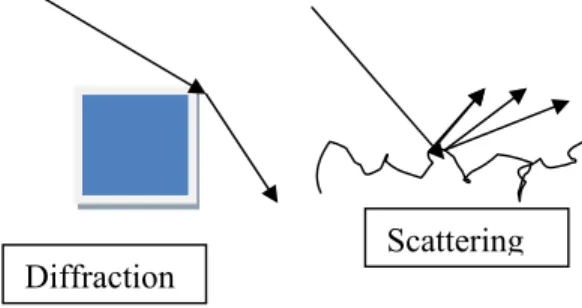
Diffraction losses [6] occur when there is an obstacle in the path of the radio wave transmission and the radio waves either bend around an object or spread as they pass through an opening. Diffraction can cause great levels of attenuation at high frequencies. However, at low frequencies, diffraction actually extends the range of the radio transmission.

Fig. 2 Diffraction and scattering Scattering

Scattering is a condition that occurs when a radio wave encounters small disturbances of a medium, which can alter the direction of the signal. Certain weather phenomena such as rain, snow, and hail can cause scattering of a transmitted radio wave. Scattering is difficult to predict because of the random nature of the medium or objects that cause it.

4.

PROPAGATION

MODEL

4.1 free space path loss model

This is a large scale model. The received power is only dependent on the transmitted power, the antenna’s gains and on the distance between the sender and the receiver. It accounts mainly for the fact that a radio wave which moves away from the sender has to cover a larger area. So the received power decreases with the square of the distance. The free space propagation model assumes the ideal propagation condition that there is only one clear line-of-sight path between the transmitter and receiver. H. T. Friis presented the following equation to calculate the received signal power in free space at distance d from the transmitter [5] [13].

Where PT is the transmitted signal power GT and GR are the antenna gains of the transmitter and the receiver

respectively.



is the wavelength. It is common to select GT = GR =1.then,

Expressed in dB as:

=

One is able to see from the above free space equations that 6 dB of loss is associated with a doubling of the frequency. This same relationship also holds for the distance, if the distance is doubled, 6 dB of additional loss will be encountered.

4.2 Two Ray Ground Model

One more popular path loss model is the two-ray model or the two-path model. The free space model described above assumes that there is only one single path from the transmitter to the receiver. But in reality the signal reaches the receiver through multiple paths (because of reflection, refraction and scattering). The two-path model tries to capture this phenomenon. The model assumes that the signal reaches the receiver through two paths, one a line-of-sight path, and the other the path through which the reflected wave is received. According to the two-path model, the received power is given by [8],

 

……….. (4)

Where Pt is the transmitted power, Gt and Gr are the transmitter and receiver antenna gains, respectively, in the direction from the transmitter and receiver, d is the distance between the transmitter and receiver, and ht and hr are the heights of the transmitter and receiver, respectively.

4.3 okumara Model

Okumara is the first model to find path loss in urban area. Okumura’s model [3] [11] is most widely used for signal

Diffraction

Scattering

Incoming RF

Refracted RF Reflected

predictions in urban and suburban areas operating in the range of 150MHz to 1.92 GHz. The basis of the method is that the free space path loss between the transmitter and receiver is added to the value of Amu(f,d),where Amu isthe median attenuation, relative to free space in an urban area with a base station effective antenna height Hte 200meter and mobile station height Hre is 3 meter To determine path loss using Okumura’s model, the free space path loss between the points of interest is first determined, and then the value of Amu (f, d) is added to it along with correction factors to account for the type of terrain as expressed in.

        –      ………..(5) Here, L50(dB) is the 50 percentile value of propagation path loss, LF is propagation loss of free space, Amu is the median attenuation relative to free space, GHte , GHre , Garea are BTS antenna height gain factor, mobile antenna height gain factor and gain due to the type of environment. Okumara model is empirical in nature means that all parameters all parameters are used to specific range determined by the measured data.if the user finds that one or more parameters are outside the range then there is no alternate. Limitation of this model is its slow response to quick changes in terrain.

4.4 Hata model

The The Hata model is an empirical formulation [7] of the graphical path-loss data provided by Okumura’s model. The formula for the median path loss in urban areas is given by

      .   . log .          .     .     .

……..(6) Where fcis the frequency (in MHz), which varies from 150

MHz to 1500MHz hte and hre are the effective heights of the base station and the mobile antennas (in meters), respectively. d is the distance from the base station to the mobile antenna, a(hre) is the correction factor for the effective antenna height of the mobile unit, which is a function of the size of the area of coverage. For small- to medium-sized cities, the mobile-antenna correction factor is given by:

. . . .

Path loss in suburban area

  .

The path loss in open rural area as is expressed

  . . .

These equation improved performance value of okumara model, this technique is good in urban and suburban area but in rural areas performance degreases because rural area prediction is depend on urban area. This model is quite suitable for large-cell mobile systems, but not for personal communications systems that cover a circular area of approximately 1 kmin radius.

4.5 Cost 231 Walfisch Ikagami Model

This empirical model is a combination of the models from J. Walfisch and F. Ikegami. It was developed by the COST 231 project. It is now called Empirical COST-Walfisch-Ikegami Model. The frequency ranges from 800MHz to 2000 MHz. This model is used primarily in Europe for the GSM1900 system [1] [11]

Path Loss,

………. (7) Where

Lf = free-space loss

Lrts = rooftop-to-street diffraction and scatter loss Lmsd = multi screen loss

Free space loss is given as

.

The rooftop-to-street diffraction and scatter loss is given as [13]

  . log    

log   log∆    

  .               

. .        

. .        

With w = width of the roads Where Lori = Orientation Loss

φ= incident angle relative to the street The multi screen loss is given as:

 

 

log

  log

log

Where

log  ∆          

               

 

                . ∆          .      

. ∆ /_{.       r d    .  km}

 

             ∆            

k

   

. f Mhz  for medium sized city and suburban 

. f Mhz  _{for mertopolitan centers}       

station height is 1 to 3 m, and distance between base station and mobile station d is 0.02 to 5km.

5. FADING MODEL

Fading [14] is variation of the attenuation that a carrier-modulated telecommunication signal experiences above certain transmission medium. The fading may vary with time, environmental location or radio frequency, and is often modelled as arbitrary process. In wireless systems, fading may either be due to multipath propagation, or due to shadowing from obstacles affecting the wave propagation, referred to as shadow fading. The presence of reflectors in the environment surrounding a transmitter and receiver create multiple paths that a transmitted signal can traverse. As a result, the receiver sees the superposition of multiple copies of the transmitted signal, each traversing a different path. Each signal copy will experience differences in attenuation, delay and phase shift while travelling from the source to the receiver.

5.1RAYLEIGH Fading

Rayleigh fading is a geometric model for the effect of a propagation situation on a radio signal. Rayleigh fading is described as a realistic model for tropospheric and ionospheric signal propagation as well as the effect of heavily built-up metropolitan environments on radio signals. Rayleigh fading is most applicable when there is no dominant propagation along a line of sight (LOS) between the transmitter and receiver. If there is a dominant LOS, Rician fading may be more suitable. Rayleigh fading is a practical model when there are various objects in the environment that spread the radio signal before it comes at the receiver. The central limit theorem holds that, if there is sufficiently much spread, the channel impulse response will be well-modelled as a Gaussian process irrespective of the distribution of the individual components. If there is no dominant component to the scatter, then such a process will have zero mean and phase evenly distributed between 0 and 2π radians. This random variable R, it will have a probability density function

………… (9) where Ω = E(R2)

Often, the gain and phase elements of a channel's distortion are conveniently represented as a complex number.

Fig. 3 Rayleigh Fading 5.2 Racian fading

It is a stochastic model for radio propagation anomaly caused by partial cancellation of a radio

signal by itself

signal arrives at the receiver by two different paths, and at least one of the paths is changing. Rician fading occurs when one of the paths, usually a

LOS signal, is much

stronger than the others. In Rician fading, the amplitude gain is characterized by a

Rician distribution.

Rayleigh fading is the precise model for stochastic

fading when there is no LOS signal, and is sometimes considered as a special case of the more general concept of Rician fading. In this fading amplitude gain is characterized by a

Rayleigh distribution. A Ricean

fading channel described by two parameters: K and Ω. K is the ratio between the power in the direct path and the power in the other, scattered, paths. Ω is the power in the direct path, and acts as a scaling factor to the distribution. The received signal amplitude R is then Rice

distributed with parameters

And

The resulting PDF then is

Where

is the Zeroth order modified Bessel function of the first kind.

6.

C

ONCLUSIONS

This paper study some propagation model and fading model and also describes two main characteristic of wireless channel path loss and fading. Propagation model depends on the transmitter height, when transmitter height is high okumara and cost 231 wi model are perform better. But when transmitter height is below to roof height prediction of these models is poor. The accuracy of every model in any given condition will depend on the suitability among parameter required by the model and available terrain, no single model is generally acceptable as the best.

REFERENCES

[1]. R. Mardeni and K. F. Kwan “Optimization of Hata Propagation Prediction Model in Suburban Area In Malaysia” Progress In Electromagnetics Research C, Vol. 13, 91106,2010.

[2]. Ayyaswamy Kathirvel, and Rengaramanujam Srinivasan “Analysis of Propagation Model using Mobile Ad Hoc Network Routing Protocols” International Journal of Research and Reviews in Computer Science (IJRRCS), Vol. 1, No. 1, 2010. [3]. Sagar Patel, Ved Vyas Dwivedi and Y.P. Kosta

prediction Models for Wireless Environment” Number 4 (2010).

[4]. Nagendra sah and Amit Kumar “CSP Algorithm in Predicting and Optimizing the Path Loss of Wireless Empirical Propagation Models” International Journal of Computer and Electrical Engineering, Vol. 1, No. 4, October, 2009. [5]. Ibrahim Khider Eltahir “The Impact of Different

Radio Propagation Models for Mobile Ad hoc Networks (MANET) in Urban Area Environment” The 2nd International Conference on Wireless Broadband and Ultra Wideband Communications (Aus Wireless 2007).

[6]. H. Sizun, P.de Fornel, “Radio Wave Propagation for Telecommunication Applications”, Springer, ISBN: 978-3540407584, 2004.

[7]. Tapan K. Sarkar, Zhong Ji, Kyungjung Kim, Abdellatif Medour “A Survey of Various Propagation Models for Mobile Communication”

IEEE Antennas and Propagation Magazine, Vol. 45, No. 3, June 2003.

[8]. Thomas kurner “propagation prediction models” chapter 4 pp115-116, 2002.

[9]. Theodore S. Rappaport,, Wireless

Communications: Principles and Practice, Prentice Hall PTR,2002.

[10]. H.L. Bertoni, “radio propagation for morden wireless systems”, upper saddle river, nj, prentice Hall PTR, pp 90-92,2000.

[11]. J. D. Parsons “The Mobile Radio Propagation Channel” Chepter1 & 4 pp 4- 7John wiley and son’s ltd 2000.

[12]. Ian Poole, “Radio Signal Path Loss,” n.d.

[13]. James Demetriou and Rebecca MacKenzie “Propagation Basics” September 30, 1998.