Individual heterogeneity and identifiability in capture-recapture models

© 2004 Museu de Ciències Naturals ISSN: 1578–665X

Link, W. A., 2004. Individual heterogeneity and identifiability in capture–recapture models. Animal Biodiversity and Conservation, 27.1: 87–91.

Abstract

Individual heterogeneity and identifiability in capture–recapture models.— Individual heterogeneity in detec-tion probabilities is a far more serious problem for capture–recapture modeling than has previously been recognized. In this note, I illustrate that population size is not an identifiable parameter under the general closed population mark–recapture model M_h. The problem of identifiability is obvious if the population includes individuals with p_i = 0, but persists even when it is assumed that individual detection probabilities are bounded away from zero. Identifiability may be attained within parametric families of distributions for p_i, but not among parametric families of distributions. Consequently, in the presence of individual heterogeneity in detection probability, capture–recapture analysis is strongly model dependent.

Key words: Capture–recapture, Detection probability, Heterogeneity, Identifiability, Population estimation. Resumen

Heterogeneidad individual e identificabilidad en modelos de captura–recaptura.— La heterogeneidad individual en las probabilidades de detección representa un problema para la modelación del procedimiento de captura–recaptura mucho más serio de lo que previamente se había reconocido. En este artículo se demuestra que el tamaño de la población no constituye un parámetro identificable en el modelo general M_h que emplea técnicas de marcaje–recaptura de poblaciones cerradas. El problema de la identificabilidad resulta evidente si la población incluye individuos con p_i = 0, pero sigue persistiendo aun cuando se presuponga que las probabilidades de detección individual se han alejado de cero. La identificabilidad puede conseguirse en familias paramétricas de distribuciones para p_i, pero no entre familias paramétricas de distribuciones. Por consiguiente, si se da una heterogeneidad individual en la probabilidad de detección, el análisis de captura–recaptura depende considerablemente del modelo considerado.

Palabras clave: Captura–recaptura, Probabilidades de detección, Heterogeneidad, Identificabilidad, Estimación de la población.

William A. Link, USGS Patuxent Wildlife Research Center, 11510 American Holly Drive, Laurel, Maryland 20708 U.S.A.

Individual heterogeneity and

identifia bility in

ca pture–reca pture models

I nt roduc t ion

Let X_i, i = 1,2,...,N be independent binomial random variables, with common index T and success rates p_i sampled independently from distribution g(p). Further, let

where 1(·) is the indicator function. Having ob-served f c_{= (f}

1,f2,...,fT), the problem is to estimate N,

or equivalently, to predict f₀. This is the closed population capture–recapture model M_h: N is the unknown population size, X_i is the number of times animal i is captured in T sampling occasions, f_j is the number of animals captured exactly j times.

Numerous methods for estimating N exist, rang-ing from the jackknife method of Burnham & Overton (1978), to finite mixture models (Norris & Pollock, 1996; Pledger, 2000), and including parametric models such as the logit normal (Coull & Agresti, 1999) and beta models (Dorazio & Royle, 2003). Given the restrictions on g(p) implicit to these methods, estimation of N is usually successful. However, as will be demonstrated here and else-where (Link, 2003), N is not identifiable without untestable model assumptions restricting the set of distributions g(p).

One example of this difficulty is well known. If the population consists of N₁ individuals with p_i = 0, and N₂ individuals with p_i > 0, an analyst of model M_h can at best estimate N₂, rather than N = N₁ + N₂. This circumstance is generally dismissed with the assertion that "we’re only estimating the observable portion of the population."

But what of animals with low but nonzero detec-tion probabilities? These are clearly the ones which present the challenge to capture–recapture analy-sis. Huggins (2001), seeking to identify restrictions on the collection of distributions that would ensure identifiability, focused his attention on removing difficulties associated with low detection probabili-ties. The condition he considered was that g(p) places no mass on values of p < 1 – (1 – )1/T _{for a}

fixed value

c

(0,1). This means that every individual has probability of at least

> 0 of

being captured on one of the T sampling occa-sions. Huggins concluded that if the converse of his Theorem 3 were true (he describes this as "difficult to establish" and "an open question") then the condition would be sufficient to ensure identifiability.

The restriction is not sufficient, as is demon-strated by example1, below. It is possible to con-struct 2 distinct distributions, g₁(p) g g₂(p), each with support bounded away from zero, the two distributions producing identical sampling distri-butions for the observed data f c_{, but leading to}

contradictory inference about f₀.

Stronger restrictions, or at least different restric-tions are required, to ensure identifiability of N. For example, Burnham’s (1972) thesis includes a dem-onstration that restricting attention to beta

distrib-uted heterogeneity leads to identifiability of N. Thus we can feel confident dealing with model M_h if we are confident that g(p) is a beta distribution. But what if, unbeknownst to us, g(p) is a logit normal distribu-tion? It can be demonstrated by example that the sampling distribution of fc _{induced by a beta}

distribu-tion can be very closely approximated by the sam-pling distribution of f c _{induced by a logit normal}

distribution, but with substantially different inferences about N. (See example 2, below.) The inferences are distinct, but there is no way, on the basis of data f c

to decide which is correct (except with vast sample sizes). Since it is unlikely that one will have episte-mological grounds for assuming the beta distribution over the logit normal (or other distributions, such as the log gamma; see Link, 2003), it seems faint comfort to learn that N is identifiable within any one of these classes.

My third example, below, shows that if nature is perverse in its selection of g(p), the sampling distri-bution of f c _{can be strongly and misleadingly}

sug-gestive of a particular form for g(p), even for a variety of values for T.

Addit iona l not a t ion

Let n denote the number of distinct animals ever sighted, i.e., n = f₁ + f₂ +...+ f_T . I refer to the data f c

as the observed frequency distribution, and to f = (f₀,f₁,...,f_T) as the complete frequency distribu-tion. The vectors f and f c _{are multinomial random}

variables with indices N and n, respectively, and jth cell probabilities designated by (j) and C_(j),

re-spectively. These are related by C_{(j) = (j)/1 – (0).}

Under model M_h, we have

(1) Substituting an estimate for g(p) in (1), one obtains estimates , j = 0,1,2,...,n.

It is easily verified that

(2) Thus, it is natural to predict the number of individu-als not seen by

and to predict the unknown population size by = n + .

Ex a m ple 1

least a 5% chance of being caught on one or more sampling occasions.

The cell probabilities for f and f c _{are given in}

table 1. Note that the sampling distribution of the data f c _{is identical for the two distributions g(p),}

but that the predicted value of f₀ is nearly half again as large under the uniform distribution as under the two–point mixture: with n = 100, the prediction of f₀ under the uniform specification is 100 (0.179) /(1 – 0.179)

.

..

.

.

22, while the prediction of f₀ under the 3–point specification is 100(0.133)/ (1 – 0.133)

.

..

.

.

15.

I describe the method used for constructing Example 1 in presenting Example 3, below. Exam-ple 1 may be of special interest to analysts, since the two distributions correspond to models that could be fit based on observations from T = 6 sampling periods. It is worth mentioning that the problem of identifiability does not depend on both models being fittable, a point to which I return in presenting Example 3.

Ex a m ple 2

Let T = 5, and g₁(p) represent the distribution resulting from the assumption that logit(p) has a normal distribution with mean of –1.75 and stand-ard deviation of 2.00. I calculated the sampling distribution for f and f c _{by numeric integration over}

a grid of 100,000 points.

Next, I minimized the Kullback–Leibler (KL) dis-tance from the distribution of f c _{induced by g}

1(p) to

the distribution of f c _{induced by g(p) in the beta}

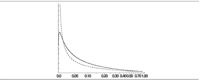
family of distributions (for details on the KL–dis-tance; see Agresti, 1990: p. 241). The resulting beta distribution has parameters a = 0.2512 and b = 1.1300. This beta distribution and the logit nor-mal distribution described in the previous para-graph are plotted in figure 1.

The observed and complete frequency distribu-tions are given in table 2. Note that while the observed frequency distributions are not identical, they are close enough to be virtually

indistinguish-able except with extremely large samples. The dis-crepancy in predictions of f₀ is substantial: based on n = 100, the predictions are 83 (for the logit– normal model) and 156 (for the beta model).

Ex a m ple 3

Expanding the term (1 – p)T–j _{in equation (1) by}

means of the binomial theorem, it is seen that the values (x) are linear combinations of the first T moments of distribution g(p), for x = 1,2,...,T. The same is true for

Let m_g(j) denote the jth moment of g(p). If we could construct a distribution h(p) with moments m_h(j) = cm_g(j), for some c g 1, and for j = 1,2,...,T, the observations in the previous paragraph, and the relation C_{(j) = (j)/(1 –}

_{(0)) lead to the}

conclusion that distributions g(p) and h(p) will induce the same values C_{(j), but different values}

for (0). Using subscripts g and h to distinguish the values of (0), we obtain the relation

(3) Thus these distinct distributions of heterogeneity will lead to the same sampling distributions for observed data, but different predictions for f₀, and consequently, for N.

If g(p) is the uniform distribution, m_g(j) = 1 / (j + 1). Consider the distribution function h(p) = 1/ 15 ( 114 – 4950 p + 79200 p2 _{– 600600 p}3 ₊

2522520 p4_{– 6306300 p}5 _{+ 9609600 p}6 _–

8751600 p7 _{+ 4375800 p}8 _{– 923780 p}9_).

This distribution is plotted along with the uni-form distribution in figure 2. Straightforward cal-culation shows that the moments of h(p) are m_h(j) = c / (j + 1), with c = 14 / 15, for j = 1,2,...,9. Thus for a study involving any number of sampling occasions up to T = 9, the data pro-duced with heterogeneity distribution h(p) will be Table 1. Cell probabilities for (x) and C_{(x) for complete and observed frequency distributions of}

Example 1.

Tabla 1. Probabilidades de cada celda para (x) y C_{(x) de las frecuencias de distribución completas}

y observadas del Ejemplo 1.

0 1 2 3 4 5 6

Unif (a,b) (x) .179048 .189616 .188057 .178371 .147685 .089382 .027840

C_{(x) – .230971 .229072 .217273 .179895 .108876 .033912}

3 pt. mixture (x) .133294 .200184 .198538 .188312 .155916 .094364 .029392

indistinguishable from data produced under a uniform distribution of heterogeneity. However, the predictions of f₀ will differ substantially. Since under the uniform distribution _g(0) = 1/(T + 1), we find from (3) and (2) that the prediction of f₀ based on the uniform distribution will be smaller than the prediction based on h(p) by a factor of 14 / (T + 15).

Some might dismiss this example on the grounds that they would never even consider fitting a distri-bution that looks like h(p); to this, I reply "That’s exactly my point!" If nature perversely selects h(p) as the distribution of heterogeneity, and we are (excusably) misled into assuming a uniform

distri-bution, our predictions of f₀ will be too small by a factor of 14 / (T + 15), and we’ll never know the difference.

Conc lusions a nd disc ussion

Population size N is not an identifiable parameter under model M_h, except under the imposition of untestable model assumptions. Thus estimation of population size, in the presence of individual het-erogeneity in detection is inevitably model based, much the same as the analysis of oft–reviled count survey data.

Table 2. Cell probabilities for (x) and C_{(x) for complete and observed frequency distributions of}

Example 2.

Tabla 2. Probabilidades de cada celda para (x) y C_{(x) de las frecuencias de distribución completas}

y observadas del Ejemplo 2.

0 1 2 3 4 5

Logit–normal (x) 0.454 0.208 0.126 0.090 0.070 0.052

C_{(x) – 0.381 0.231 0.165 0.128 0.095}

Beta (x) 0.609 0.149 0.090 0.065 0.050 0.037

C_{(x) – 0.381 0.231 0.166 0.127 0.095}

Fig. 1. Density functions used in Example 2. Dashed line represents beta distribution with parameters a = 0.2512 and b = 1.1300; solid line is distribution of p corresponding to logit(p) having a normal distribution with mean of –1.75 and standard deviation of 2.00. Note that x–axis has been distorted to accentuate the differences between the two densities.

Fig. 1. Funciones de densidad utilizadas en el Ejemplo 2. La línea discontinua representa la distribución beta con los parámetros a = 0,2512 y b = 1,300; la línea continua es la distribución de p correspondiente al logit(p) que presenta una distribución normal con una media de –1,75 y una desviación estándar de 2,00. Nótese que el eje x se ha distorsionado para acentuar las diferencias entre las dos densidades.

It is worth considering what the further impli-cations of this finding are, particularly for open population models. Some early indications (Link, 2003) are that while estimates of population sizes may be biased in a manner similar to that de-scribed here for closed population estimation, survival estimates may be less sensitive to het-erogeneity in detection rates. On the other hand, since capture–mark–recapture experiments es-sentially create "populations" of marked animals that are closed except to mortality, it is possible that time variation in detection rates might induce bias in survival estimates.

The problems presented here should come as no surprise. Indeed, without specific parametric models for the heterogeneity in p, we find our-selves in the unpleasant circumstances described in the classic paper of Kiefer & Wolfowitz (1956) which demonstrated, among other things, that maximum likelihood estimates of parameters of interest may be asymptotically biased, and badly so, if the number of nuisance parameters is al-lowed to increase without bound. This is pre-cisely the situation under model M_h, with indi-vidual detection probabilities in the role of nui-sance parameters.

Re fe re nc e s

Agresti, A., 1990. Categorical Data Analysis. New York, Wiley.

Burnham, K. P., 1972. Estimation of population size

in multiple capture–recapture studies when cap-ture probabilities vary among animals. Ph. D. Thesis, Oregon State Univ., Corvallis.

Burnham, K. P. & Overton, W. S., 1978. Estimation of the size of a closed population when capture probabilities vary among animals. Biometrika, 65: 625–633.

Coull, B. A. & Agresti, A., 1999. The use of mixed logit models to reflect heterogeneity in capture– recapture studies. Biometrics, 55: 294–301. Dorazio, R. M. & Royle, J. A., 2003. Mixture models

for estimating the size of a closed population when capture rates vary among individuals. Bio-metrics, 59: 351–364.

Huggins, R., 2001. A note on the difficulties associ-ated with the analysis of capture–recapture ex-periments with heterogeneous capture probabili-ties. Statistics and Probability Letters, 54: 147– 152.

Kiefer, J. & Wolfowitz, J., 1956. Consistency of the maximum likelihood estimator in the presence of infinitely many nuisance parameters. Annals of Mathematical Statistics, 27: 887–906.

Link, W. A., 2003. Nonidentifiability of population size from capture–recapture data with heteroge-neous detection probabilities. Biometrics, 59: 1125–1132.

Norris, J. L. & Pollock, K. H., 1996. Nonparametric MLE under two closed–capture modelswith het-erogeneity. Biometrics, 52: 639–649.

Pledger, S., 2000. Unified maximum likelihood estimates for closed capture–recapture models using mixtures. Biometrics, 56: 434–442. Fig. 2. Density functions used in Example 3. The first nine moments of the nonuniform density are precisely 14/15th’s the size of the corresponding moments of the uniform density.

Fig. 2. Funciones de densidad utilizadas en el Ejemplo 3. Los primeros nueve momentos de la densidad no uniforme equivalen precisamente a 14/15 del tamaño de los momentos homólogos de la densidad uniforme.

0.0 0.1 0.2 0.3 0.4 0.5 0.6 0.7 0.8 0.9 1.0 8