Simulation of the satellite radar altimeter sea ice thickness retrieval uncertainty

(1)

TCD

3, 513–559, 2009

Simulation of the satellite radar altimeter sea ice

R. T. Tonboe et al.

Title Page

Abstract Introduction

Conclusions References

Tables Figures

◭ ◮

Back Close

Full Screen / Esc

Printer-friendly Version

Interactive Discussion

The Cryosphere Discuss., 3, 513–559, 2009 www.the-cryosphere-discuss.net/3/513/2009/ © Author(s) 2009. This work is distributed under the Creative Commons Attribution 3.0 License.

The Cryosphere Discussions

The Cryosphere Discussionsis the access reviewed discussion forum ofThe Cryosphere

Simulation of the satellite radar altimeter

sea ice thickness retrieval uncertainty

R. T. Tonboe1, L. T. Pedersen1, and C. Haas2

1

Danish Meteorological Institute, Lyngbyvej 100, 2100 Copenhagen Ø, Denmark

2

University of Alberta, Edmonton, Alberta, Canada

Received: 23 June 2009 – Accepted: 7 July 2009 – Published: 21 July 2009

Correspondence to: R. T. Tonboe (rtt@dmi.dk)

(2)

TCD

3, 513–559, 2009

R. T. Tonboe et al.

Title Page

Tables Figures

◭ ◮

Back Close

Full Screen / Esc

Interactive Discussion Abstract

Although it is well known that radar waves penetrate into snow and sea ice, the exact mechanisms for radar-altimeter scattering and its link to the depth of the effective scat-tering surface from sea ice are still unknown. Previously proposed mechanisms linked the snow ice interface, i.e. the dominating scattering horizon, directly with the depth of

5

the effective scattering surface. However, simulations using a multilayer radar scatter-ing model show that the effective scattering surface is affected by snow-cover and ice properties. With the coming Cryosat-2 (planned launch 2009) satellite radar altimeter it is proposed that sea ice thickness can be derived by measuring its freeboard. In this study we evaluate the radar altimeter sea ice thickness retrieval uncertainty in terms of

10

floe buoyancy, radar penetration and ice type distribution using both a scattering model and “Archimedes’ principle”. The effect of the snow cover on the floe buoyancy and the radar penetration and on the ice cover spatial and temporal variability is assessed from field campaign measurements in the Arctic and Antarctic. In addition to these well known uncertainties we use high resolution RADARSAT SAR data to simulate errors

15

due to the variability of the effective scattering surface as a result of the sub-footprint spatial backscatter and elevation distribution sometimes called preferential sampling. In particular in areas where ridges represent a significant part of the ice volume (e.g. the Lincoln Sea) the simulated altimeter thickness estimate is lower than the real av-erage footprint thickness. This means that the errors are large, yet manageable if the

20

relevant quantities are known a priori. A discussion of the radar altimeter ice thickness retrieval uncertainties concludes the paper.

1 Introduction

Variation in sea ice thickness is a significant indicator for climate change (Wadhams, 1990; Rothrock et al., 2003), but its inter-annual, seasonal and spatial variability is

25

(3)

alter-TCD

3, 513–559, 2009

R. T. Tonboe et al.

Title Page

Tables Figures

◭ ◮

Back Close

Full Screen / Esc

native methods for monitoring sea ice thickness for climate monitoring such as satellite radar altimetry on the upcoming CryoSat-2, planned for launch in 2009 (Laxon et al., 2003; Wingham, 1999; Wingham et al., 2006), and laser altimetry using ICESat (Kwok et al., 2006; Kwok and Cunningham, 2008). The ice thickness is derived from al-timeters by multiplying the measured freeboard height by an e_ffective snow/ice density

5

factor (the K-factor). It is commonly assumed that radar altimeter signals operating at an electromagnetic frequency of about 13 GHz penetrate to the snow/ice interface. However, for pulse limited space-borne radar altimetry, backscatter modelling indicates that snow depth and density as well as snow and sea ice surface roughness influence the radar penetration into the snow and ice. As a result, the effective scattering surface

10

depth, which is the horizon where the freeboard is measured, can vary as a function of these snow and ice properties (Tonboe et al., 2006a). In addition, snow depth and density and ice density critically affect the floe buoyancy and the chances for estimat-ing sea ice thickness by measurestimat-ing its freeboard (Rothrock, 1986; Giles et al., 2007). The freeboard height is multiplied by the effective density to estimate the ice thickness

15

for a floe in hydrostatic equilibrium. Actually, the ice floe may not be in hydrostatic equilibrium on a point-by-point basis (Doronin and Kheisin, 1977), and this has conse-quences for the height measurements using radar as demonstrated in Sects. 4.5 and 4.6 below. However, on a floe to floe basis hydrostatic equilibrium logically is a valid assumption. Several ice thickness point measurements are needed to characterise the

20

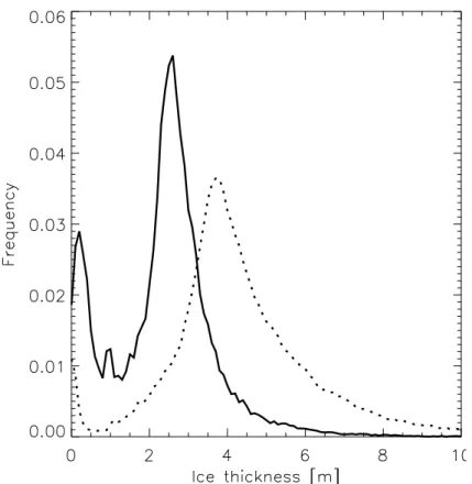
ice thickness distribution representative of a particular ice-covered region (Rothrock, 1986; Haas, 2003). The mode of the ice thickness distribution represents the dominat-ing thermodynamically grown thickness of level ice. However, the distribution has a tail towards thicker ice, i.e. deformed ice, and the average may be significantly different from the mode (Haas, 2003). Typical ice thickness distributions are shown in Fig. 1.

25

(4)

TCD

3, 513–559, 2009

R. T. Tonboe et al.

Title Page

Tables Figures

◭ ◮

Back Close

Full Screen / Esc

ice, as well as seasonally and regionally (Haas et al., 2006a; Wadhams et al., 1992). Tonboe et al. (2006b) pointed out that the parameters a_ffecting the sea ice freeboard and the radar penetration and ice type distribution are not mapped by any routine field campaign. The error-bars on the retrieved ice thickness estimates are needed when the data are assimilated into numerical models or when they are compared to other

5

ice thickness estimates such as those from laser altimeters, submarine sonars, drilling, and electromagnetic induction instruments. It is further important to identify the largest and most important error sources. Rothrock (1986) stated that the uncertainties in-volved in deriving the ice thickness from its freeboard were too large. However with the advent of modern space borne altimeters the issue has been revisited. Recent error

10

estimates of the ice thickness retrieval uncertainty for both laser (total error 0.76 m) and radar (total error 0.46 m) altimeters by Giles et al. (2007) included errors sources related to the floe buoyancy: i.e. the snow depth, freeboard estimation uncertainty, and the snow, ice and water density. The snow depth estimation error resulting in an ice thickness estimation error of 0.1 m in Giles et al. (2007) for the radar altimeter was the

15

most important of the error sources. The error due to radar penetration was assumed negligible in their budget, and the error due to systematic height and radar backscatter variability within the footprint was not considered. The importance of these two error sources is simulated here using snow and ice measurements and a radar scattering model.

20

The radar scattering model is a multilayer one-dimensional radiative transfer model where surface scattering is computed at horizontal interfaces (snow surface, icy layers and ice surface), as described in Tonboe et al. (2006a). Propagation speed, atten-uation and scattering are computed for each layer. The simulated echo delay due to freeboard variations and the time dependent backscatter intensity which is recorded

25

(5)

TCD

3, 513–559, 2009

R. T. Tonboe et al.

Title Page

Tables Figures

◭ ◮

Back Close

Full Screen / Esc

surface is the level detected by the 1/2-power time. On ice sheets, in regions where surface scattering dominates, the 1/2-power time “retracking” threshold gives a good representation of the mean surface elevation (Davis, 1997). We use the 1/2-power time since surface scattering mechanisms dominate sea ice backscatter. It is a robust measure of the distance to the effective scattering surface: simulations using seasonal

5

output from a thermodynamic model (snow cover parameters but not surface rough-ness or ice parameters) as input to the backscatter model show that the scattering surface follows the ice surface within about 5 cm during winter (Tonboe et al., 2006b). The model concept is different from single layer scattering models developed for ice sheet backscatter (e.g., Ridley and Partington, 1988) since surface scattering

domi-10

nates in sea ice i.e. scattering from the snow and ice surfaces and possibly from layers within the snow.

The specific aim of this study is to evaluate the radar altimeter sea ice thickness retrieval uncertainties in terms of both floe buoyancy and radar surface penetration combining a radar scattering model with “Archimedes’ principle” (Archimedes, 287–

15

212 BC). The primary sea ice thickness retrieval uncertainties are identified and dis-cussed in relation to the natural variability from field measurements. Further, the altime-ter footprint is not a point measurement, and thus the altimealtime-ter elevation measurement as a function of sub-footprint ice elevation and spatial backscatter intensity distribution is simulated using high resolution (50 m) SAR data.

20

2 Snow and ice properties

In situ data of snow and ice properties in the Central Arctic have always been sparse, but to overcome this problem there has been a long history of expeditions. From 1937 to 1991, the Soviet Union operated the series of North Pole drifting stations on multi-year ice floes (Frolov et al., 2006). In addition to the multi-year round drifting stations the

25

(6)

sum-TCD

3, 513–559, 2009

R. T. Tonboe et al.

Title Page

Tables Figures

◭ ◮

Back Close

Full Screen / Esc

mer melt, i.e. at the end of winter and therefore representing maximum thickness. The measurements were distributed geographically across the Arctic Ocean, but with higher frequency in the Eastern Arctic. The National Snow and Ice Data Center (NSIDC) re-ceived a subset of the Sever data also including data from the drifting stations (NSIDC, 2004). The data are described in Warren et al. (1999) and are used here to assess

5

the all-Arctic snow and ice variability. Furthermore, an extensive field programme di-rected towards ice thickness monitoring was carried out in the GREENICE project in the Fram Strait in April 2003 and in the Lincoln Sea in May 2004 (Haas et al., 2006b). These GREENICE activities were almost coincident and overlapping with the two SAR scenes used in this study; however, ice drift makes direct comparison difficult. The ice

10

thickness and snow thickness data obtained from both Fram Strait and the Lincoln Sea are representative of their respective regions during late winter and spring, and the ge-ographical distribution of these datasets is shown in Fig. 2. These measurements give the total ice thickness and the bulk density. However, layering and vertical variability of the snow cover properties is an inherent part of natural snow packs. The

layer-15

ing, in natural snow packs is formed by individual precipitation events where density is a function of wind speed and temperature during deposition. After deposition temper-ature gradient metamorphosis increases grain sizes and compaction and temporary melt may form icy layers. Three measured and detailed snow profiles from Antarctica are used to simulate the scattering in natural snow packs (Haas et al., 2008).

20

2.1 Use of SAR imagery

The standard mode RADARSAT SAR data classified into the four surface types (in Table 1) is used to prescribe realistic input ice type distributions. The SAR data classi-fication algorithm is based on fuzzy-logic principles. The classiclassi-fication is done by letting an experienced observer identify selected regions visually as belonging to one of the

25

(7)

TCD

3, 513–559, 2009

R. T. Tonboe et al.

Title Page

Tables Figures

◭ ◮

Back Close

Full Screen / Esc

Interactive Discussion 3 Modelling the depth of the effective scattering surface

The forward model uses a set of snow and ice microphysical parameters for each layer: temperature, layer thickness, density, correlation length ( a measure of the snow grain size or the ice inclusion size), interface roughness, salinity, and snow wetness to compute the effective scattering surface. The effective scattering surface is the level

5

detected by the 1/2-power time. The permittivity of dry snow is primarily a function of snow density, and the permittivity of sea ice is primarily a function of salinity and temperature. The permittivity of both materials is computed using the mixing formulae for rounded ice spheres (M ¨atzler, 1998):

εeff=

2ε1−ε2+2v(ε2−ε1)+ q

(2ε1−ε2+3v(ε2−ε1)) 2

+8ε1ε2

4 (1)

10

wherev is the fraction of volume occupied by inclusions,ε1is the host permittivity of the material surrounding the inclusions andε₂is the permittivity of the inclusions. For snowε1is the permittivity of air (εair=1), and for saline ice,ε1is the permittivity of pure ice given in M ¨atzler et al. (2006). For snow the inclusions are pure ice, and for saline first-year ice the inclusions are brine pockets. The permittivity and also the volume of

15

brine are given in Ulaby et al. (1986). For multiyear ice the host material is saline ice and the inclusions are air bubbles.

When the snow reaches the melting point the absorption by liquid water increases the dielectric loss dramatically. The permittivity of wet snow is given in Ulaby et al. (1986). The same formulation is used for saline snow since the permittivity of

20

brine and fresh liquid water is nearly the same at 13 GHz. The permittivity of snow and ice using the equations above is given in Tables 2–5.

(8)

TCD

3, 513–559, 2009

R. T. Tonboe et al.

Title Page Abstract Introduction Conclusions References Tables Figures ◭ ◮ ◭ ◮ Back Close

Full Screen / Esc

reflection coefficient|R(0)|and the flat-patch areaF (Fetterer et al., 1992), i.e.

σsurf=0.9F|R(0)|2 H

uτ , (2)

whereH is the satellite height, u the pulse propagation speed (speed of light in air, snow and ice, respectively) andτ the pulse length. F is the flat-patch area, which is inversely related to roughness (i.e., smooth surface have highF). This model assumes

5

that the signal is dominated by reflection processes from relatively small plane areas (flat-patches) normal to the incident signal within the footprint. In the review of different surface scattering models in Fetterer et al. (1992) the approach in Eq. (2) is believed to be “more realistic” than other models. The geometrical optics model, which is an alternative to Eq. (2), makes very similar predictions. The basic concept for all

sur-10

face scattering models is that the backscatter is a function of reflection coefficient and surface roughness; i.e., when the surface is smooth the backscatter is high, and when the surface is rough then the backscatter is smaller. All models described in Fetterer et al. (1992), including Eq. (2), make that prediction.

The improved Born approximation, suitable for microwave scattering in a dense

15

medium such as snow, is used to compute the volume scattering coefficient (M ¨atzler, 1998; M ¨atzler and Wiesmann, 1999). Volume scattering is scattering from particles or inclusions within layers, i.e. snow grains within the snow layers, and air bubbles and brine pockets within the ice layers.

The improved Born approximation for spherical inclusions is (M ¨atzler, 1998)

20

σvol∼₌ 3p

3 eck

4

32 v(1−v)

(ε₂−ε₁)(2ε_e_ff+ε₁) 2εeff+ε2

2 , (3)

wherepec is the correlation length,k the wavenumber,νthe volume fraction of scat-terers, and ε1,ε2, εeff are the permittivity of the background, the scatterers, and the layer, respectively. Volume scattering is an important backscatter mechanism for scat-terometers operating at 13 GHz and about 50◦incidence such as QuikScat SeaWinds.

(9)

TCD

3, 513–559, 2009

R. T. Tonboe et al.

Title Page

Tables Figures

◭ ◮

Back Close

Full Screen / Esc

However, the total altimeter backscatter is dominated by surface (or interface) scatter-ing, and in our altimeter simulations volume scattering is insignificant as a backscatter source. This is in agreement with laboratory experiments showing that at nadir inci-dence, volume scattering is insignificant as a backscatter source for snow-covered sea ice (Beaven et al., 1995). Though volume scattering is not a backscatter source, it

5

does increase extinction and to some extent the distribution of backscatter between the snow and the ice surface. This distribution and the snow depth do affect the depth of the e_ffective scattering surface (Tonboe et al., 2006a).

No specific correction is applied for antenna gain or pulse modulation in the char-acterisation of the emitted pulse. We use a geometric description of the footprint area

10

in each layer i as a function of time t from Chelton et al. (2001) for a pulse-limited altimeter,

A_i(t)= πuitH

1+H/Re

−πui(t−τ)H 1+H/Re

, (4)

where the second term is 0 whent<τ. Re is Earth’s radius (6371 km),ui is the speed of light in the layer andH is the satellite height (800 km).

15

The waveform model integrates the time-dependent backscatter from each scattering horizon. The pulse propagation speed, signal extinction and backscatter are computed as the pulse penetrates the profile, and each individual contribution is summed with appropriate time delay. The backscattered energy, E, measured at the satellite for each model time-step (1×10−11s), is the sum of the footprint area,Ai, multiplied by the

20

layer backscatter coefficient,σi, i.e.

E_t= n X

i=1

A_iσ_i (5)

(10)

TCD

3, 513–559, 2009

R. T. Tonboe et al.

Title Page

Tables Figures

◭ ◮

Back Close

Full Screen / Esc

the radiative transfer approach, i.e.

σtotal=

σ_isurf+T_i2σ_ivol n Y

i=1 1

L2

i−1

T_i2₋₁. (6)

Lis the loss and T the transmission coefficient whereL0=T0=1 for the first layer and

σvolis the negligible volume backscatter coe_fficient.

4 Simulation results

5

4.1 Combining the depth of the effective scattering surface with ice buoyancy

Since both the height of the scattering surface and the floe buoyancy are affected by snow depth and snow density, the scattering model is used together with “Archimedes’ principle” to compute the sensitivity of both simultaneously. The surface roughness affects the height of the scattering surface and the ice density affects primarily the floe

10

buoyancy. Snow measurements are input to the model in order to translate the natural snow variability to simulated range variability. The measurements are from the Russian Sever project (NSIDC, 2004) and the EU GREENICE project (Haas et al., 2006b). The locations of the measurements are shown in Fig. 2.

Natural snow and ice profiles are more complicated than what is indicated by

Ta-15

ble 2. Layering is an inherent part of natural snow packs (Wiesmann et al., 1998), and melt-water and brine may be included in the snow. Also, snow grain sizes and sea ice inclusion size may deviate significantly from the values given in Table 2. In order to illustrate the sensitivity to liquid water, icy layers, and snow grain sizes we use a selection of measured profiles from the Weddell Sea (Haas et al., 2008).

20

(11)

TCD

3, 513–559, 2009

R. T. Tonboe et al.

Title Page

Tables Figures

◭ ◮

Back Close

Full Screen / Esc

Table 1 are used as a look-up table in the simulations. The waveform model is using a 10−11s time-step.

4.2 1-D sensitivity study

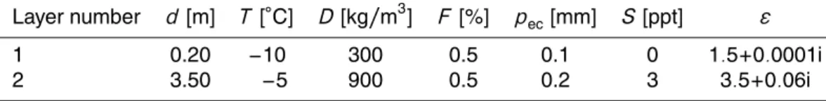
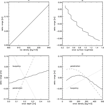
Table 2 is a reference for the sensitivity simulation study shown in Fig. 3. Each param-eter (ice density, ice surface roughness, snow density and snow depth) is evaluated

5

separately, and both buoyancy and radar penetration effects are included. The profile in Table 2 has a snow freeboard of 0.6 m (water density is 1035 kg/m3). The range over which the parameters are varied is assumed to provide realistic upper and lower bounds. The ranges of surface roughness and ice density values are discussed in Sect. 4.3, and the sensitivity to snow depth and snow density using measurements as

10

input is shown in Sect. 4.4.

4.3 The sea ice density and the surface roughness

Density of multiyear ice varies between 720 and 910 kg/m3, and of first-year ice be-tween 900 and 940 kg/m3, and densities of the submerged part varies between 900 and 940 kg/m3for both ice types. Typical variability of the ice density is between 5 and

15

10 kg/m3(Wadhams et al., 1992). Sea ice density is related to its salinity, temperature and air bubble volume (Timco and Frederking, 1996; Cox and Weeks, 1983). Increas-ing ice density makes the ice floe sink thus extendIncreas-ing the range to the snow surface, as well as the apparent ice surface and the scattering surface (Fig. 3a). Decreasing ice density raises the snow, ice and scattering surface thus shortening range.

20

Surface roughness is a central model parameter (Dierking et al., 1997). Using Eq. (2) Fetterer et al. (1992) estimates that for realistic backscatter values between 20 and 40 dB the flat-patch-area is between 0.2% and 16%. Some ice types such as multiyear ice (10–20 dB) and deformed ice (10 dB) have even lower backscatter values. Following the reasoning from Fetterer et al. (1992) this means that the flat-patch-area could be

25

(12)

TCD

3, 513–559, 2009

R. T. Tonboe et al.

Title Page

Tables Figures

◭ ◮

Back Close

Full Screen / Esc

does not affect floe buoyancy but instead the vertical distribution of backscattering between the snow and ice surface and thus the e_ffective scattering surface. There is more backscatter from a smoother snow surface (see Eq. 2), and thus the effective scattering surface is lifted leading to shortening the range. It is not known how the snow-ice interface roughness varies in time and space. Therefore it is di_fficult to assess

5

the importance of this parameter for the effective scattering surface. However, surface roughness is the primary factor affecting the sub-footprint spatial backscatter variability which will be discussed in Sect. 4.5.

4.4 Effect of variation of snow depth and density

The climatology of snow cover on sea ice measured at Russian drift stations is

de-10

scribed in Warren et al. (1999): the mean Arctic Ocean snow depth increases during the cold season from September to June from zero to about 34 cm. The maximum snow depth (46 cm in June) is in the Lincoln Sea and there are local minima north of Siberia and Alaska. The mean snow density increases from 250 kg/m3 in September to 320 kg/m3 in May. Regional snow density variations are small (about 25 kg/m3 in

15

May). Maximum snow thickness on 17 mass balance buoys distributed in the Arctic Ocean for the years 1993-2005 (Richter-Menge et al., 2006) averaged 33.6 cm (stan-dard deviation 12.6 cm). The deepest snow was 60 cm. Spatially, the snow depth variability is large on sea ice (Warren et al., 1999).

Deeper snow on sea ice (Fig. 3c) suppresses the ice surface and raises the snow

20

surface. The scattering surface is not suppressed as much as the ice surface. The result is a range extension for deeper snow. The snow depth distributions from the GREENICE experiments and the Sever project are shown in Fig. 4. The snow depth records are input to the model replacing the snow thickness value in Table 2. In the computations this comprises both radar penetration and profile buoyancy for the range

25

(13)

TCD

3, 513–559, 2009

R. T. Tonboe et al.

Title Page

Tables Figures

◭ ◮

Back Close

Full Screen / Esc

the regional GREENICE datasets are small. The range variability using the measured data input is about 6 cm.

Snow density affects the buoyancy (dashed line in Fig. 3d) as well as the reflection coefficient at both the snow and ice surface, hence also the distribution of backscatter (see Eq. 2). The scattering surface is therefore lifted for greater snow density (the

5

dash-dot line in Fig. 3d). The result is a slightly shorter range for densities above 300 kg/m3. Measured snow densities from the Sever project are then used as input with the other values from Table 2 in the model, computing both radar penetration and profile buoyancy. The range of measured snow densities is shown in Fig. 6 with a median of 330 kg/m3and values between 170 kg/m3and 460 kg/m3. The simulated

10

range variability is shown in Fig. 7 for two di_fferent snow thickness values: 0.2 m, as in Table 2, and 0.3 m. The simulated range variability using the measured data input is about 6 to 8 cm.

4.5 Effect of two ice types within the footprint

High backscatter from limited smooth areas within the footprint can dominate the total

15

altimeter backscatter coefficient as well the height of the effective scattering surface because the backscatter is nonlinear function of the surface roughness (Fetterer et al., 1992).

In a simulation experiment, shown in Fig. 8, multiyear ice, 3 m thick, is mixed with new ice, 0.1 m thick (see Table 1). The footprint is totally ice covered with these two

20

types. It is assumed that when only one ice type covers the entire footprint its eleva-tion and thickness can be estimated perfectly with the altimeter 1/2-power time. The backscatter coefficient for the multiyear ice is 15 dB and for the new ice is 10 times higher: 25 dB (Fetterer et al., 1992). For a 99% multiyear ice-cover with 1% new ice the simulated altimeter ice thickness is underestimated by 26 cm compared to the

av-25

(14)

TCD

3, 513–559, 2009

R. T. Tonboe et al.

Title Page

Tables Figures

◭ ◮

Back Close

Full Screen / Esc

Interactive Discussion 4.6 Simulation of the sub-footprint ice type distribution using SAR data

SAR scenes were analysed in the two different ice regimes in the Fram Strait and in the Lincoln Sea (Gill and Tonboe, 2006). A map is shown in Fig. 2. Fig. 9a and b are typical scenes for each of the regions. In situ observations during the GREENICE field activities within the frame of both scenes in 2003 and 2004 at the time of acquisition

5

indicate that the classification is realistic. Figure 9a shows the distribution of ice types in the Lincoln Sea in May 2004. The ice-cover is complete and dominated by multiyear ice (84.4%) with fractions of new-ice (1.3%), first-year ice (2.9%) and pressure ridges (11.4%). Figure 9b shows the distribution of ice types in Fram Strait in April 2003. Also here the ice-cover is complete and dominated by multiyear ice (63.9%) with fractions

10

of new-ice (1.5%), first-year ice (33.9%) and pressure ridges (0.7%).

The SAR images are divided into 250 m×7000 m altimeter footprints (this size corre-sponds to CryoSat’s sea ice mode), and these are then used as input to the waveform model. Each of the four ice types is assigned a fixed backscatter coefficient, using val-ues from Fetterer et al. (1992) given in Table 1. The ice thickness for each of the four

15

types roughly corresponds to the modes of the ice thickness distribution measured within the 2003 SAR frame (Haas et al., 2006b). The ice thickness distribution with modes of around 0.1 m, 1 m and 3 m is shown in Fig. 1.

The backscatter and ice thickness look-up-table values are summarised in Table 1. It is assumed that when only one ice type covers the entire footprint its elevation and

20

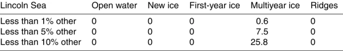
thickness can be estimated perfectly with the altimeter as in the example in Sect. 4.4 (the “retracking” threshold is tuned to the ice surface and its density is known). Fewer than 0.5% of the “footprints” in the SAR scenes are covered by just one ice type. Table 7 and 8 show the percentage of footprints where only a small fraction (1%, 5% and 10%) of the footprint is covered by other ice types. In the Fram Strait (Table 8) there are

25

(15)

TCD

3, 513–559, 2009

R. T. Tonboe et al.

Title Page

Tables Figures

◭ ◮

Back Close

Full Screen / Esc

within each footprint, and the simulated ice thickness is estimated using the waveform model, Table 1, and the footprint ice type distribution in the SAR image. The simulated thickness distributions from each scene are shown in Figs. 10 and 11. The effects of snow are not included. The measured ice thickness distributions are shown from both the Lincoln Sea and the Fram Strait in Fig. 1.

5

Figure 12a and b shows that in the Lincoln Sea, where the fraction of ridges largely determines the average footprint ice thickness in our simulation, the simulated altimeter ice thickness is much less than the true ice thickness in areas with ridges.

In the Fram Strait, shown in Fig. 12c and d, the simulated altimeter ice thickness is lower than the average footprint thickness in particular areas with mixed ice types, i.e.

10

multiyear ice, first-year ice and new-ice.

It is possible that sub-SAR-resolution surface roughness patterns on multiyear ice can have similar effect on the elevation estimate. While melt ponds typically have smooth surfaces, hummocks have rough surfaces (Onstott, 1992). Hummocks have higher freeboard than refrozen melt ponds and though this pattern is not resolvable in

15

our SAR data it represents the same height and backscatter pattern as thin and thick ice does. Therefore a multiyear ice floe with deeper melt ponds may appear thinner than a floe with not so deep melt ponds due to the preferential sampling of the melt ponds.

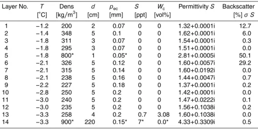
4.7 Measured snow and ice profiles from the Weddell Sea

20

Snow depths on Antarctic sea ice are large compared to the Arctic, and temporary melt may occur even in winter, which means that the snow packs can have large vertical diversity. However, liquid water and layering in the snow-pack are also relevant for Arctic sea ice, especially during spring. Three measured snow profiles in the Weddell Sea were selected due to their different backscatter intensity in QuikScat SeaWinds

25

(16)

TCD

3, 513–559, 2009

R. T. Tonboe et al.

Title Page

Tables Figures

◭ ◮

Back Close

Full Screen / Esc

three profiles, respectively. The snow correlation length (pec) is converted from snow grain size and snow type measurements according to Fig. 2, in Wiesmann et al. (1998, p. 275). The surface roughness was not measured but has been set constant to 0.5% for all layer surfaces. Other estimated parameters in the profiles are marked with (*). In particular the icy layers have been assigned the density 800 kg/m3and the ice density

5

is set to 900 kg/m3. The permittivity and the partial backscatter from each layer are computed using the model. As stated in Eq. (2) the backscatter is a function of surface roughness and the reflection coe_fficient. Roughness is constant here and the snow reflection coefficient is primarily a function of snow density.

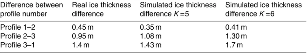
Profile 1 in Table 3 has 0.21 m snow on top of 0.8 m ice. The upper snow layers

10

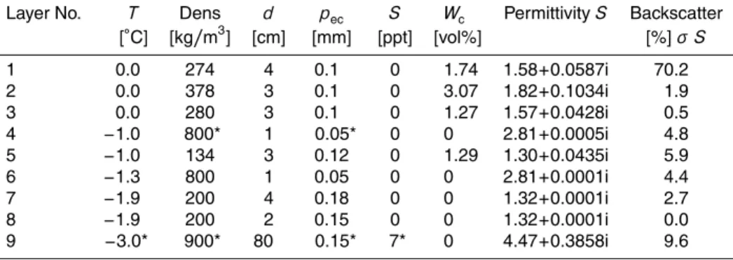
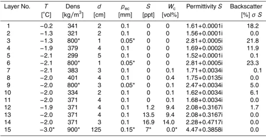
are wet. Profile 2 in Table 4 has 0.42 m snow on 1.25 m ice. Profile 3 in Table 5 has 0.53 m snow on 2.2 m ice. The penetration depth at 13 GHz in all three profiles is less than the snow depth. The penetration depth, where the unit power beneath the surface has decreased to 1/e (0.37), was computed using the radar model. Penetration depth is 0.06 m in profile 1, 0.33 m in profile 2, and 0.46 m in profile 3. The absolute

15

freeboard was not measured in situ but the estimated ice thickness differences are compared in Table 6. Two effective density factors (K=5 andK=6) were tested. For the given density profiles and radar penetration K=5 gives the smallest differences. It is noted that the three thickness categories are distinguishable, i.e. the range from the satellite to the effective scattering surface given by the 1/2-power time is longer for

20

profile 1 than for profile 2 and 3. The simulated waveform for each profile is shown in Fig. 13. All three profiles have icy layers and liquid water in the snow pack and most of the simulated backscatter from each layer comes from the top of the snow pack. In particular, icy layers and attenuation by liquid water are important for the vertical distribution of backscatter.

(17)

TCD

3, 513–559, 2009

R. T. Tonboe et al.

Title Page

Tables Figures

◭ ◮

Back Close

Full Screen / Esc

5 Discussion and conclusions

It is important to identify the most significant error sources so that these can be mon-itored and the ice thickness estimates corrected accordingly. Even though there are some di_fferences in recent estimates of the variability of the snow and ice parameters affecting the floe buoyancy and the ice thickness retrieval uncertainty estimates, it is

5

clear that four parameters are important: snow depth, ice density, freeboard estima-tion error and snow density (Giles et al., 2007; Kwok and Cunningham, 2008). The simulations in this study show that the radar penetration variability and the preferential sampling error are as important error sources as those affecting the floe buoyancy.

5.1 Buoyancy and penetration

10

Our simulations including both the radar penetration and the floe buoyancy show that when snow depth and snow density increase and the ice freeboard (snow/ice inter-face) is lowered, then the effective scattering surface is raised compared to the refer-ence case (Fig. 3c and d). This means that the errors due to buoyancy may partly be compensated by radar penetration and the total error is therefore moderate.

Neverthe-15

less, for these two snow parameters it will be important to correct for both buoyancy and radar penetration. Further, using snow and ice climatology for correcting the ice thickness estimate may, on average, reduce the total error; it introduces, however, an ice thickness estimate bias for any snow cover or ice density deviating from the cli-matology. Therefore, using climatology it will be difficult to distinguish climate or inter

20

annual snow thickness and ice density variability on the one hand from ice thickness anomalies on the other hand.

5.2 Spatial variability and preferential sampling

Figure 8 (average thickness) shows that the high backscatter magnitude from the thinnest ice within the footprint largely determines the elevation of the effective

(18)

TCD

3, 513–559, 2009

R. T. Tonboe et al.

Title Page

Tables Figures

◭ ◮

Back Close

Full Screen / Esc

tering surface. Because of this preferential sampling of the thinner ice types it will be important to measure just one ice type at a time. In fact it may be possible to iden-tify echoes from surfaces which are a mix of ice types (Giles et al., 2007). However, nearly all footprints in the two SAR scenes are a mix of different ice types. Because of the limited spatial extent of both new ice and ridges it is not possible to find footprints

5

which are more than 50% covered by these two types within the two SAR scenes. This may be acceptable for sampling new ice because of its high backscatter, but the ridge freeboard will be significantly underestimated. A significant part of the ice volume is found in ridges (Haas, 2003). In the SAR image from the Lincoln Sea ridges occupy 11% of the ice-covered area, which is 31% of the volume assuming thickness values

10

from Table 1. The simulations using the SAR data show that although the ridges are significant for the average ice thickness, they have low backscatter intensity and are therefore underestimated in the simulated altimeter thickness estimate by the prefer-ential sampling of thinner ice. In the Fram Strait, primarily a mixture between level multiyear ice and first-year ice, the average footprint thickness distribution is a mirror

15

image of the simulated altimeter thickness estimate. It thus seems from the simulations that this error can be minimized in regions where one ice type dominates and where ridges are insignificant for the ice volume.

5.3 Snow and ice parameters relevant for the ice thickness retrieval uncertainty

Clearly, systematic monitoring is needed for key parameters such as for snow

thick-20

ness and density, ice density, surface roughness and ice type distribution, in order to distinguish altimeter ice thickness anomalies from the noise introduced by these other parameters.

The sub-footprint spatial variability of backscatter intensity and surface elevation cre-ates a bias towards the smooth parts of the ice, i.e., new and first-year ice, along with

25

(19)

TCD

3, 513–559, 2009

R. T. Tonboe et al.

Title Page

Tables Figures

◭ ◮

Back Close

Full Screen / Esc

volume.

Few studies have investigated the sea ice density variability (Timco and Frederk-ing, 1996). Typical ice density variability of 5 to 10 kg/m3 is mentioned in Wadhams et al. (1992) while Timco and Frederking (1996) state that the density can vary between 900 and 940 kg/m3. The density varies with salinity, temperature and gas volume, i.e.

5

ice type, which indicates that there can be a systematic variation from region to re-gion. Ice density variability of 5, 10 or 20 kg/m3 results in errors in the estimated ice thickness of 0.17 m, 0.34 m or 0.68 m, respectively.

The snow cover affects the buoyancy and the effective scattering surface depth. Us-ing snow cover measurements as input to the model, the range variability is about

10

6 cm for both snow depth and density. Multiplying by an effective density and radar penetration factor for the snow and ice system (K-factor) of 5 this gives a 0.3 m ice thickness variability for both parameters. The effective scattering surface depth is thus affected by the snow and ice surface roughness. However, we were not able to find any measurements of surface roughness to account for both ice and snow surface.

15

The simulations for a range of values indicate that the range variability is about 8 cm, giving an ice thickness error of 0.4 m withK=5.

Today these parameters are not all monitored systematically. A systematic effort is needed to evaluate the changes in the Arctic Ocean sea ice observed by current and planned satellite altimeters.

20

Acknowledgements. This work was supported by the EU GREENICE (EVK2-2001-00280) and

the EU DAMOCLES (018509) projects.

References

Archimedes. On floating bodies I, in: The Works of Archimedes, edited by: Heath, T. L., Dover publications, Inc., New York, 1897.

25

(20)

TCD

3, 513–559, 2009

R. T. Tonboe et al.

Full Screen / Esc

Perovich, D. K., Fung, A. K., and Tjuatja, S.: Laboratory measurements of radar backscatter from bare and snow-covered saline ice sheets, Int. J. Remote Sens., 16, 851–876, 1995. Cox, G. F. N. and Weeks, W. F.: Equations for detirmining the gas and brine volumes in sea ice

samples, J. Glaciol., 29, 306–316, 1983.

Davis, C.: A robust threshold retracking algorithm for measuring ice sheet surface elevation

5

change from satellite radar altimeters, IEEE Trans. Geosci. Remote Sens., 35, 974–979, 1997.

Dierking, W., Carlstr ¨om, A., and Ulander, L. M. H.: The effect of inhomogeneous roughness on radar backscattering from slightly deformed sea ice, IEEE T. Geosci. Remote, 35, 147–159, 1997.

10

Doronin, Y. P. and Kheisin, D. E.: Sea Ice, Amerind Publ. Co. Pvt. Ltd., New Delhi, 1977. Fetterer, F. M., Drinkwater, M. R., Jezek, K. C., Laxon, S. W. C., Onstott, R. G., and

Ulan-der, L. M. H.: Sea ice altimetry, in: Microwave Remote Sensing of Sea Ice, Geophysical Monograph 68, edited by: Carsey, F. D., American Geophysical Union, Washington DC, pp. 111–135, 1992.

15

Frolov, I. E., Gudkovich, Z. M., Radionov, V. F., Shirochkov, A. V., and Timokhov, L. A.: The Arctic Basin – Results from the Russian Drifting Stations, Springer Praxis Books, 2006. Giles, K. A., Laxon, S. W., Wingham, D. J., Wallis, D. W., Krabill, W. B., Leuschen, C. J.,

McAdoo, D., Manizade, S. S., and Raney, R. K.: Combined airborne laser and radar altime-ter measurements over the Fram Strait in May 2002, Remote Sens. Environ., 111, 182–194,

20

2007.

Gill, R. S., Tonboe, R. T.: Classification of GreenICE SAR data using fuzzy screening method. Arctic Sea Ice Thickness: Past, Present and Future, edited by: Wadhams and Amanatidis, Climate Change and Natural Hazards Series 10, EUR 22416, 2006.

Haas, C.: Dynamics versus thermodynamics: The sea ice thickness distribution, in: Sea Ice,

25

edited by: Thomas, D. N. and Dieckmann, G. S., Blackwell, 2003.

Haas, C., Goebell, S., Hendricks, S., Martin, T., Pfaffling, A., and von Saldern, C.: Airborne electromagnetic measurements of sea ice thickness: Methods and applications. Arctic Sea Ice Thickness: Past, Present and Future, edited by: Wadhams and Amanatidis, Climate Change and Natural Hazards Series 10, EUR 22416, 2006a.

30

(21)

TCD

3, 513–559, 2009

R. T. Tonboe et al.

Full Screen / Esc

Haas, C., Hendricks, S., and Doble, M.: Comparison of the sea ice thickness distribution in the Lincoln Sea and adjacent Arctic Ocean in 2004 and 2005, Ann. Glaciol., 44, 247–252, 2006b.

Kwok, R. and Cunningham, G. F.: ICESat over Arctic sea ice: Estimation of snow depth and ice thickness, J. Geophys, Res., 113, C08010, doi:10.1029/2008JC004753, 2008.

5

Kwok, R., Cunningham, G. F., Zwally, H. J., and Yi, D.: ICEsat over Arctic sea ice: Interpretation of altimetric and reflectivity profiles, J. Geophys. Res., 111, C06006, doi:10.1029/2005JC003175, 2006.

Laxon, S., Peacock, N., and Smith, D.: High interannual variability of sea ice thickness in the Arctic region, Nature, 425, 947–949, 2003.

10

M ¨atzler, C.: Improved Born approximation for scattering of radiation in a granular medium, J. Appl. Phys., 83, 6111–6117, 1998.

M ¨atzler, C. and Wiesmann, A.: Extension of the microwave emission model of layered snow-packs to coarse grained snow, Remote Sens. Environ., 70, 317–325, 1999.

M ¨atzler, C., Rosenkranz, P. W., Battaglia, A., and Wigneron, J. P.: Thermal Microwave Radiation

15

– Applications for Remote Sensing, IET Electromagnetic Waves Series 52, London, UK, 2006.

McLaren, A. S., Walsh, J. E., Bourke, R. H., Weaver, R. L., and Wittmann, W.: Variability in the sea-ice thickness over the North Pole from 1977 to 1990, Nature, 358, 224–226, 1992. National Snow and Ice Data Center. Morphometric characteristics of ice and snow in the Arctic

20

Basin: aircraft landing observations from the Former Soviet Union, 1928–1989. Compiled by Romanov, I. P., Boulder, CO: National Snow and Ice Data Center. Digital media, 2004. Onstott, R. G.: SAR and scatterometer signatures of sea ice, in: Microwave Remote Sensing of

Sea Ice, Geophysical Monograph 68, edited by: Carsey, F. D., American Geophysical Union, Washington DC, 73–104, 1992.

25

Richter-Menge, J. A., Perovich, D. K., Geiger, C., Elder, B. C., and Claffey, K.: Ice mass bal-ance buoy: An instrument to measure and attribute changes in ice thickness. Arctic Sea Ice Thickness: Past, Present and Future, edited by: Wadhams and Amanatidis, Climate Change and Natural Hazards Series 10, EUR 22416, 2006.

Ridley, J. K. and Partington, K. C.: A model of satellite radar altimeter return from ice sheets,

30

Int. J. Remote Sens., 9, 601–624, 1988.

(22)

TCD

3, 513–559, 2009

R. T. Tonboe et al.

Title Page

Tables Figures

◭ ◮

Back Close

Full Screen / Esc

551–575, 1986.

Rothrock, D. A., Zhang, J., and Yu, Y.: The arctic ice thickness anomaly of the 1990s: A consistent view from observations and models, J. Geophys. Res., 108, 3083, doi:10.1029/2001JC001208, 2003.

Timco, G. W. and Frederking, R. M. W.: A review of sea ice density, Cold Reg. Sci. Technol.,

5

24, 1–6, 1996.

Tonboe, R. T., Andersen, S., Gill, R. S., and Toudal Pedersen, L.: The simulated seasonal variability of the Ku-band radar altimeter effective scattering surface depth in sea ice. Arctic Sea Ice Thickness: Past, Present and Future, edited by: Wadhams and Amanatidis, Climate Change and Natural Hazards Series 10, EUR 22416, 2006b.

10

Tonboe, R., Andersen, S., and Toudal Pedersen, L.: Simulation of the Ku-band radar altimeter sea ice effective scattering surface, IEEE Geosci. Remote S., 3, 237–240, 2006a.

Ulaby, F. T., Moore, R. K., and Fung, A. K.: Microwave Remote Sensing, from Theory to Appli-cations, vol. 3, Artech House, Dedham MA, 1986.

Wadhams, P.: Evidence for thinning of the Arctic ice cover north of Greenland, Nature, 345,

15

795–797, 1990.

Wadhams, P., Tucker III, W. B., Krabill, W. B., Swift, R. N., Comiso, J. C., and Davis, N. R.: Relationship between sea ice freeboard and draft in the Arctic basin and implications for sea ice monitoring, J. Geophys. Res., 97, 20325–20334, 1992.

Warren, S. G., Rigor, I. G., Untersteiner, N., Radionov, V. F., Bryazgin, N. N., Aleksandrov, Y. I.,

20

and Colony, R.: Snow Depth on Arctic Sea Ice, J. Climate, 12, 1814–1829, 1999.

Wiesmann, A., M ¨atzler, C., and Weise, T.: Radiometric and structural measurements of snow samples, Radio Sci., 33, 273–289, 1998.

Wingham, D. J., Francis, C. R., Baker, S.: CryoSat: A mission to determine the fluctuations in Earth’s land and marine fields, Adv. Space Res., 37, 841–871, 2006.

25

(23)

TCD

3, 513–559, 2009

R. T. Tonboe et al.

Title Page

Tables Figures

◭ ◮

Back Close

Full Screen / Esc

Table 1. Elevation and backscatter values from Fetterer et al. (1992), the values are used

as a look-up-table for the four ice types identified in the SAR scenes: new ice, first-year ice, multiyear ice and ridges.

New ice First-year ice Multiyear ice Ridges

(24)

TCD

3, 513–559, 2009

R. T. Tonboe et al.

Title Page

Tables Figures

◭ ◮

Back Close

Full Screen / Esc

Table 2. The physical properties of the reference profile. d is the layer thickness, T is the

temperature,D is the density,F is the flat-patch area (inversely related to roughness),p_ec is the correlation length,S is the salinity,εis the permittivity computed with the model.

Layer number d[m] T [◦C] D[kg/m3] F [%] pec[mm] S[ppt] ε

(25)

TCD

3, 513–559, 2009

R. T. Tonboe et al.

Title Page

Tables Figures

◭ ◮

Back Close

Full Screen / Esc

Table 3.Profile 1. The snow cover depth is 0.21 m and the ice thickness is 0.8 m. The numbers

marked with * are not measured. The total backscatter coefficient from profile 1 is 18.9 dB and the partial backscatter from each layer is given in the right column in percent. Columns marked with S are simulated with the model using the measured input. Layer 4 is an icy layer.

Layer No. T Dens d p_ec S W_c PermittivityS Backscatter

[◦C] [kg/m3] [cm] [mm] [ppt] [vol%] [%]σ S

1 0.0 274 4 0.1 0 1.74 1.58+0.0587i 70.2

2 0.0 378 3 0.1 0 3.07 1.82+0.1034i 1.9

3 0.0 280 3 0.1 0 1.27 1.57₊0.0428i 0.5

4 −1.0 800* 1 0.05* 0 0 2.81+0.0005i 4.8

5 −1.0 134 3 0.12 0 1.29 1.30+0.0435i 5.9

6 −1.3 800 1 0.05 0 0 2.81+0.0001i 4.4

7 −1.9 200 4 0.18 0 0 1.32₊0.0001i 2.7

8 −1.9 200 2 0.15 0 0 1.32+0.0001i 0.0

(26)

TCD

3, 513–559, 2009

R. T. Tonboe et al.

Title Page

Tables Figures

◭ ◮

Back Close

Full Screen / Esc

Table 4. Profile 2. The snow cover depth is 0.42 m and the ice thickness is 1.25 m. The

numbers marked with * are not measured. The total backscatter coefficient from profile 2 is 25.1 dB and the partial backscatter from each layer is given in the right column in percent. Columns marked with S are simulated with the model using the measured input. Layers 3, 6, and 9 are icy layers.

1 −0.2 341 2 0.1 0 0 1.61+0.0001i 18.2

2 −1.3 321 2 0.1 0 0 1.56₊0.0001i 0.0

3 −1.3 800* 1 0.05* 0 0 2.81+0.0005i 21.8

4 −1.9 379 4 0.1 0 0 1.69+0.0002i 11.9

5 −2.1 299 5 0.1 0 0 1.52+0.0001i 0.1

6 −2.1 800* 1 0.05* 0 0 2.81+0.0005i 23.3

7 −2.1 383 3 0.1 0 0.1 1.71+0.0034i 0.1

8 −2.0 401 4 0.1 0 0.4 1.75+0.0135i 0.0

9 −2.0 800* 3 0.05* 0 0.1 2.47+0.0034i 5.0

10 −2.0 334 2 0.1 0 0.1 1.62+0.0034i 6.1

11 −2.0 371 4 0.1 0 0.1 1.68+0.0034i 0.0

12 −1.9 371 4 0.1 1.2 9.4 2.08+0.3167i 1.7

13 −2.0 371 4 0.1 13.5 9.4 2.08+0.3167i 0.0

14 −2.0 371 3 0.1 16.9 14.0 2.28+0.4717i 0.0

(27)

TCD

3, 513–559, 2009

R. T. Tonboe et al.

Title Page

Tables Figures

◭ ◮

Back Close

Full Screen / Esc

Table 5.Profile 3. The snow cover depth is 0.53 m and the ice thickness is 2.2 m. The numbers

marked with * are not measured. The total backscatter coefficient from profile 3 is 25.1 dB and the partial backscatter from each layer is given in the right column in percent. Columns marked withS are simulated with the model using the measured input. Layer 5 is an icy layer.

1 −1.2 200 2 0.07 0 0 1.32+0.0001i 12.7

2 −1.4 348 5 0.1 0 0 1.62+0.0001i 6.0

3 −1.8 311 3 0.07 0 0 1.54+0.0001i 0.3

4 −1.8 295 3 0.07 0 0 1.51+0.0001i 0.0

5 −1.8 800* 1 0.05* 0 0 2.81+0.0005i 50.1

6 −2.1 326 5 0.12 0 0 1.60+0.0057i 29.2

7 −2.1 315 5 0.14 0 0 1.60+0.0192i 0.0

8 −2.1 238 5 0.16 0 0 1.44+0.0047i 0.7

9 −2.2 227 5 0.18 0 0 1.37+0.0001i 0.2

10 −2.8 250 5 0.2 0 0 1.42+0.0001i 0.0

11 −3.0 240 5 0.2 0 0 1.47+0.0222i 0.1

12 −3.0 235 5 0.2 0 0 1.56+0.1038i 0.2

13 −3.3 258 4 0.2 0.7 3.08 1.60+0.1038i 0.0

(28)

TCD

3, 513–559, 2009

R. T. Tonboe et al.

Title Page

Tables Figures

◭ ◮

Back Close

Full Screen / Esc

Table 6.The simulated effective scattering surface height differences are used to compute the

apparent ice thickness differences using the effective density factorK=5 andK=6.

Difference between Real ice thickness Simulated ice thickness Simulated ice thickness profile number difference differenceK=5 differenceK=6

(29)

TCD

3, 513–559, 2009

R. T. Tonboe et al.

Title Page

Tables Figures

◭ ◮

Back Close

Full Screen / Esc

Table 7. Footprints (250 m×7000 m) within the Fram Strait SAR scene (Fig. 9b) dominated by

just one surface type either: open water, new-ice, first-year ice, multiyear ice and ridges. The table show the percentage [%] of homogeneous footprints which are mixed by less than 1, 5 and 10% other surface types, respectively.

Fram Strait Open water New-ice First-year ice Multiyear ice Ridges

(30)

TCD

3, 513–559, 2009

R. T. Tonboe et al.

Title Page

Tables Figures

◭ ◮

Back Close

Full Screen / Esc

Table 8.Footprints (250 m×7000 m) within the Lincoln Sea SAR scene (Fig. 9a) dominated by

just one surface type either: open water, new-ice, first-year ice, multiyear ice and ridges. The table show the percentage [%] of homogeneous footprints which are mixed by less than 1, 5 and 10% of other surface types, respectively.

Lincoln Sea Open water New ice First-year ice Multiyear ice Ridges

(31)

TCD

3, 513–559, 2009

R. T. Tonboe et al.

Title Page

Tables Figures

◭ ◮

Back Close

Full Screen / Esc

Fig. 1. Typical ice thickness distributions measured with a helicopter-borne electromagnetic

(32)

TCD

3, 513–559, 2009

R. T. Tonboe et al.

Title Page

Tables Figures

◭ ◮

Back Close

Full Screen / Esc

Fig. 2. Map of the Arctic Ocean showing the locations of SAR scenes marked with rectangles

(33)

TCD

3, 513–559, 2009

R. T. Tonboe et al.

Title Page

Tables Figures

◭ ◮

Back Close

Full Screen / Esc

Fig. 3.Sensitivity of simulated altimeter range to variability of four ice and snow parameters. The reference profile is given in Table 2. The ice density variability does not affect the depth of the scattering surface and the surface roughness does not a_ffect the floe buoyancy (measured from the height of the snow surface). The snow density and the snow depth affect both buoyancy and scattering surface depth. The scattering surface depth is shown with the dashed line and the buoyancy is shown with the dotted line. The resulting combined buoyancy and penetration range change is shown with the full line. The small scale oscillations are due to numerical rounding errors in the model.(A)shows the simulated range sensitivity to the snow density. (B)shows the simulated range sensitivity to the surface roughness represented by the flat-patch-area in percent [%].(C)shows the sensitivity to snow depth.(D)shows the sensitivity to snow density.

(34)

TCD

3, 513–559, 2009

R. T. Tonboe et al.

Title Page

Tables Figures

◭ ◮

Back Close

Full Screen / Esc

Fig. 4. Various measured snow thickness distributions. The full line show Sever

(35)

TCD

3, 513–559, 2009

R. T. Tonboe et al.

Title Page

Tables Figures

◭ ◮

Back Close

Full Screen / Esc

Fig. 5. The simulated range variability using measured snow depth of Fig. 4 and the other

(36)

TCD

3, 513–559, 2009

R. T. Tonboe et al.

Title Page

Tables Figures

◭ ◮

Back Close

Full Screen / Esc

Fig. 6. The snow density distribution from Sever measurements between 1959 and 1971

(37)

TCD

3, 513–559, 2009

R. T. Tonboe et al.

Title Page

Tables Figures

◭ ◮

Back Close

Full Screen / Esc

Fig. 7.The simulated range variability using Sever snow density measurements shown in Fig. 6

(38)

TCD

3, 513–559, 2009

R. T. Tonboe et al.

Title Page

Tables Figures

◭ ◮

Back Close

Full Screen / Esc

Fig. 8. The average thickness (full line) and the simulated altimeter ice thickness using the

(39)

TCD

3, 513–559, 2009

R. T. Tonboe et al.

Title Page

Tables Figures

◭ ◮

Back Close

Full Screen / Esc

Fig. 9a. A classification of ice types 15 May 2004 in Lincoln Sea based on a Radarsat SAR

(standard mode: 100 km×100 km, 50 m spatial resolution). The position of the scene is marked in Fig. 2. The ice cover is complete and yellow is multiyear ice, white is ridges, red is first-year ice, and green is new ice.

(40)

TCD

3, 513–559, 2009

R. T. Tonboe et al.

Title Page

Tables Figures

◭ ◮

Back Close

Full Screen / Esc

Fig. 9b. A classification of ice types 11 April 2003 in Fram Strait based on a Radarsat SAR

(standard mode: 100 km×100 km, 50 m spatial resolution). The position of the scene is marked in Fig. 2. The ice cover is complete and yellow is multiyear ice, white is ridges, red is first-year ice, and green is new ice.

(41)

TCD

3, 513–559, 2009

R. T. Tonboe et al.

Title Page

Tables Figures

◭ ◮

Back Close

Full Screen / Esc

Fig. 10.The distributions based on the SAR data shown in Fig. 9a in the Lincoln Sea of average

(42)

TCD

3, 513–559, 2009

R. T. Tonboe et al.

Title Page

Tables Figures

◭ ◮

Back Close

Full Screen / Esc

Fig. 11. The distributions based on the SAR data shown in Fig. 9b in Fram Strait of average

(43)

TCD

3, 513–559, 2009

R. T. Tonboe et al.

Title Page

Tables Figures

◭ ◮

Back Close

Full Screen / Esc

Fig. 12a.Simulated altimeter ice thickness in meters, Lincoln Sea 15 May 2004. The thickness

(44)

TCD

3, 513–559, 2009

R. T. Tonboe et al.

Title Page

Tables Figures

◭ ◮

Back Close

Full Screen / Esc

Fig. 12b. Average ice thickness in meters for each altimeter footprint (250 m×7000 m) Lincoln

(45)

TCD

3, 513–559, 2009

R. T. Tonboe et al.

Title Page

Tables Figures

◭ ◮

Back Close

Full Screen / Esc

Fig. 12c.Simulated altimeter ice thickness in meters, Fram Strait 11 April 2003. The thickness

(46)

TCD

3, 513–559, 2009

R. T. Tonboe et al.

Title Page

Tables Figures

◭ ◮

Back Close

Full Screen / Esc

Fig. 12d.Average ice thickness in meters for each altimeter footprint Fram Strait 11 April 2003.

The average thickness is computed from the look-up-table values in Table 1 and Fig. 9b.

(47)

TCD

3, 513–559, 2009

R. T. Tonboe et al.

Title Page

Tables Figures

◭ ◮

Back Close

Full Screen / Esc

Fig. 13. The simulated pulse form for (1), the thin snow and ice profile, (2), the medium thick