EXTRACTION OF FLUVIAL NETWORKS IN LIDAR DATA USING MARKED POINT
PROCESSES
A. Schmidt a, F. Rottensteiner a, U. Soergel b, C. Heipke a
a
Institute of Photogrammetry and GeoInformation, Leibniz Universität Hannover, Germany - (alena.schmidt, rottensteiner, heipke)@ipi.uni-hannover.de
b
Institute of Geodesy, Chair of Remote Sensing and Image Analysis, Technische Universität Darmstadt, Germany - [email protected]
Commission III, WG III/4
KEY WORDS: Marked point processes, RJMCMC, Lidar, Networks, Coast
ABSTRACT:
We propose a method for the automatic extraction of fluvial networks in lidar data with the aim to obtain a connected network represented by the fluvial channels' skeleton. For that purpose we develop a two-step approach. First, we fit rectangles to the data using a stochastic optimization based on a Reversible Jump Markov Chain Monte Carlo (RJMCMC) sampler and simulated annealing. High gradients on the rectangles' border and non-overlapping areas of the objects are introduced as model in the optimization process. In a second step, we determine the principal axes of the rectangles and their intersection points. Based on this a network graph is constructed in which nodes represent junction points or end points, respectively, and edges in-between straight line segments. We evaluate our method on lidar data with a tidal channel network and show some preliminary results.
1. INTRODUCTION
The automatic extraction of line-networks from images or lidar data (e.g. from Digital Terrain Models, DTM) is of great interest in various disciplines. For instance, roads in remote sensing data represent line-networks. In medical data neurons and vessels can be described as network structures. In this study, we focus on the extraction of a special type of fluvial networks: tidal channels in Wadden Sea areas. Tidal channels are very important concerning the morphology of coastal waters. They connect salt marshes and mudflats to the sea and, thus, enable the daily flow of the water between those zones. That is why tidal channels have a great impact on the sedimentation and ecology of the flat coastal waters. On the other hand, the morphology of the tidal channels is influenced by the tides which cause a continuous change of the location, shape and topology of the fluvial network. A detailed understanding of the characteristic of the tidal channels and its change over time is required in order to enable reliable predictions, e.g. caused by the rise in sea-level, and thus, to contribute to coastal protection and to the preservation of plant species in the salt marshes. A main characteristic of the tidal channels is their network structure. They often form dendritic networks and exhibit a hierarchical structure in such a way that two smaller channels typically join to form a larger channel (Ashley and Zeff, 1988).
There are only few studies in the literature which aim at the automatic extraction of tidal channels from remote sensing data. For instance, Fagherazzi et al. (1999) develop a threshold-based approach for that purpose. The authors use a DTM as input and derive two significant features of the tidal channels in these data. On the one hand, they determine the relative heights of the raster cells with respect to a reference horizontal plane near the mean sea level. On the other hand, they consider the topographic concavity and calculate local curvatures in the DTM. By combining criteria for both features, nearly 80 % of
the pixels compared to ground truth data from SPOT images are detected as tidal channels. A semi-automatic approach for the detection of tidal channels from DTMs is presented by Mason et al. (2006). The method is divided into two steps. First, different edge detectors are combined for the extraction of channel fragments. Then, a knowledge-based approach is implemented in order to find parallel edges and derive the skeleton of the channels. For that purpose, the direction of each edge and the distance of each pixel to the nearest edge are considered. The skeleton fragments are linked by determining the optimal path considering height criteria. The authors also apply the approach to image data and obtain similar results to those achieved using lidar data as input data only. The combination of optical and lidar data does not improve the results (Lohani et al., 2006).
The methods described so far work locally and extract tidal channels based on local criteria. In addition, they do not utilize the network characteristic. That is why the extracted channels are not necessarily connected in the final result or can only be connected in post processing. It is our aim to avoid these disadvantages and to develop a global method which is flexible for different input data. In this context, stochastic approaches like marked point processes look promising. Marked point processes (Daley and Vere-Jones, 2003) achieve good results in various disciplines. In image analysis they were introduced for the extraction of buildings (Lafarge et al., 2008), road networks (Chai et al., 2013, Lacoste et al., 2005), vascular trees (Sun et al., 2007), road markings (Tournaire et al., 2007) and tree crowns (Perrin et al., 2005). The approaches are based on Monte Carlo sampling, which enables optimisation of random variables whose statistical distributions are known only incompletely by approximating the true distribution using a sufficiently large number of samples.
In this paper, we apply marked point processes for the extraction of a tidal channels network in lidar data. We adapt the method of Tournaire et al. (2010) for detecting rectangular The International Archives of the Photogrammetry, Remote Sensing and Spatial Information Sciences, Volume XL-3, 2014
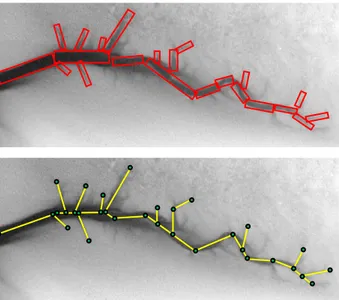
building footprints in Digital Surface Models (DSM) to our problem with the goal to find the configuration of rectangles which optimally fills the area of the fluvial network. The marked point process is realised by using a Reversible Jump Markov Chain Monte Carlo (RJMCMC) sampler coupled with a simulated annealing relaxation. As the extracted rectangles in our model usually do not overlap or touch each other, gaps typically occur in the result and the tidal network is not completely covered by rectangles. Furthermore, the network characteristic is not directly used in our approach yet. This is why we perform a second step and derive a final graph from the rectangles obtained in the first step (Fig. 1).
In the following, we first describe the mathematical foundation of the stochastic optimization using marked point processes (Section 2). We then present the proposed models for our data (Section 3.1) and the construction of a network graph (Section 3.2). In Section 4, we show some experiments and preliminary results on test data of the German Wadden Sea. Finally, conclusions and perspectives for future work are presented.
Figure 1. Outline of our proposed method: (1) the fitting of rectangles to the data by using a sampling process and (2) the construction of a network graph.
2. THEORETICAL BACKGROUND
2.1 Marked point process
In this section we give a brief introduction to marked point processes and their application for object detection tasks that is based on (Tournaire et al., 2010) and (Chai et al., 2013). For a formal definition of marked point processes the reader is referred to (Daley and Vere-Jones, 2003).
Informally speaking, a point process is a stochastic model describing a random configuration of points in a bounded region S (here: a digital image, thus the points xi exist in R2), where the number of points is also a random variable. In a Poisson point process, the number of points follows a discrete Poisson distribution with parameter (Chai et al., 2013). Given the number of objects, the locations are independent and identically distributed in S. In a marked point process, a mark mi is added to each point, typically a vector of parameters describing an object of a certain type that is also a multidimensional random variable. If we characterise an object ui = (xi, mi) by its location
and its parameters, a marked point process can be thought of as a stochastic model of configurations of an unknown number of such objects in S. In object detection, it is our goal to detect the most probable configuration of objects in a scene given the data. For that purpose, we need to define the probability density h of the marked point process. This can be achieved with respect to a reference point process, which is usually defined as a Poisson point process. The density function h is usually expressed using a Gibbs energy U(.) with . It can be modelled by the sum of a data energy Ud(.) and a prior energy Up(.) as used for instance by Mallet et al. (2009):
(1)
The relative influence of both energy terms is modelled by . The data energy Ud(.) measures the consistency of the object configuration with the input data. The energy Up(x) introduces prior knowledge about the object layout; our models for these two energy terms are described in Section 3. The optimal configuration of objects can be determined by minimizing the Gibbs energy U(.), i.e. . We estimate the global minimum by coupling a RJMCMC sampler and a simulated annealing relaxation.
2.2 Reversible Jump Markov Chain Monte Carlo
If the number of objects constituting the optimal configuration were known or constant, Markov Chain Monte Carlo (MCMC) sampling (Metropolis et al., 1953, Hastings, 1970) could be used for its determination. RJMCMC is an extension of MCMC that can deal with an unknown number of objects (Green, 1995). For that purpose, a Markov Chain (Xt), is simulated in the space of possible configurations. In each iteration t, the sampler proposes a change of the current configuration from a set of pre-defined types of changes accordingly to a density function, each of them associated with a density function Qi called kernel. Each kernel Qi is reversible, i.e. each change can be reversed applying another type of kernel. Following (Tournaire et al., 2010), we integrate three different types of change in our approach. First, an object can be added to or removed from the current configuration, which is accomplished by the birth and death kernels, Qb and Qd, respectively. Secondly, the parameters of an object of the current configuration can be modified (perturbation kernel Qp). A kernel Qi is chosen randomly according to a proposition probability which may depend on the kernel type. The configuration Xt is changed according to the kernel Qi, which results in a new configuration Xt+1. Subsequently, the Green ratio R (Green, 1995) is calculated:
In (2), Tt is the temperature of simulated annealing in iteration t
(cf. Section 2.3). The acceptance rate α of the new configuration
Xt+1 is computed from R using
Following Metropolis et al. (1953) and Hastings (1970) the new configuration Xt+1 is accepted with the probability α and rejected with the probability 1-α. The four steps of (1) choosing a proposition kernel Qi, (2) building the new configuration Xt+1, (3) computing the acceptance rate α, and (4) accepting or rejecting the new configuration are repeated until a convergence criterion is achieved.
2.3 Simulated Annealing
In order to find the optimum of the energy, the RJMCMC sampler is coupled with simulated annealing. For that reason, the parameter Tt referred to as temperature (Kirkpatrick et al., 1983) is introduced in equation 2. The sequence of temperatures Tt tends to zero as . Theoretically, convergence to the global optimum is guaranteed for all initial configurations X0 if
Tt is reduced (“cooled off”) using a logarithmic scheme. In
practice, a geometrical cooling scheme is generally introduced instead. It is faster and usually gives a good solution (Salamon et al., 2002; Tournaire et al., 2010).
3. METHODOLOGY
For the extraction of the tidal channel network we developed a two-step approach. In the first step, we optimally fit rectangles to the data using marked point processes (Section 3.1). Within the network each channel is represented by one or more rectangles with varying orientation, depending on the local direction of the channel. The optimization process minimizes a global energy function in the way described in Section 2.
If the model for the energy function describes the object configuration well, the tidal network will be almost completely covered by rectangles after step 1. However, the rectangles are not linked to each other, and there might be gaps between them. Thus, a result with a correct network structure is not guaranteed. That is why we apply a method for the derivation of a network representation in a second step (Section 3.2). For this purpose we consider the alignment of the rectangles and determine intersection points of the principal axes. The result is a graph where the nodes are points derived from the geometry of the rectangle configuration and the edges are straight line segments connecting these nodes.
3.1 Extraction of the network by sampling rectangles
We sample rectangles to the data using a RJMCMC sampler and simulated annealing as described in Section 2. Our model is based on (Tournaire et al., 2010), but it uses a different definition of the data energy, as will be pointed out in Section 3.1.1. In our method, a rectangular object ri is described by ri = (xi, mi), where the 2d vector xi describes the position of the centre of the rectangle in the image and the mark mi = (vxi, vyi, li) describes the shape and orientation of the rectangle by its semi-major axis (vxi, vyi) and its length ratio , li = l1i / l2i, where l1i and
l2i correspond to the short and long side length of the rectangle, respectively. In the sampling process rectangles are randomly added, removed or perturbed based on the criteria described in Section 2.2. Following Tournaire et al. (2010), there are only two possible types of perturbations: the first one carries out a shift and a change of the aspect ratio by a parallel shift of two corners connected by an edge, whereas the second one combines a rotation about one corner of the rectangle and a scaling. These moves are restricted by minimum and maximum values for the parameter of The birth kernel adds a new rectangle to the current configuration, whose parameters are sampled from prior distributions for the individual components of the mark. The parameter settings in our experiments are given in Section 4.3.
3.1.1 Data Energy: The data energy Ud(Xt) (equation 1) checks the consistency of the object configuration with the input data. Tidal channels are characterized by locally smaller heights and have high gradients on each bank and flat gradients between
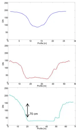
Figure 2. Typical profiles of tidal channels with different size in our test site. The digital numbers (DN) of the gray values of the DTM correspond to the heights z in the test site (here: DN = 0 and DN = 255 are equivalent to z =-0.02 m and z =1.72 m, so 1 DN corresponds to about 0.007 m).
these banks in the areas that may or may not be covered by water (depending on the tides). Typical profiles of tidal channels in our data are shown in Figure 2.
For the extraction of buildings, Tournaire et al. (2010) proposed a data term that enforced building outlines to correspond to large height gradients. A similar model can be applied here if the DTM (or the sign of the gradient) is inverted, with the difference that the absolute height differences are considerably lower in our case and that only the edges of the rectangles corresponding to the river banks will be determined by that model. Nevertheless, we model the data term for each edge of a rectangle in a similar way as Tournaire et al. (2010), just inverting the signs:
In (4), pi
m and pi
m+1
are two consecutive corners of the rectangle ri and is the component of the gradient of the DTM ( ) at pixel k in direction of the normal vector n of the edge . The normal vector is defined to point from the interior of the rectangle to the outside. The gradients are weighted by which corresponds to the rate of the edge length crossing the pixel k ( ) (Fig.3). The data term for one edge of the rectangle is the negative weighted sum of the gradient components for all pixels k along that edge. Our formulation differs from the
70 cm
one in (Tournaire et al., 2010) by the negative sign in (4). As stated above, this is necessary due to the fact that our objects, tidal channels, are deeper than the adjacent points in the DTM whereas buildings have a higher value in the DSM. The complete data energy for a rectangle is determined from
In equation 5 the constant weight ci is introduced. In (Tournaire et al., 2014), it corresponds to a minimum size of the overall façade surface for the buildings. In our application it is related to the minimum circumference of the rectangle multiplied by a small height change along the banks. In our experiments it was found out to be useful, though it has a different physical interpretation and, consequently, has to be set to a different value as in the original application.
Figure 3. The data term is calculated based on the gradient
of each pixel k and the normal vector of the rectangle
edge (the gray rectangle indicates a channel in the DTM).
3.1.2 Prior energy: Prior knowledge is integrated in the model by favouring an object configuration in which the objects do not overlap. For buildings this assumption is true because they can usually be represented by a single rectangle or can be made up of continuous or slightly overlapping objects. For the extraction of fluvial networks favouring non-overlapping objects makes sense, too, in order to avoid the accumulation of objects in regions with high data energy. Thus, as in (Tournaire et al., 2010), we model the prior energy of the configuration Xt by the sum of the overlap area a of neighbouring rectangles ri and rj
Here, the neighbourhood of a rectangle ri is defined by the set of rectangles intersecting ri.
3.2 Construction of a network graph
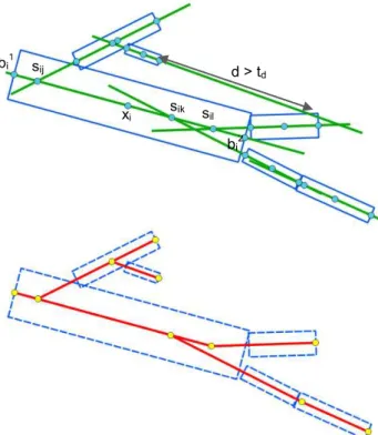
In a second step, we derive a network graph from the rectangles obtained in step 1. For this purpose we consider the alignment and the neighbourhood of each rectangle. The graph is constructed by introducing different criteria for the linking of points derived from the geometry of the rectangles. For each rectangle i we consider its centroid xi, its principal axis and the intersection points bi1 and bi2 of the principal axis with the border of the rectangle. Then, the principal axis is extended to the image boundaries. In each direction intersection points with other rectangles are calculated and the rectangle j with the closest intersection point is set as left or right neighbour of the current rectangle. In this way, each rectangle obtains one neighbour in each direction of the principal axis in case of an
existing rectangle in this direction. We represent the nodes of the final graph by three kinds of points: the intersection points si of principal axes of adjacent rectangles, the centroids xi and the intersection points of the principal axes with the rectangle border bi (Fig. 4). We do not consider all of these points for the graph construction, but rather choose points from each rectangle in the following way:
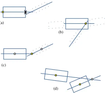
Choose the intersection point with the border bi only if there is no adjacent rectangle (Fig 5a).
If there are intersections points sij located inside the rectangle i and if these intersection points belong to a rectangle which is not the left or right neighbour of rectangle i,choose them (Fig 5b).
Choose all intersection points sij for which rectangle j is the right neighbour of rectangle i and i is the left neighbour of j. The only constraint is that sij has to be located between both rectangles' centroids (Fig. 5c).
Choose the centroids xi and xj in case of an existing adjacent rectangle and an intersection point sij which is not located between both centroids (Fig. 5d).
We also introduce a threshold td for the maximal distance d of two rectangles in case of an existing intersection point. If the distance between the closest points of the rectangle's border of two adjacent rectangles exceeds the threshold, the intersection point is not considered in the graph construction. In our experiments we set td = 50 m. In the next step the selected points are linked by edges based on different criteria:
Link all points within a rectangle.
Link the point which is furthest from the centroid with the closest point from the adjacent rectangle.
If the intersection point of two adjacent rectangles is outside one of the polygons, link the point which is furthest from the centroid with the closest point from the adjacent rectangle via the intersection point.
Figure 4. From the geometry of the rectangles different points are derived (top) and a final graph is constructed (bottom).
xi sij
bi1
bi2 sik sil
d > td pim
pim+1
n sk
.
(a)
(b)
(c)
(d)
Figure 5. Different criteria define the choice of the nodes for the network graph (points filled in yellow are chosen).
4. EXPERIMENTS
4.1 Test data
We evaluate our method on lidar data from the German Wadden Sea (Fig. 6). The test site is located in the south of the East Frisian island Norderney and covers an area of 1.0 km x 1.0 km. Many tidal channels of varying size are located in this area. Some of them extend over the entire test site with a width up to more than 100 m, whereas others exhibit a length of some tens of meters and a width in the range of only a few meters. The flight campaign took place in spring 2012 using a Riegl LMS-Q 560 sensor. The heights of the raw lidar point cloud (average point density 5.9 points / m²) are interpolated to generate a DTM of 1 m grid size. Within the DTM the height difference between the lowest and highest points is 1.74 m.
Figure 6: DTM of the test site in which the tidal channels have a low height. Some analyses are performed only for the outlined section area 1.
4.2 Evaluation
We analyse the applicability of the model of the sampling process for our test data and investigate different parameter settings. The result is evaluated based on the area of the tidal channel network which is covered by rectangles. For that purpose, we manually labelled the tidal channel network in the DTM in order to obtain reference data. The result of the sampling process is evaluated in a pixel-wise comparison with the ground truth data. All pixels inside the rectangles are considered as network pixels. For the determination of network pixels at the rectangle borders we use Bresenham's line algorithm (Bresenham, 1965). We calculate the number of correctly extracted network pixels (True Positive, TP) and non-network pixels (True Negative, TN) as well as the number of pixels incorrectly labelled as network pixels (False Positve, FP) and non-network pixels (False Negatives, FN). We also determine the correctness and completeness rate (Heipke et al., 1997) as well as the quality (Rutzinger et al., 2009) of the results. The generated network graph is not evaluated quantitatively, at this stage. In the future, it could be evaluated by constructing a buffer around the extracted edges and determining the length of all reference line segments inside the buffer (Grote et al., 2012).
4.3 Parameter settings
In our experiments, we set the parameter β in equation 1 to
β = 0.1 following Tournaire et al. (2010). The proposal probabilities of the kernels are set to = = 0.05 and = 0.9. Within the perturbation kernel all possible perturbations (cf. Section 3.1) are equally likely. The size of a rectangle is restricted by the maximum length of the short edge l1i. We set this value to 22 m which corresponds to the maximal channel width plus a puffer of 5 m in area 1. The initial weight ci in the data term (equation 5) and the maximal length ratio li max are varied in order to investigate their influence on the results.
4.4 Results
4.4.1 Extraction of the network by sampling rectangles
In the first investigation, we set the maximal length ratio li max =
1/5 andvary the initial weight ci in steps of 50 m. The results for area 1 after 3.5 million of iterations are shown in table 1. A low value of ci means that even structures with low height differences and, thus, a low façade surface can be extracted. That is why some rectangles are sampled in non-network areas and the correctness rate is low. This can be observed e.g. if the land surface is very rough and shows high height variations. With increasing correctness rate for higher values of ci, the completeness rate decreases. For high values of ci only the larger channels are extracted. The highest quality rate can be obtained for ci = 200 m², the result is shown in Figure 7. In the second investigation, we set ci = 200 m² and vary the maximal length ratio li max by increasing the denominator of the ratioin steps of 1 (Table 2). The completeness rate is increasing with increasing li max, too. The correctness rate decreases in general. The quality achieves is maximum for li max = 1/2. Here, the main tidal channel is approximate by short rectangles with are often too broad in the right part of the channel (Figure 7). Small, thin channels are not extracted with this value.
We also evaluate our method for the whole test site. Here, the parameter discussed above are set to li max = 5 and ci= 250 m², the number of iteration is set to 75 million. The computation area 1
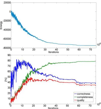
time was 190.1 seconds using the library LIBRJMCM (Brédif et al., 2012). Figure 8 (top) shows that the energy decreases and converges to a minimum after about 58 million iterations. Conversely, the completeness and quality rate increase (Figure 8, bottom). However, the correctness rate decreases after about 10 million iterations. We repeat the sampling process various times and obtain similar results. This indicates that the sampling process achieves the global minimum. However, the decreasing rate of correctness indicates that the energy model does not perfectly describe our problem and that an extension of the data and / or prior term is required. The best quality for the whole test site is achieved after 17.4 million iterations (Figure 9). Here, the quality is 49.7 % whereas the completeness and correctness rates are 60.6 % and 73.4 %, respectively. These relatively low accuracies can be mostly explained by the very broad channel at the top of the test site. Although we increased the parameter for the maximum length of the short edge l1i of a rectangle to 34 m, such a broad channel cannot be extracted. However, increasing this parameter too large would lead to a coarser result where predominantly large channels are detected. It can be seen that the strong hierarchy of our network is not described with our model yet. Moreover, our evaluation method should be refined, too. The tidal channels do not exhibit a completely rectangular footprint. Thus, the extracted rectangles give only an approximation of them and the evaluation of their areas results in False Positives at the rectangles borders inevitably. This limitation could be avoided by fitting other geometrical objects such as trapezoidal footprints to the data.
ci [m²] correctness
[%]
completeness [%]
quality [%]
0 18.7 94.5 18.5
50 34.6 85.3 32.6
100 54.7 80.5 48.3
150 69.1 79.2 58.5
200 78.2 77.9 64.0
250 81.4 69.9 60.2
300 82.5 65.4 57.4
350 81.3 66.2 57.5
400 82.2 63.3 55.7
450 81.2 63.9 55.7
500 80.4 58.8 51.5
Table 1. Results for area 1 varying the weight ci in the data term.
Figure 7. Results for area 1 with the parameter ci = 200 m² and
li max = 1/5 (top) and for ci = 200 m² and li max = 1/2 (bottom) (black = TP, yellow = FP, red = FN, gray = TN).
li max correctness [%]
completeness [%]
quality [%]
1/2 70.1 62.6 49.4
1/3 69.8 71.8 54.8
1/4 77.6 73.0 60.3
1/5 78.2 77.9 64.0
1/6 59.7 76.4 50.4
1/7 82.7 75.8 65.5
1/8 67.9 76.9 56.5
1/9 49.5 82.4 44.8
1/10 50.2 83.4 45.7
Table 2. Results for area 1 varying the maximal length ratio li maxof the rectangle's edges in the sampling process.
Figure 8. The modelled energy converges for increasing iterations (top). The completeness and quality rate increase while the correctness rate is decreasing (bottom).
Figure 9. Result for the whole test site (black = TP, yellow = FP, red = FN, gray = TN).
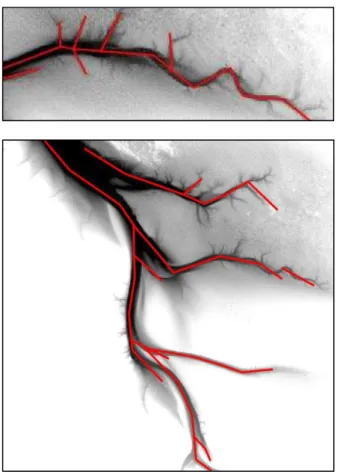
4.4.2 Construction of a network graph
From the extracted rectangles a network graph is constructed based on criteria offered in Section 3.2. The results are shown in Figure 10. For area 1 and the whole test site the edges mostly correspond to the skeleton of the tidal channels. All line segments are connected or can be connected outside the DTM. In the whole test site, an isolated line segments occur on the right site due to the parallel major axes to the adjacent rectangles and, thus, no intersection point.
Figure 10. Constructed network graph for area 1 (ci = 200,
li max = 7, iterations = 35 million) and the whole test site (ci = 250, li max= 5, iterations = 17.4 million)
5. CONCLUSION AND OUTLOOK
In this paper, we presented a method for the automatic extraction of tidal channels in a DTM. In a first step, we fit rectangles to the data using a sampling method based on marked point processes. A network graph is derived afterwards. Our results show a proof of concept of our stochastic approach. We intend to improve our model in a number of ways. The data term has to be extended by a homogeneity criterion of the pixels inside the rectangles. In addition, we plan to take into account the hierarchical structure of the network, as channels with strongly varying width cannot be extracted with the same parameter settings yet. The results of the derived network graph have shown that the topology of the tidal channel network is not always correctly described by our defined criteria. Furthermore, the connectivity of all channels is not guaranteed. That is why we intend to integrate this characteristic directly in the sampling process. In this context, graph based approaches which model the network structure in the prior term look promising (e.g. Chai et al., 2013). Our data offers additional constraints like a tree
structure of the network which we want to integrate in our model. We also plan to consider the flow direction of the water between adjacent objects.
ACKNOWLEDGEMENTS
We would like to thank the Lower Saxon State Department for Waterway, Coastal and Nature Conservation (NLWKN) for providing the lidar data.
We used the "LIBRJMCM: An Open-source Generic C++ Library for Stochastic Optimization ", developed by Mathieu Brédif and Olivier Tournaire (Brédif and Tournaire, 2012).
REFERENCES
Ashley, G. M., Zeff, M. L., 1988. Tidal channel classification for a low-mesotidal salt marsh. Marine Geology, 82, pp. 17–32.
Brédif, M., Tournaire, O., 2012. Librjmcmc: An Open-source Generic C++ Library for Stochastic Optimization. International Archives of the Photogrammetry, Remote Sensing and Spatial
Information Sciences, Vol. XXXIX-B3, pp. 259–264.
Bresenham, J. E., 1965. Algorithm for computer control of a digital plotter. IBM Systems Journal 4 (1), pp. 25–30.
Chai, D., Foerstner, W., and Lafarge, F., 2013. Recovering line-networks in images by junction-point processes. IEEE Conference on Computer Vision and Pattern Recognition (CVPR), Portland.
Daley, D. J., Vere-Jones, D., 2003. An Introduction to the Theory of Point Processes: Elementary Theory and Methods, Springer.
Fagherazzi, S., Bortoluzzi, A., Dietrich, W. E., Adami, A., Lanzoni, S., Marani, M., Rinaldo, A., 1999. Tidal Networks 1. Automatic network extraction and preliminary scaling features from digital terrain maps. Water Resources Research. 35, pp. 3891–3904.
Green, P., 1995. Reversible Jump Markov Chains Monte Carlo computation and Bayesian model determination. Biometrika, Vol. 82(4), pp. 711–732.
Grote, A., Heipke, C., Rottensteiner, F., 2012. Road Network extraction in suburban areas, Photogrammetric Record. The
Photogrammetric Record 27(137), pp. 8-28.
Hastings, W., 1970. Monte Carlo sampling using Markov chains and their applications. Biometrika, Vol. 57(1), pp. 97– 109.
Heipke, C., Mayer, H., Wiedemann, C. and Jamet, O., 1997. Evaluation of automatic road extraction. In: Proc. ISPRS Workshop 3D Reconstruction and Modeling of Topographic Objects, Stuttgart, Germany, Sep. 17–19, Vol. XXXII/3–4W2,
Int. Archives Photogrammetry Remote Sens., pp. 151–160.
Kirkpatrick, S., Gelatt, C. D., Vecchi, M. P., 1983. Optimization by Simulated Annealing. Science 220, pp. 671-680.
Lacoste, C., Descombes, X., Zerubia, J., 2005. Point processes for unsupervised line network extraction in remote sensing. The International Archives of the Photogrammetry, Remote Sensing and Spatial Information Sciences, Volume XL-3, 2014
IEEE Trans. on Pattern Analysis and Machine Intelligence, Vol. 27, No. 2, pp. 1568–1579.
Lafarge, F., Descombes, X., Zerubia, J., Pierrot-Deseilligny, M., 2008. Building reconstruction from a single DEM. IEEE CVPR.
Lohani, B., Mason, D. C., Scott, T. R., Sreenivas, B., 2006. Identification of tidal channel networks from aerial photographs alone and fused with airborne laser altimetry. International Journal of Remote Sensing 27 (1), pp. 5–25.
Mallet, C., Lafarge, F., Roux, M., Soergel, U., Bretar, F. Heipke, C., 2010. A marked point process for modeling lidar waveforms, IEEE Transactions on Image Processing, 19 (12), pp. 3204–3221.
Mason, D. C., Scott, T. R. and Wang, H.-J., 2006. Extraction of tidal channel networks from airborne lidar data. ISPRS Journal
of Photogrammy and Remote Sensing, Vol. 61, 2, pp. 67–83.
Metropolis, M., Rosenbluth, A., Teller, A., and Teller, E., 1953. Equation of state calculations by fast computing machines, Journal of Chemical Physics, Vol. 21, pp. 1087–1092.
Perrin, G., Descombes, X., Zerubia, J., 2005. Adaptive simulated annealing for energy minimization problem in a marked point process application. Proc. Energy Minimization
Methods in Computer Vision and Pattern Recognition, St
Augustine, United States.
Rutzinger, M., Rottensteiner, F., Pfeifer, N., 2009. A comparison of evaluation techniques for building extraction from airborne laser scanning. IEEE Journal of Selected Topics in Applied Earth Observations and Remote Sensing, 2, pp. 11-20.
Salamon, P., Sibani, P., Frost, R., 2002. Facts, Conjectures and Improvements for Simulated Annealing. Society for Industrial
and Applied Mathematics, Philadelphia, USA.
Sun, K., Sang, N., Zhang, T. (2007). Marked point process for vascular tree extraction on angiogram. Conference on computer vision and pattern recognition, pp. 467–478.
Tournaire, O., Paparoditis, N., Lafarge, F., 2007. Rectangular road marking detection with marked point processes. International Archives of Photogrammetry, Remote Sensing and Spatial Information Sciences, 36 (Part 3/W49A), pp. 73–78
Tournaire O., Bredif, M., Boldo D., Durupt, M., 2010. An efficient stochastic approach for building footprint extraction from digital elevation models. ISPRS Journal of
Photogrammetry and Remote Sensing, Vol. 65, 4, pp.317 -327.