International Journal for Quality research UDK- 921.9.02 005.6
Short Scientific Paper (1.03)
Ľ
ubomír Šooš
Iveta Onderova
Slovak university of technology, Slovac Republic
Parameters Influencing the Components of Quality
Abstract:
At present there is a permanently increasing
demand from machine-tool users for metalworking and
fabrication machines for high speed cutting (HSC), which
are the basic trend of the intensification of processes that
means shortening of cycle times. The progress in building
and applications of a new generation of machines was
enabled by new cutting materials and tools, high revolution
spindles, sophisticated types of leading, linear drives, etc.
Actually, this progress is remarkable when it comes to the
increase of the output of energy beam sources (laser,
plasma, water beam) in the machines for cutting of
material. That also increases demands for highly effective,
high dynamic technological tables that create the support
for cutting heads, while the demands for the quickness of
these tables are extremely high with speeds up to 300
m/min.
Keywords:
Quality System, quality of the product surface
1. INTRODUCTION
Numerically controlled linear axes are becoming an inseparable part of the present production machines. The quality of the final products depends also on the quality of manufacturing of these axes. Qualitative parameters of the product, influenced by numerically controlled machine parts, may be subdivided into the quality of the product surface and into the quality of the spatial precision of the manufacturing. The spatial precision of the product depends to a large extent on the precision of the positioning of the linear axes of the machine. Herewith the precision of the linear axes positioning is one of the most important parameters of the numerically controlled axes and thus one of the most important parameters influencing the quality of the products.
2. EXPERIMENT
On the Microstep s.r.o. company equipment, measurements of two linear axes
have been performed. It is a laser cutting machine in a three-axe version. It is a development equipment, on which the company tests using of linear axes with linear motors.
Total range of axis y 1500 mm Total range of axis x 3000 mm Rate of working do 260m/min
Acceleration 25 m/s2
Resolution of position sensor 0,000488 mm Max. tolerance mistake It tests.
Table 1 – Basic data about the machine.
3.1 Standards and accuracy of positioning
The International Standard ISO 230 Test code for machine tools specifies methods of testing parameters of machine tools. [2]. The Standard consists of the fifth parts, which deal with evaluation different parameters of machine tools:
geometric accuracy of machines operating under no-load or finishing conditions,
determination of accuracy and repeatability of positioning of numerically controlled axes,
evaluation of thermal effects,
circular tests for numerically controlled machine tools,
noise emissions.
In term of accuracy of measurement is the most interesting the second part of this standard, and it is ISO 230-2:2006 Determination of accuracy and repeatability of positioning numerically controlled axes.
This part of standard specifies methods of testing, evaluating the accuracy and repeatability of positioning of numerically controlled machine tool axes by direct measurement of individual axes on the machine. The methods described apply equally to linear and rotary axes.
3.2. Test conditions
Standards (ISO 230-2:2006, STN 20 0300-31) introduce mainly specifications of measurement, for example the room temperature and trim of machine etc.[2],[3].
It is recommended that the supplier/manufacturer offer guidelines regarding what kind of thermal environment should be acceptable for the machine to perform with the specified accuracy.
Ideally, all dimensional measurements are made when both the measuring instrument and the measured object are soaked in an environment at a temperature of 20 °C. If the measurements are taken at temperatures other than 20 °C, then correction for nominal differential expansion (NDE) between the axis positioning system and the test equipment must be applied to yield results corrected to 20 °C. This condition requires temperature measurement of the representative part of the machine positioning system as well as the test equipment.
It should be noted, however, that any temperature departure from 20 °C can cause an
additional uncertainty related to the uncertainty related to the uncertainty in the effective expansion coefficient used for compensation. A typical value for the resulting uncertainty is ± 2 µm. Therefore the actual temperatures shall be recorded in the test report. The machine tool supplier/manufacturer should supply the effective expansion coefficient of the axis positioning systems.
The machine and, if relevant, the measuring instruments shall have been in the test environment long enough to have reached a thermally stable condition before testing. They shall be protected from draughts and external radiation such as sunlight, overhead heaters, etc.
Standard ISO 230-2:2006 defines two practices of measurement in dependence on range of linear axes, and it:
range up to 2000 mm,
rozsah exceeding 2000 mm.
3.3. Tests for linear axes up to 2 000 mm
On controlled axes of travel up to 2 000 mm standard ISO 230-2:2006 dictates measurement a minimum of tive target positions per meter. For the target position Pi it is necessary to make minimum five measurements. Where the value of each target position can be freely chosen, it shall take the general form:
Pi = ( i - 1 ) p + r where:
Pi - target position,
i - the number of the current target position,
p - an interval based on a uniform spacing of target points over the measurement travel,
r - takes a different value at each target position, yielding a non uniform spacing of the target positions over the measurement travel to ensure that periodic errors are adequately sampled.
Figure 2 - Standard test cycle
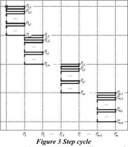
3.4. Step cycle
The results from tests made using this method may be different those obtained from the standard test cycle shown in figure 2.
With the standard test cycle, the approach to the extreme target positions from opposing directions takes place with a large difference in time intervals. However, with the step cycle the approach to the target positions from either direction takes place wihin shorter time intervals and a longer time is taken between the measurements of the first and the last target positions.
Figure 3 Step cycle
Measurements according to the standard test cycle may reflect thermal influences which affect differently the various target positions along the axis under test. Here thermal influences during the measurements
may be evident in both the reversal values B and the repeatability R.
In the case of the step cycle, thermal influences may be evident in the range of the mean bidirectional positional deviation, M, whereas the reversal values and repeatability will be only slightly affected by the thermal behaviour of the machine.
3.5. Tests for linear axes exceeding 2 000 mm
For controlled axes longer than 2 000 mm, the whole measurement travel of the axis shall be tested by making one unidirectional approach in each direction to target positions selected according to (1), with an average interval length p =250 mm. Approach tu target position is realizes in both of them direction. The measurement performs at least five times every way.
3.6. Measuring data evaluation For every target position is evaluating measuring date particularly for every directions. As a result of evaluation is measuring data and limitation of deviation.
↑
+
↑
ii
s
x
2
and
x
i↑
−
2
s
i↑
and↓
+
↓
ii
s
x
2
and
x
i↓
−
2
s
i↓
where:
x
i- deviation in a point i, si – standard deviation in a point i.
For axis up to 2 000 mm they are not forecast standard indeterminateness, repeatability and accuracy applied.
Figure 4 – Bidirectional accuracy and repeatability of positioning, normative ISO
230-2:2006
3.7. Regression analysis
positioning deviation in the whole extent of the measured axis, but only in the measured points. The positioning deviation between these points is not known, the standard however assumes a linear course of the positioning deviation value between the measured data. This is not correct from the point of view of the evaluation of the measured data. It is therefore appropriate to use regress analysis for an estimation of the positioning precision also outside of measured points.
3.8. Estimation of regression curve parameters
A possible solution how to find out the state of the positioning precision also between measured points is a linkage of the regress curve through measured deviations.
The regression curve Δ(P) is a positioning deviation in an arbitrary point and may be proposed in the following form:
n n
P
b
P
b
P
b
b
Δ
=
+
⋅
+
⋅
2+
K
+
⋅
2 1
0 where:
bi, i = 1,...n – are unknown multi-nominal parameters,
P – is a point in which the deviation is calculated.
The measured deviations in the points are plugged in the equation and thereby the equation transfers to a system of equations.
n n
P
b
P
b
P
b
b
Δ
1 2 1 2 1 1 01
=
+
⋅
+
⋅
+
K
+
⋅
n n
P
b
P
b
P
b
b
Δ
2 2 2 2 2 1 02
=
+
⋅
+
⋅
+
K
+
⋅
.... n m n m m
m
b
b
P
b
P
b
P
Δ
=
+
⋅
+
⋅
2+
K
+
⋅
2 1
0 where:
Δ
i, i = 1,...m - the deviation value is determined as an arithmetic average of the measured data in the point Pi.Then for the regress curve parameters equation estimation by means of a smallest squares method the following relation is valid:
Δ
x
x
x
b
ˆ
=
(
T)
−1 T where:
b
ˆ
- is a vector of an estimation of the unknown multi-nominal parameters, x – is a matrix containing the measurement points in a multi-nominal form.
In this case the weight of the individual
measurements is however not considered and therefore it is appropriate to extend the relation by a covariance matrix U(Δ). Then this relation transfers to the following form.
Δ
U
x
x
U
x
b
ˆ
=
(
T −1(
Δ
)
)
−1 T −1(
Δ
)
where matrix has form:⎟⎟
⎟
⎟
⎟
⎠
⎞
⎜⎜
⎜
⎜
⎜
⎝
⎛
=
nb
b
b
M
1 0ˆ
b
Multi-nominal x proposal matrix has the following form:
⎟
⎟
⎟
⎟
⎟
⎠
⎞
⎜
⎜
⎜
⎜
⎜
⎝
⎛
=
n m m n nP
P
P
P
P
P
K
M
M
M
M
K
K
1
1
1
2 2 1 1x
Matrix of the measured values Δ has the following form:
⎟⎟
⎟
⎟
⎟
⎠
⎞
⎜⎜
⎜
⎜
⎜
⎝
⎛
=
mΔ
Δ
Δ
M
2 1Δ
Covariance matrix U(Δ) has the following form: ⎟ ⎟ ⎟ ⎟ ⎟ ⎟ ⎠ ⎞ ⎜ ⎜ ⎜ ⎜ ⎜ ⎜ ⎝ ⎛ = − − ) ( ) , ( . . ) , ( ) , ( . . . . ) , ( ) , ( ) ( ) , ( ) , ( ) , ( ) , ( ) ( ) ( 2 1 1 1 2 3 2 2 2 1 2 1 3 1 2 1 1 2 m m m m m m m m Δ u Δ Δ u Δ Δ u Δ Δ u Δ Δ u Δ Δ u Δ u Δ Δ u Δ Δ u Δ Δ u Δ Δ u Δ u M M M M M L L Δ U
The covariance matrix contains uncertainties which are on the diagonal and in the remaining part there are covariances between the individual measurements. The measurements are often not correlated, then
Covariance matrix U(bˆ) unknown multi-nominal parameters, b0... bn calculated as:
1 1 T
)
)
(
(
)
ˆ
(
b
=
x
U
−x
−U
Δ
Where covariance U(Δˆ) matrix has the following form: ⎟⎟ ⎟ ⎟ ⎟ ⎟ ⎟ ⎠ ⎞ ⎜⎜ ⎜ ⎜ ⎜ ⎜ ⎜ ⎝ ⎛ = − − ) ˆ ( ) ˆ , ˆ ( . . ) ˆ , ˆ ( ) ˆ , ˆ ( . . . . ) ˆ , ˆ ( ) ˆ , ˆ ( ) ˆ ( ) ˆ , ˆ ( ) ˆ , ˆ ( ) ˆ , ˆ ( ) ˆ , ˆ ( ) ˆ ( ) ˆ ( 2 1 1 1 2 3 2 2 2 1 2 1 3 1 2 1 1 2 m m m m m m m m b u b b u b b u b b u b b u b b u b u b b u b b u b b u b b u b u M M M M M L L b U
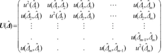
Covariance matrix U(Δˆ)estimate deviation of positioning calculated as:
T x ) bˆ ( xU = ) Δˆ ( U
Where covariance matrix U(Δˆ) has the following form:
⎟⎟ ⎟ ⎟ ⎟ ⎟ ⎟ ⎠ ⎞ ⎜⎜ ⎜ ⎜ ⎜ ⎜ ⎜ ⎝ ⎛ = − − ) ˆ ( ) ˆ , ˆ ( . . ) ˆ , ˆ ( ) ˆ , ˆ ( . . . . ) ˆ , ˆ ( ) ˆ , ˆ ( ) ˆ ( ) ˆ , ˆ ( ) ˆ , ˆ ( ) ˆ , ˆ ( ) ˆ , ˆ ( ) ˆ ( ) ˆ ( 2 1 1 1 2 3 2 2 2 1 2 1 3 1 2 1 1 2 m m m m m m m m Δ u Δ Δ u Δ Δ u Δ Δ u Δ Δ u Δ Δ u Δ u Δ Δ u Δ Δ u Δ Δ u Δ Δ u Δ u M M M M M L L Δ U
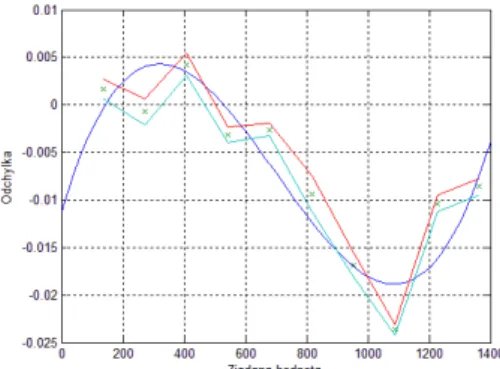
The result of this analysis is a regression curve which considers the weight of the individual points and also the trend of their direction and therefore it may be stated that it describes also the measured parameter behaviour – linear axis positioning precision also between measured points.
Figure 5 - Evaluation of the measured after applied regres analysis 3rd degree one
3.9. Evaluation of the measured data
3.10 Evaluation of the measured data with use of regression analysis A solution how to get a description of
the deviation also between measured points is a linkage of the regress curve through measured deviations. This is possible by using the smallest squares method. In order to be able to use this method, there has to be a regress multi-nominal degree determined.
3.11. Regression for multi - nominal degree determination By the regression for multi-nominal degree determination it is started from a regress multi-nominal maximum degree limitation. In our case on the x axis there are 10 points measured. It means that there cannot be a curve with a higher degree than 10 linked through them, because there would not be a sufficient number of independent equations for the multi-nominal coefficient determination. Equally for the y axis which has 11 measured points, the maximum multi-nominal degree is equal to 11. By these degrees by it would not be a regression but a linkage of a curve by points because the system would not be over-determined but over-determined. Therefore there were maximum multi-nominal degrees at the level of 8th of 9th degrees selected.
The residual dispersion and individual criteria values for the individual axes and multi-nominal degrees for the axis x are stated in the table 3 and in the table 4.
According to the calculated values by approximation from the right a 7th degree multi-nominal results, because the criteria by this degree gained the minimum value. Also for approximation from the left all three criteria indicate a 7th degree multi-nominal.
Figure 6 - Displacement curve 2 a 7 degree. Values are in mm.
For the y axis a zero degree multi-nominal resulted for approximation from the right as well as from the left. This cannot however capture the curve trend, and therefore it is more appropriate to use a higher degree multi-nominal, e.g. a 3rd degree one.
3.12. Regress multi-nominal linkage
On a basis of the criteria there was a 2nd degree multi-nominal used for the regress analysis. On the following graphs, there are measured and calculated values depicted.
Figure 7 - Regress multi-nominal linkage
Figure 8 - - Comparison of multi-nominal 3 a 4 degree, value are in mm
Figure 9 - Comparison of multi-nominal 3 a 4 degree, value are in mm
CONCLUSION
Nowadays we are preparing one experiment for the verification of the calculated data will be executed in the next phase of solving of the project that consists of experimental measuring of real movements and strains of the portal along the y axis using strain-gauge sensors.
Acknowledgement
The research work described in the paper was performed by a financial support of the grant VEGA 1/0265/08