www.nonlin-processes-geophys.net/18/911/2011/ doi:10.5194/npg-18-911-2011
© Author(s) 2011. CC Attribution 3.0 License.
in Geophysics
Bias correction and post-processing under climate change
S. Vannitsem
Institut Royal M´et´eorologique de Belgique, Avenue Circulaire, 3, 1180 Brussels, Belgium Received: 5 August 2011 – Accepted: 25 November 2011 – Published: 2 December 2011
Abstract. The statistical and dynamical properties of bias correction and linear post-processing are investigated when the system under interest is affected by model errors and is experiencing parameter modifications, mimicking the poten-tial impact of climate change. The analysis is first performed for simple typical scalar systems, an Ornstein-Uhlenbeck process (O-U) and a limit point bifurcation. It reveals sys-tem’s specific (linear or non-linear) dependences of biases and post-processing corrections as a function of parameter modifications. A more realistic system is then investigated, a low-order model of moist general circulation, incorporating several processes of high relevance in the climate dynam-ics (radiative effects, cloud feedbacks...), but still sufficiently simple to allow for an extensive exploration of its dynamics. In this context, bias or post-processing corrections also dis-play complicate variations when the system experiences tem-perature climate changes up to a few degrees. This precludes a straightforward application of these corrections from one system’s state to another (as usually adopted for climate pro-jections), and increases further the uncertainty in evaluating the amplitudes of climate changes.
1 Introduction
Long term measurement environmental records indicate that climate is experiencing modifications on a wide variety of time and space scales. Under this changing environment, one can wonder whether how predictable is the system. In this context, two types of questions arise: (i) what are the mod-ifications of the statistical and dynamical properties of the system under slow variations of its forcings, usually referred
Correspondence to:S. Vannitsem ([email protected])
as system’s sensitivity, and (ii) can we predict the slow mod-ifications of the system.
If the model at hand representing the dynamics of real-ity is good enough and if we have a good knowledge about the uncertainty in the forcings and in the initial conditions, one could imagine to perform projections to get a reliable estimate of the possible outcomes. However models are al-ways affected by model errors, increasing the uncertainty on the possible outcome (see e.g. Stainforth et al., 2007; Knutti et al., 2008), in particular in case of (non-linear) sys-tems that could experience catastrophic changes (i.e. bifur-cations). These errors may indeed considerably affect the specific structure of the system’s attractor and of its bifur-cation diagram. Their presence is amply demonstrated by the difficulty of atmospheric models in reproducing correctly the climate, as illustrated by the robust systematic errors that are still present in the climate of state-of-the-art models (e.g. Berner et al., 2008).
One can therefore wonder whether this type of post-processing can still be used in the context of a transient cli-mate, in particular in the context of decadal forecasts. The obvious answer would be no in a strict sense since modifica-tions of external parameters generically imply modificamodifica-tions of the variability of the system. But in view of the strong ne-cessity and pressure in getting answers on the potential im-pact of climate changes on our society, these post-processing are used assuming that the impact of model errors is the same before and after the climate change, or is varying linearly in time (Buser et al., 2009). An interesting attempt in un-derstanding the dependence of the bias on the temperature and precipitation amplitudes has been performed by Chris-tensen et al. (2008) in the context of current climate simu-lations. This experiment, although not realistic since it does not compare biases before and after climate change, has en-lightened the possible nonlinear character of the model bi-ases as a function of increasing temperatures or precipitation amounts.
In the present work, the statistical and dynamical proper-ties of bias correction and linear post-processing, in the pres-ence of model errors, are investigated when the system under interest is experiencing parameter modifications, mimicking the potential impact of climate change. The sources of model errors are restricted here to parametric errors. Section 2 is devoted to the analysis of simple typical scalar systems, an Ornstein-Uhlenbeck process (O-U) and a limit point bifur-cation (both paradigms of important processes acting in the atmosphere and climate). The analysis reveals (potentially) complicate dependences of biases and post-processing cor-rections under parameter evolution. The investigation of a more realistic system, the low-order model of moist general circulation developed by Lorenz (1984) briefly described in the Appendix, also supports this statement (Sect. 3). This system is incorporating several processes of high relevance in the climate dynamics (radiative effects, cloud feedbacks...), but is still sufficiently simple to allow for an extensive ex-ploration of its dynamics. The conclusions are then drawn in Sect. 4.
2 Post-processing in scalar systems 2.1 Bias correction
Bias correction is certainly the simplest approach to post-process weather forecasts or climate runs. It simply consists in removing the mean of an ensemble of previous forecasts from current forecasts or of long climate runs. How this bias is affected by climate modifications is the central question of this section in the context of scalar systems.
2.1.1 Ornstein-Uhlenbeck process
Let us consider first the case where the real dynamics and its model are described by Ornstein-Uhlenbeck processes,
dx
dt = −λx+K+ξ (1)
dy
dt = −λ
′y+K′+ξ′ (2) whereξ andξ′are white noise processes such that
< ξ(t ) >=< ξ′(t ) >=0
< ξ(t )ξ(t′) >=Q2δ(t−t′)
< ξ′(t )ξ′(t′) >=Q′2δ(t−t′)
where< . >refers to an ensemble average. The evolution of the probability densities of the solutions of these equations is described by a Fokker-Planck equation and the moments of the distribution can then be evaluated (e.g. Gardiner, 1985). Let us focus first on the properties of the first moments,
d < x >
dt = −λ < x >+K (3)
d < y >
dt = −λ
′< y >+K′ (4)
Assume furthermore that the parameterK is constant and identical toK′. The asymptotic stationary solutions are then staigthforwardly obtained,xs=K/λandys=K/λ′, which
gives aclimate biasof
(xs−ys)K=K
λ−λ′
λλ′ (5)
Let us now assume that the dynamical change is expressed as a jump in the value of K,K′′=K+δK. Under these circumstances, the bias is given by
xs′−ys′=(K+δK)λ−λ
′
λλ′
=(xs−ys)K+δK
λ−λ′
λλ′ (6)
indicating that the bias depends linearly on the “climate” per-turbationδK. This straightforward analysis already suggests that the bias is not a stationary quantity, as often assumed in the climate community when working with anomalies. Let us now consider that the model error is present in the parameter
K,δK=K′−Kand the climate perturbation will affect the parameterλ. Assuming for simplicity thatλ=λ′and that the new parameter value after the change is given byλ′′=λ+δλ, one gets
(xs−ys)λ =
δK
λ (7)
(xs′−y′s)λ =
δK
(λ+δλ)
=(xs−ys)λ−
δKδλ
λ +
δKδλ2
λ +O(δλ
3)
indicating a nonlinear dependence of the bias on the climate perturbation, imposed throughδλ.
Up to now, climate change was expressed in the form of an abrupt change of a parameter, but usually parameter changes are time dependent, such as the CO2 increase supposed to
affect the global temperature as a linear time dependent forc-ing (see Nicolis, 1988, for a discussion on this point). There-fore let us now consider that one has a climate change ex-pressed through a progressive increase of the additive pa-rameter in the form ofa ramp, namely thatK=γ+ǫt and
K′=γ+ǫ′t and the model error is incorporated in the pa-rameter valueλ,λ′=λ+δλ. Note that for completeness the climate change scenario is also affected by an uncertainty in-corporated through a modification of the parameterǫ. In this case, the solutions of Eqs. (3)–(4) are given by
< x(t ) >=< x(0) > e−λt+γ
λ(1−e
−λt)
+λǫ[e
−λt
λ +(t−
1
λ)]
< y(t ) >=< y(0) > e−λ′t+γ
λ′(1−e−
λ′t)
+ ǫ
′
λ′[
e−λ′t
λ′ +(t−
1
λ′)]
(9) and the time dependent bias is the difference between the two equations. For times larger than 1/λand 1/λ′, one gets
< y(t ) >−< x(t ) >≈γλ−λ
′
λλ′ +(
ǫ′
λ′−
ǫ
λ)t
−(ǫ
′
λ′2−
ǫ
λ2) (10)
Clearly a (linear) time dependence of the bias is present that will depend on the amplitude of the model errorδλ, the ramp velocityǫand the uncertainty of the ramp velocityδǫ=ǫ′−
ǫ.
These results indicate that even in a linear system, a non trivial dynamics of the bias associated with the modelling error is present under climate change. This feature contrasts with the classical view that the bias associated with model deficiencies are similar under climate change.
For comparison let us also consider the case of a multi-plicative ramp. The evolution equation for the first moment of the O-U process is
d < x >
dt = −(λ+ǫt ) < x >+K (11)
The formal solution involves error functions that are not very transparent. One therefore resorts to an adiabatic for-mulation – considering that the parameterǫis small – in or-der to get the solution for long times (Nicolis and Nicolis, 2000). It consists in transforming the time asτ=λ+ǫtand seeking for a solution of the form
< x >=< x >0+ǫ < x >1+... (12)
Equating the terms corresponding to the same order inǫ, one gets for the two first orders,
< x >0=
K
τ (13)
< x >1=
K
τ3 (14)
Note that< x >0is simply the stationary solution of Eq. (11),
and is referred as theadiabatic approximation. Similar ex-pansion can be performed for the model version of Eq. (11) in which the parameters are modified (becomingK′andǫ′). The modification of the bias in time up to the first order inǫ
andǫ′is now given by
< y > (t )−< x > (t )≈ K
′
λ+ǫ′t−
K
λ+ǫt
+( ǫ
′K′
(λ+ǫ′t )3−
ǫK
(λ+ǫt )3) (15)
revealing a complicate non-linear variation in time, even in the case of this simple linear system.
2.1.2 A prototypical non-linear system
Assume now that the system under consideration displays a limit point bifurcation. This is one typical bifurcation, known to play an important role in many components of the climate systems and in particular in the Ocean dynamics (e.g. Dijk-stra, 2005; Dijkstra and Ghil, 2005). In the absence of fluc-tuations, it obeys a normal form (see Nicolis, 1988),
dx
dt =x(x−m)+K (16)
whose steady state solutions are given by
x±=1
2[m± p
m2−4K] (17)
Let us now assume that a model error is present in m, the model steady states are then given by
y±=1
2[m ′±p
m′2−4K′] (18)
Let us focus on the stable branch of solution and one as-sumes that parametersK andK′ are progressively increas-ing in time,K=γ+ǫtandK′=γ+ǫ′t. In order to clarify analytically the properties of the bias, one resorts to the adia-batic approximation – considering that the parametersǫand
ǫ′are small – in order to get the solution for long times. Up to the first order inǫ, one gets
x0=
1 2[m−
p
m2−4τ] (19)
x1= −
1
m2−4τ (20)
y0=
1 2[m
′−p
m′2−4τ′] (21)
y1= −
1
whereτ=γ+ǫtandτ′=γ+ǫ′tare the rescaled times. The bias is therefore approximately equal to
y−x ≈(1
2[m ′−p
m′2−4τ′] −1
2[m− p
m2−4τ])
+( −ǫ
′
m′2−4τ′−
−ǫ
m2−4τ) (23)
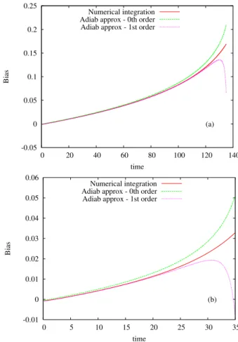
This relation is represented in Fig. 1 as a function of time, together with the direct numerical integration of the system defined by Eq. (16) and its model version for different values ofǫ andǫ′. First it clearly indicates the nonlinear charac-ter of the bias under climate change expressed in the form of a ramp. Second, relation (23) is a good approximation of the variation of this bias. This relation displays a com-plicate structure far from the simple approximation made in the literature, namely constant bias or linear variation of the bias (Buser et al., 2009). Note that a similar analysis can be performed when parametermis affected by the climate modification with similar conclusions. It also clearly sug-gests that the temporal variation of the bias highly depends on the velocity increase of the parameter affected by the cli-mate change (as for the O-U process with multiplicative ramp presented in the previous section). This further complicates the evaluation of the bias and of the future climate trends. 2.2 Linear post-processing
Usually the mean of the process is not the only moment af-fected by the presence of model errors. One could therefore have a need to correct higher order moments too, and in par-ticular the variance of the field of interest.Under stationary conditions, linear post-processing can allow for providing the correction of both the mean and the variance as discussed in Vannitsem (2009) for weather forecasts. These approaches can be extended to seasonal or decadal forecasts, but in the later case changes in system forcings (i.e. increase of anthro-pogenic gases) could affect the potential of correction.
Let us assume that before any climate change, one can de-velop a linear post-processing algorithm for a forecast, al-lowing for the correction of both the mean and the variance of the field of interest,
XC′(t )=α′(t )+β′(t )XM(t ) (24)
wheretrefers to the lead time of the forecast,XMthe model
predictor, and the parameters α′(t ) and β′(t )are obtained by minimizing a cost function based on past forecasts (see Vannitsem, 2009). To get a correction of both the mean and the variance, the parameters should be equal to,
α′(t )=< XR>ref−β′(t ) < XM>t,ref (25)
β′(t )=
v u u t
σR2,ref
σM2,ref(t ) (26)
where< XR>ref andσR2,ref are the mean and the variance
of the reference system (in other word, the reality), and
-0.05 0 0.05 0.1 0.15 0.2 0.25
0 20 40 60 80 100 120 140
Bias
time
(a) Numerical integration
Adiab approx - 0th order Adiab approx - 1st order
-0.01 0 0.01 0.02 0.03 0.04 0.05 0.06
0 5 10 15 20 25 30 35
Bias
time
(b) Numerical integration
Adiab approx - 0th order Adiab approx - 1st order
Fig. 1. (a)Temporal evolution of the bias obtained by the direct nu-merical integration of Eq. (16) withm=1,ǫ=0.001 andγ=0.05 and its model version withm′=1.01,ǫ′=0.0015 andγ=0.05 (continuous line). The 0th and first order approximations (Eq. 23) are given by the short-dashed and dotted curves. (b)as in(a)but withǫ=0.005 andǫ′=0.0055.
< XM>t,refandσM2,ref(t )are the corresponding quantity of
the model starting from the initial conditions defined by the reality, before system’s modification. This post-processing approach is referred as EVMOS (Error-in-Variable Model Output Statistics, see Vannitsem, 2009).
One can also define optimal parameters that would have been relevant during or after a system’s modification. Let us assume that at a certain lead timet, one can write
XC(t )=α(t )+β(t )XM(t ) (27)
where
α(t )=< XR>t−β(t ) < XM>t (28)
β(t )=
s
σR2(t )
σM2(t ) (29)
where now < XR>t andσR2(t )are the mean and the
Implicitely one assumes here that we have access to a set of realisations of the reality under this transient forcing for defining the optimal parameters.< XM>t andσM2(t )are the corresponding quantities for the model starting from the ini-tial conditions of the reality. The question now is to know to what extent the Eqs. (24)–(26) can replace the optimal scheme defined by Eqs. (27)–(29) in post-processing future forecasts.
In order to evaluate this impact, one can decompose the mean square error of the corrected forecasts as,
< (XC′ −XR)2>t =< (XC−XR)2>t+(α′(t )−α(t ))2
+(β′2(t )−β2(t ))σM2(t )
−2(β′(t )−β(t ))C(XR(t ),XM(t )) (30)
whereC(XR(t ),XM(t ))is the correlation between the actual
reality and the model forecasts after system’s change. The second term is clearly positive, increasing the error of the suboptimal scheme. The other terms can be either positive or negative depending on the properties ofβ′andβand there-fore of the variability bethere-fore and after the change.
To be more concrete, Let us now illustrate this evaluation to the O-U process, as described by Eqs. (2) and with the pa-rametersK=γ+ǫtandK′=γ+ǫ′t. In this case, the vari-ances of the reference system and of the future climate are the same (no modification due to the temporal variation ofK
andK′, see Nicolis, 1988). This does simplify the problem and one gets for timest >max(1/λ,1/λ′),
β2(t )= σ
2 R
σM2(t )=
Q2
Q′2
λ′
λ
=β′2(t )
α(t )=γ
λ+
ǫ
λ(t−
1
λ)−
Q
Q′
r
λ′
λ(
γ
λ′+
ǫ′
λ′(t−
1
λ′))
α′(t )=γ
λ−
Q
Q′
r
λ′
λ γ
λ′ (31)
and
< (XC′ −XR)2>t ≈< (XC−XR)2>t
+(ǫ
λt−
Q
Q′
r
λ′
λ
ǫ′
λ′t )
2
(32) indicating that the quality of the correction as measured with this quadratic norm is degrading as a function of the square of the lead time. This also suggests that as it could be an-ticipated, the post-processing could be useful (provided it is useful before the change) when the system’s modifications are kept small.
The important message of this section is that the quality of post-processing (bias correction or linear regression) is system’s specific and strongly depends on the model error source and on the way parameters are affected by the change (together with the uncertainty of the scenario). This pre-cludes the possibility to deduce universal evolution relations
for these corrections and therefore to make some general as-sumptions on the structure of the variations.
3 Analysis of a low order moist general circulation model
3.1 Predictability experiments and post-processing strategies
In the previous section, (potentially) complicate variations of the bias and regression parameters in the presence of model error and system’s modification have been illustrated in the context of scalar systems. In particular, it has been shown that it depends critically (linearly or non-linearly) on the amplitude of the model error, the uncertainty of the cli-mate change scenario and the velocity of this change. In the present section, post-processing is explored in the context of a low-order moist general circulation system (an atmosphere coupled to a slab ocean).
In order to simplify matters, we will consider only the case for which the system has reached its own attractor after cli-mate change, or in other words, there is no transient evolu-tion of the external parameters but just a small instantaneous jump leading to a modification of the attractor’s properties. Although transient forcing variation certainly plays an im-portant role in the actual dynamics, this will add a further complication, not of high relevance in the context of this ide-alized model. Furthermore one assumes for simplicity that the external climate forcing jump is the same for both the re-ality and the model. This will emphasize the role of model errors and not of the forcing uncertainty. Last point will be addressed in the future in the context of a more realistic cli-mate model.
In the following, the experiments based on the model de-scribed in the Appendix will therefore be performed by fixing the value ofa′ (without an explicit time dependence). Once this value is fixed, long runs are performed in order to get asymptotic results. The runs presented below are typically performed for periods of the order of 50 000 days, after a transient period of convergence toward the respective attrac-tors.
3.2 Results
3.2.1 Natural variability
250 260 270 280 290 300 310 320 330
270 275 280 285 290
Atmospheric temperature
T0 (K)
(a) a’=0.48
a’=0.50 a’=0.52
250 260 270 280 290 300 310 320
270 275 280 285 290
Dew point
T0 (K)
(b) a’=0.48
a’=0.50 a’=0.52
0 5e-07 1e-06 1.5e-06 2e-06 2.5e-06 3e-06 3.5e-06
270 275 280 285 290
Total atmospheric heat forcing
T0 (K)
(c) a’=0.48
a’=0.50 a’=0.52
0.2 0.3 0.4 0.5 0.6 0.7 0.8
270 275 280 285 290
0.05 0.1 0.15 0.2 0.25 0.3 0.35 0.4 0.45 0.5
Relative humidity
Albedo
T0 (K)
(d) Rel. Hum., a’=0.48 Rel. Hum., a’=0.50 Rel. Hum., a’=0.52 Albedo, a’=0.48 Albedo, a’=0.50 Albedo, a’=0.52
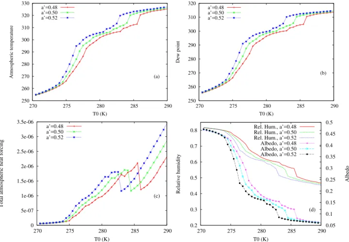
Fig. 2.Mean state as a function ofT0 for different values ofa′and withD=1.0 andT3=10 K, for(a)the atmospheric temperature,(b)the dew point,(c)the heat forcing (Eq. A8), and(d)the relative humidity and the albedo.
of T0 which is highly variable depending on the range of
T0 values considered. In particular for large values ofT0, a large jump is found in the diagram reflecting a drastic change of dynamics, as indicated also by the drastic decrease of the total atmospheric heat forcing shown in Fig. 2c. It is also worth noting that by increasing the parameter a′, a global shift of the curves toward smaller values ofT0 is found. In other word, for a specific value of the external forcingT0, the increase ofa′implies an increase of atmospheric temper-ature and dew point, and the albedo and relative humidity are decreasing. Note that this feature, specific to the present ide-alized model, could be different in other models for which cloud feedbacks and atmospheric absorption are more com-plicated.
Let us now look at the dynamical instability of this sys-tem (e.g. Kalnay, 2003). The Lyapunov exponents have been computed through a simple algorithm based on the (nonlin-ear) evolution of a set of small amplitude orthogonal pertur-bations. Different amplitudes have been tested without sub-stantial differences.
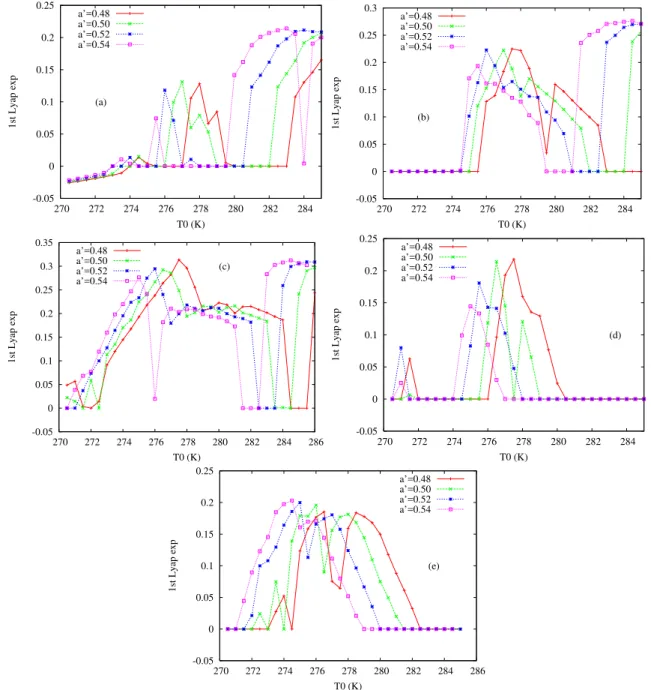
Figure 3 displays the dominant Lyapunov exponent as a function ofT0 for (a)T3=5 K and D=1, (b)T3=10 K andD=1, (c) T3=15 K and D=1, (d) T3=10 K and
D=0.1, (e) T3=15 K andD=0.1. Different curves are plotted for different values ofa′. In panel (a), Stable fixed points, (quasi-)periodic or chaotic solutions are found. In the other panels, there is no stable fixed points solutions for the range of values ofT0 explored.
Let us now be more specific by investigating the struc-ture of the bifurcation diagram forT3=10 K,a′=0.5 and
D=1 (panel b) which corresponds to the solution presented in Fig. 2. For small values ofT0 and for values ranging from 282 K to 284 K, the solution is (quasi-)periodic. For interme-diate values (between 275.5 K and 281.5 K) and the largest values explored (284.5 K and 285 K), the solution is chaotic. For these large values ofT0, mean temperature reaches very high values 315 to 320 K. These values are unrealistic for our midlatitude climate and in order to keep some resemblance with our climate atmosphere, we focus on smaller values of
-0.05 0 0.05 0.1 0.15 0.2 0.25
270 272 274 276 278 280 282 284
1st Lyap exp
T0 (K) (a)
a’=0.48 a’=0.50 a’=0.52 a’=0.54
-0.05 0 0.05 0.1 0.15 0.2 0.25 0.3
270 272 274 276 278 280 282 284
1st Lyap exp
T0 (K) (b)
a’=0.48 a’=0.50 a’=0.52 a’=0.54
-0.05 0 0.05 0.1 0.15 0.2 0.25 0.3 0.35
270 272 274 276 278 280 282 284 286
1st Lyap exp
T0 (K) (c) a’=0.48
a’=0.50 a’=0.52 a’=0.54
-0.05 0 0.05 0.1 0.15 0.2 0.25
270 272 274 276 278 280 282 284
1st Lyap exp
T0 (K)
(d) a’=0.48
a’=0.50 a’=0.52 a’=0.54
-0.05 0 0.05 0.1 0.15 0.2 0.25
270 272 274 276 278 280 282 284 286
1st Lyap exp
T0 (K)
(e) a’=0.48 a’=0.50 a’=0.52 a’=0.54
Fig. 3.Dominant Lyapunov exponent as a function ofT0 for different values ofa′, for(a)T3=5 K andD=1.0,(b)T3=10 K andD=1.0, (c)T3=15 K andD=1.0,(d)T3=10 K andD=0.1 and(e)T3=15 K andD=0.1.
(see panel c). When the volume of the Ocean is increased (D=0.1, panels d and e), a reduction of these maximum val-ues is experienced. The effect of increasinga′ is mainly to displace the whole Lyapunov diagram toward smaller values ofT0. This suggests that depending on the actual value of
T0, the system can experience either an increase or decrease of short term predictability as a function of the increase ofa′. 3.2.2 Post-processing
The central question of the present work is to know whether post-processing techniques can be used, after a climate change. In order to investigate this aspect, we first introduce
a model error in the system affecting its climate. Model er-rors are present in the various parameterizations used in at-mospheric or climate models, but in order to keep things sim-ple, we just introduce an error in the estimate of the coupling coefficientkbetween the Ocean and the Atmosphere. The actual value ofkis 0.015 and we fix for most of the experi-ments presented below a value for the model tok=0.014, so just a few percent errors.
-8 -7 -6 -5 -4 -3 -2 -1 0
270 272 274 276 278 280 282 284 286 288 290
Mean atmospheric temperature difference
T0 (K)
(a) D=1.0, T3=10 K
a’=0.48 a’=0.50 a’=0.52
-7 -6 -5 -4 -3 -2 -1 0 1 2
270 272 274 276 278 280 282 284 286 288 290
Mean atmospheric temperature difference
T0 (K)
(b) D=0.1, T3=10 K
a’=0.48 a’=0.50 a’=0.52
-10 -8 -6 -4 -2 0 2
270 272 274 276 278 280 282 284 286 288 290
Mean atmospheric temperature difference
T0 (K)
(c) D=1.0, T3=15 K
a’=0.48 a’=0.50 a’=0.52
-6 -5 -4 -3 -2 -1 0 1 2 3 4
270 272 274 276 278 280 282 284 286 288 290
Mean atmospheric temperature difference
T0 (K)
(d) D=1.0, T3=10 K
a’=0.48 a’=0.50 a’=0.52
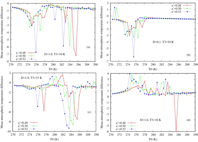
Fig. 4. (a)Temperature bias between the reference system withk=0.015 and the model version withk=0.014 for different values ofa′, and withD=1.0 andT3=10 K;(b)as in(a)but withD=0.1 andT3=10 K;(c)as in(a)but withD=1.0 andT3=15 K; as in(a)but with a model version withk=0.016, and withD=1.0 andT3=10 K.
the model structure. This specific choice has an impact on the post-processing correction for short times because the larger is the initial condition error, the smaller is the po-tential correction of the method (see Vannitsem and Nicolis, 2008). However it does not qualitatively modify the conclu-sions drawn below.
The climate mean
Let us first consider the case where only the bias between reality and model is corrected as it is usually the case for cli-mate projections. Figure 4 displays the difference between the climatological averages of the air temperature for dif-ferent parameter settings and difdif-ferent values ofa′, reality-model. The difference is strongly dependent on the value of
T0, from just a few tenth of degrees up to 7 degrees. Once this quantity is known, one can correct the forecast for the mean temperature. Let us now assume that the system is ex-periencing a climate change through an increase of the pa-rametera′. In this case the mean difference (the system-atic bias of the model) can be very different as illustrated in Fig. 4. For instance if one focuses on the case where
T0=277 K,T3=10 K andD=1.0, the difference can pass
from about−1.5 degrees fora′=0.48 to−3.5 fora′=0.50 and back to −1 for a′=0.52. This of course has strong influences when one wants to infer the absolute values of the change in mean temperature expected in the future. In the present example, one would overestimate the mean tem-perature after climate change by about 2 degrees (fora′ go-ing from 0.48 to 0.50), even if we know exactly howa′has changed. For other parameter values, the effect can be much milder but sometimes it can be very dramatic like when the system is close to a qualitative change of dynamics as for
T0=283.5 K or 276 K (up to 6 degrees) in panel (a), or even more as in panel (c) and can sometimes even change sign (panels b and c). Note that there is almost no change of the biases when the dynamics becomes (quasi-)periodic (see Fig. 3). For larger value of the model parameterk (0.016 in panel d) a similar picture holds, but the bias is most of the time of the opposite sign to the ones corresponding to
k=0.014.
(Solomon et al., 2007). In other words, the impact of model errors cannot be simply considered as a purely constant sys-tematic additive term. This introduces a further (probably rather large) uncertainty on the possible future outcomes of the climate system, associated with the presence of model errors.
Finally, one can wonder whether developing an ensemble scheme based on a set of forecasts using different parame-ters (as discussed for instance in Stainforth et al., 2007) is worth doing in order to evaluate the range of possible out-comes. 100 runs are performed with different values of k
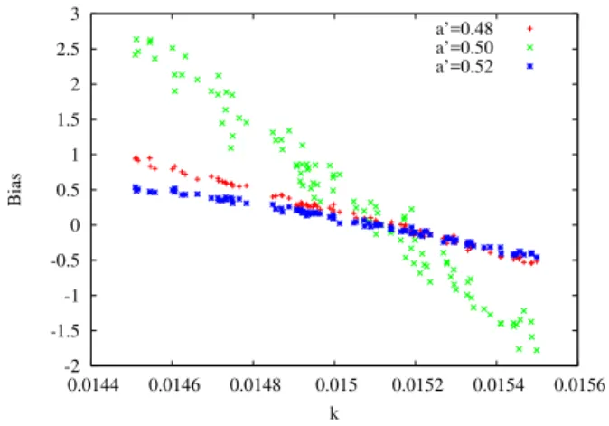
ranging from[0.0145,0.0155]. The reference value is cho-sen as one model coming from this ensemble (k=0.01511). The mean temperature is computed for this set of models and for three different values ofa′. The mean temperature biases are plotted as a function ofk in Fig. 5. First the range of possible biases for this ensemble of model runs differs con-siderably from one value ofa′ to another, and there is no clear dependence of this quantity as a function ofa′. This in-dicates that the actual uncertainty of the model biases cannot be straightforwardly transposed to another value ofa′(or in other words for different absorption forcings). But what is interesting to mention is that there is an almost linear depen-dence of the bias as a function ofk, suggesting that the best models are the ones having a value ofkclose to the actual one, whatever is the value ofa′. This supports the usefulness of classifying the quality of the models under the current cli-mate conditions as in Giorgi and Mearns (2003), as a con-fidence in their climate projections. But still one should be cautious because these results have been obtained for a small range of uncertainty ofkand assuming that the model error is only associated with the error of a parameter. Other sources of model errors can play an even more important role, like processes not represented in the model (referred to asmodel inadequacyin Stainforth et al., 2007). These could change the conclusions but the analysis of this aspect is beyond the scope of the present work and is worth performing in a more complicate model.
Linear post-processing of forecasts
Long term projections on centennial or millennial time scales are one aspect of climate prospective. Another domain of very active research is to try to perform some climate fore-casts on shorter time scales, from seasons to decadal time scales. These forecasts are also affected by model errors and furthermore are subject to slow changes of the climate forc-ings. Let us now focus on a more “sophisticated” (linear) post-processing technique, already discussed in Sect. 2, aim-ing at correctaim-ing forecasts. Again as in the previous section, one assumes that the climate change is simply represented by an increase ofa′without any additional transient dynam-ics. The training of the post-processing technique is first per-formed on forecasts obtained with one value ofa′and then applied and verified on a second set of forecasts obtained
-2 -1.5 -1 -0.5 0 0.5 1 1.5 2 2.5 3
0.0144 0.0146 0.0148 0.015 0.0152 0.0154 0.0156
Bias
k
a’=0.48 a’=0.50 a’=0.52
Fig. 5. Mean temperature bias for different values ofkanda′. The reference value ofk is 0.01511, for eacha′. D=1.0,T3=10 K andT0=277 K.
with another value of a′. The number of forecasts for the training and verification phases is fixed to 5000. The regres-sion is performed for each lead time of the forecast and at each grid point of the system grid.
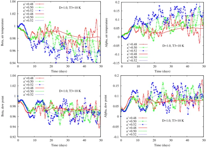
Figure 6 displays the time variation of the parameterβ(t )
andα(t )for the air temperature and dew point for
parame-ter valuesD=1.0,T0=277 K andT3=10 K and for one specific location of the central row of the grid of this coupled system. Three different parameter valuesa′ are displayed. The lines without symbols represent a running average of the parameters starting after about 15 days. Two time scales should be distinguished, before and after about 10 days. For the atmospheric temperature at short time scales, the param-eters are close fora′=0.48 and 0.50, while fora′=0.52 it varies in an opposite direction. For dew point, the picture is slightly different where the variations of the parameters are closer to each other for short time scales. For longer time scales, the variability of the parameters is pronounced and the running mean values (lines without symbols) are sub-stantially different for the different parameter valuesa′. This variability is associated with the rather “small” number of forecasts used for the training.
0.94 0.96 0.98 1 1.02 1.04
0 10 20 30 40 50
Beta, air temperature
Time (days) D=1.0, T3=10 K a’=0.48
a’=0.50 a’=0.52 a’=0.48 a’=0.50 a’=0.52
-0.15 -0.1 -0.05 0 0.05 0.1 0.15 0.2
0 10 20 30 40 50
Alpha, air temperature
Time (days) D=1.0, T3=10 K a’=0.48
a’=0.50 a’=0.52 a’=0.48 a’=0.50 a’=0.52
0.92 0.94 0.96 0.98 1 1.02 1.04
0 10 20 30 40 50
Beta, dew point
Time (days) D=1.0, T3=10 K a’=0.48
a’=0.50 a’=0.52 a’=0.48 a’=0.50 a’=0.52
-0.1 -0.05 0 0.05 0.1 0.15 0.2
0 10 20 30 40 50
Alpha, dew point
Time (days) D=1.0, T3=10 K a’=0.48
a’=0.50 a’=0.52 a’=0.48 a’=0.50 a’=0.52
Fig. 6. Variations of the parameterαandβat a function of lead time for different values ofa′at one specific location of the grid (one grid point in the middle row). Panels(a)and(b)for air temperature and(c)and(d)for dew point.D=1.0 andT3=10 K. The continuous lines without symbols are running averages starting after 15 days in order to evaluate the average level values of the parameters at long lead times.
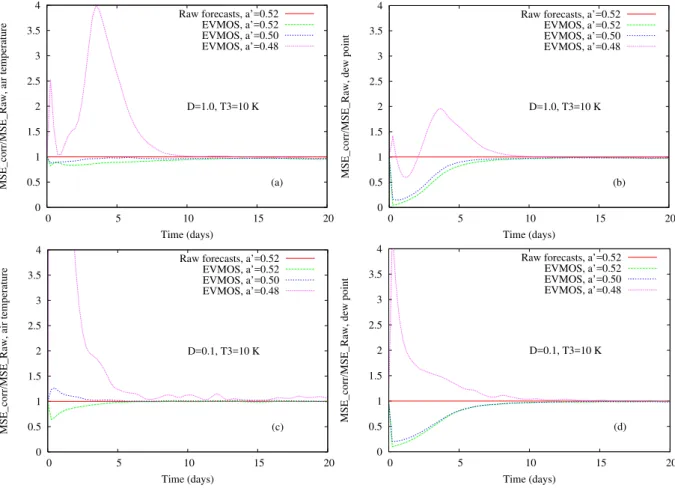
Figure 8 displays the variations of the mean square error ratio for post-processing trained with different values ofa′
and applied on a set of forecasts produced ata′=0.52. The lead time is fixed to 5 days and two different values of D
are considered, namely 1.0 and 0.1. This results indicate that the traditional post-processing approach can be useful but in some restricted situations, for which the dynamics does not vary much between the training and the verification phases. This corroborates the results of Sect. 2. Moreover, the vari-ations of the quality of post-processing display a complicate nonlinear dependence, as a function of the difference be-tween the values ofa′used for verification and for training.
4 Conclusions
Statistical post-processing is a common approach to correct weather and climate forecasts, as well as climate projections. The main assumption behind these approaches is the station-arity of the correction parameters allowing for an application of the techniques for new runs or forecasts. Under climate change, this hypothesis is not realistic, as it has been amply
demonstrated in the present paper. In particular biases can display linear or non-linear variations depending on many aspects, the nature of the underlying dynamics, the source of model errors, the intensity (velocity of change) of the forcing scenario and its uncertainty. These features are system spe-cific, increasing considerably the difficulty in assessing the quality of future forecasts or projections, and their potential corrections.
This analysis has been performed here in the context of very simple systems. A natural extension will be the in-vestigation of an intermediate order climate model in the same spirit in the presence of realistic model errors. This analysis could provide a more quantitative information on the variations of biases and post-processing parameters, that could guide future estimates of the uncertainties of climate forecasts or projections and the development of correction schemes based on non-stationary coefficients.
0 0.5 1 1.5 2 2.5 3 3.5 4
0 5 10 15 20
MSE_corr/MSE_Raw, air temperature
Time (days)
(a) D=1.0, T3=10 K Raw forecasts, a’=0.52
EVMOS, a’=0.52 EVMOS, a’=0.50 EVMOS, a’=0.48
0 0.5 1 1.5 2 2.5 3 3.5 4
0 5 10 15 20
MSE_corr/MSE_Raw, dew point
Time (days)
(b) D=1.0, T3=10 K Raw forecasts, a’=0.52
EVMOS, a’=0.52 EVMOS, a’=0.50 EVMOS, a’=0.48
0 0.5 1 1.5 2 2.5 3 3.5 4
0 5 10 15 20
MSE_corr/MSE_Raw, air temperature
Time (days)
(c) D=0.1, T3=10 K Raw forecasts, a’=0.52
EVMOS, a’=0.52 EVMOS, a’=0.50 EVMOS, a’=0.48
0 0.5 1 1.5 2 2.5 3 3.5 4
0 5 10 15 20
MSE_corr/MSE_Raw, dew point
Time (days)
(d) D=0.1, T3=10 K Raw forecasts, a’=0.52
EVMOS, a’=0.52 EVMOS, a’=0.50 EVMOS, a’=0.48
Fig. 7. Ratio of the Mean Square Error (MSE) of the corrected forecasts and the MSE of the raw forecasts for a value ofa′=0.52. The MSE is evaluated over the whole grid. The different curves correspond to the use of post-processing schemes trained using different values ofa′.D=1.0 andT3=10 K.
0.6 0.8 1 1.2 1.4 1.6 1.8 2 2.2 2.4 2.6 2.8
0.48 0.485 0.49 0.495 0.5 0.505 0.51 0.515 0.52
MSE_corr/MSE_raw
a’
T0=277 K, T3=10 K Air temperature, D=1.0 Dew point, D=1.0 Air temperature, D=0.1 Dew point, D=0.1
Fig. 8. Ratio of the Mean Square Error (MSE) of the corrected forecasts and the MSE of the raw forecasts for a value ofa′=0.52, as a function of the value ofa′ used for the training of the post-processing scheme. The MSE is evaluated over the whole grid and the lead time is fixed to 5 days.
touched upon by performing a few runs with different pa-rameter values reflecting the model uncertainty. In this case the result suggests that the closest is the model parameter value from the true value, the smaller is the bias. In other words, the ranking of the quality of the models seems to be more robust than the amplitude of the bias. This could jus-tify the usefulness of some statistical approaches (e.g. Giorgi and Mearns, 2003; Duan and Phillips, 2010 and reference therein) providing a larger weight to projections generated by the models matching best the current observations. Weigel et al. (2010) however pointed out the difficulty in finding cor-rect weights for each model of the ensemble, that could lead to worse results than equal weighting. This clearly points out the necessecity for a thorough analysis of these approaches in simple dynamical systems, in a similar vein as in the present work.
Appendix A
The low-order moist general circulation model
The model developed by Lorenz (1984) is a coupled Ocean-Atmosphere model, whose atmosphere is composed of a mixture of dry air and water into two possible phases, vapor or liquid. The Ocean is just a heat bath at which the atmo-sphere is coupled and with which it exchanges water and heat through simple parameterizations. The domain is periodic in the west-east direction and bounded on the North and South by frictionless vertical walls. The atmosphere is described as a baroclinic dynamics defined on aβ plane. The exter-nal driving force is the incoming solar radiation. The basic prognostic equations are: the vorticity equation,
∂∇2ψ
∂t +J (ψ,∇
2ψ ) +β∂ψ
∂x = −f∇
2ξ
+F (A1)
whereψ,ξ andF are the streamfunction, the velocity po-tential and the curl of the viscous drag, respectively. The op-eratorJ is the Jacobian,f andβ are the coriolis parameter defined for the midlatitudes and its first derivative, respec-tively; The thermodynamic equation
d(cpT+Lv)
dt =
RT ω
p +H (A2)
whereT,v,ωandH are the air temperature, the water va-por mixing ratio, the vertical velocity in pressure coordinates and the atmospheric diabatic heating per unit mass, respec-tively, andLandcp are the latent heat of condensation and the specific heat of air at constant pressure; the water content equation,
dw
dt =G (A3)
wherewandGare the total water mixing ratio and the gain or loss of water by evaporation or precipitation, respectively; and the oceanic thermodynamic equation,
dcS
dt =E (A4)
whereSandEare the oceanic temperature and the oceanic heating per unit mass, respectively. The coefficientcis the specific heat of water. These prognostic equations are com-plemented by the diagnostic continuity and thermal wind equations. Note that the total water mixing ratio is itself transformed into a dew point temperature through the diag-nostic relation,
w=c′Wµ/p (A5)
whereµis a constant fixed toL/RwTs≈20, derived through
a simplification of the Clausius-Clapeyron equation. Equa-tion (A3) is replaced by an equaEqua-tion for the dew point tem-perature.
This system of equations is then simplified through a two-layer vertical discretization for which the streamfunction is defined at two levels and temperature (air or dew point) at an intermediate level, and in the horizontal direction by focusing only on the largest modes. This approximation reads
X=
6 X
n=0
Xn8n
where
80=1
83j−2=2sin(jy)cos(2x)
83j−1=2sin(jy)sin(2x)
83j=
√
2cos(jy)
forj=1,2. All the variables are adimensionalized, with the charactristic scales fixed tof−1=3 h, L=1830 km, p0=
1000 mb, and the unit of temperature is equal to 100 K. Lorenz (1984) also has proposed a pseudo-specral method to evaluate the sources and sinks terms and the nonlinear terms appearing in the equations. The grid developed by Lorenz is composed of 9 grid points. All the parameters are fixed as in Lorenz (1984), except the lapse rate fixed to 0.215 as in Nese et al. (1996). The integration time step is fixed to 0.02 time units.
The vertically averaged forcings are given by the relations
F= −k∇2ψ (A6)
F= −k′∇2T (A7)
H= −k{cp(T−S)+L(v−s)} +HR (A8)
G= −k(v−s)−(lν/λ)(w−v) (A9)
E= − p0
p1−p0
k{cp(S−T )+L(s−v)} +ER (A10)
wheres is the saturation mixing ratio at temperatureS and mean sea level pressure p0. p1 is the pressure at bottom
of oceanic layer. k is the coupling coefficient between the ocean and the atmosphere. Another damping term (A7) with coefficientk′ is reducing the shear between the two levels. 1/ lis a damping time scale corresponding to the half life of clouds (water delivered as rain). A new constant containing information on the volume of the oceanic layer is defined as
HR=(σ g/p0)v′a′′(S4−T′′4−T′4) (A11)
ER=(σ g/(p1−p0))(−S4+v′a′′T′′4−(1−v′a)T∗4) (A12)
where
v′a′′=v′(a+(1−a)a′) (A13) accounts for the fraction of heat effectively absorbed by the atmosphere where 1−a′ is the fraction of longwave radia-tion that will go out the atmosphere without absorpradia-tion. Note that in the original discussion of Lorenz (1984),a′was con-sidered as the part transmitted toward space, but it cannot coincide with the effective fraction of heat absorbed by the atmosphere, Eq. (A13), except in the case ofa′=0.5 which is precisely the value chosen by E. Lorenz. σ is the Stefan constant,T′andT′′are temperatures at which the cloud-free portion of the atmosphere is radiated upward and downward, respectively, andv′=v/(v+vs)wherevsis a reference
wa-ter vapor mixing ratio.
Finally the solar forcing entering in the termERdepends
on 2 Fourier coefficients,
T∗ =T080+T383
In this idealized coupled ocean-atmosphere system, one can wonder how one can simulate a climate change associ-ated with the variations or atmospheric absorption. The an-swer can be simply by modifying the net absorption of long-wave radiations coming from the ocean by the atmosphere. So we will simply focus on variations of the parametera′, appearing in Eq. (A13). This parameter will be modified in such a way that the mean air temperature difference reaches a few degrees (temperature differences expected in a climate change).
Acknowledgements. We are indebted to Aim´e Fournier for having
provided the original code of the Lorenz (1984) model, as well as for his help in understanding its features. This work has benefited from discussions with C. Nicolis, from an inspiring presentation made by L. Smith, and from the comments of the anonymous reviewers. This work is partly supported by the Belgian Federal Science Policy Office under contracts SD/CA/04A and MO/34/020.
Edited by: W. Hsieh
Reviewed by: two anonymous referees
References
Benestad, R. E., Hanssen-Bauer, I., and Chen, D.: Empirical-statistical downscaling, World Scientific, Singapore, 215 pp., 2008.
Berner, J., Doblas-Reyes, F. J., Palmer, T. N., Schutts, G., and Weisheimer, A.: Impact of a quasi-stochastic cellular automaton backscatter scheme on the systematic error and seasonal predic-tion skill of a global climate model, Phil. Trans. R. Soc. A, 366, 2561–2579, 2008.
Buser, Ch. M., K¨unsch, H. R., L¨uthi, D., Wild, M., and Sch¨ar, C.: Bayesian multi-model projection of climate: bias assumptions and interannual variability, Clim. Dynam., 33, 849–868, 2009. Christensen, J. H., Boberg, F., Christensen, O. B., and Lucas-Picher,
Ph.: On the need for bias correction of regional climate change of temperature and precipitation, Geophys. Res. Lett., 35, L20709, doi:10.1029/2008GL035694, 2008.
Dijkstra, H.: Nonlinear Physical Oceanography, Springer Dor-drecht, New York, 532 pp., 2005.
Dijkstra, H. and Ghil, M.: Low-frequency variability of the large scale ocean circulation: A dynamical system approach, Rev. Geophys., 43, RG3002, doi:10.1029/2002RG000122, 2005. Duan, Q. and Phillips, Th. J.: Bayesian estimation of local signal
and noise in multimodel simulations of climate change, J. Geo-phys. Res., 115, D18123, doi:10.1029/2009JD013654, 2010. Gardiner, C. W.: Handbook of stochastic methods, Springer-Verlag,
New-York, 442 pp., 1985.
Giorgi, F. and Mearns, L. O.: Probability of regional climate change based on the reliability ensemble averaging (REA) method, Geo-phys. Res. Lett., 30, 1629–1632, 2003.
Glahn, B., Peroutka, M., Wiedenfeld, J., Wagner, J., Zylstra, G., Schuknecht, B., and Jackson, B.: MOS uncertainty estimates in an ensemble framework, Mon. Weather Rev., 137, 246–268, 2009.
Johnson, Ch. and Swinbank, R.: Medium-range multimodel ensem-ble combination and calibration, Q. J. R. Meteorol. Soc., 135, 777–794, 2009.
Kalnay, E.: Atmospheric modeling, data assimilation, and pre-dictability, Cambridge University Press, 341 pp., 2003. Knutti, R., Allen, M. R., Friedlingstein, P., Gregory, J. M., Hegerl,
G. C., Meehl, G. A., Meinshausen, M., Murphy, J. M., Plattner, G.-K., Raper, S. C. B., Stocker, T. F., Stott, P. A., Teng, H., and Wigley, T. M. L.: A review of uncertainties in global temperature projections over the twenty-first century, J. Climate, 21, 2651– 2663, 2008.
Lorenz, E. N.: Formulation of a low-order model of a moist general circulation, J. Atmos. Sci., 41, 1933–1945, 1984.
Nese, J. M., Miller, A. J., and Dutton, J. A.: The nature of predictability enhancement in a low order Ocean-Atmosphere model, J. Climate, 9, 2167–2172, 1996.
Nicolis, C.: Transient climatic response to increasingCO2 concen-tration: some dynamical scenarios, Tellus, 40A, 50–60, 1988. Nicolis, C. and Nicolis, G.: Passage through a barrier with a slowly
increasing control parameter, Phys. Rev. E, 62, 197–203, 2000. Schmith, T.: Stationarity of regression relationships: Application to
empirical downscaling, J. Climate, 21, 4529–4537, 2008. Solomon, S., Quin, D., Manning, M., Chen, Z., Marquis, M.,
Av-eryt, K. B., Tignor, M., Miller, H. L. (Eds): Climate Change 2007: The physical Science Basis. Contribution of Working Group I to the Fourth Assessment Report of the Intergouvern-mental Panel on Climate Change, Cambridge University Press, Cambridge, United Kingdom and New York, NY, USA, 2007. Stainforth, D. A., Allen, M. R., Tredger, E. R., and Smith, L. A.:
Confidence, uncertainty and decision-support relevance in cli-mate predictions, Phil. Trans., R. Soc., 365, 2145–2161, 2007. Vannitsem, S.: A unified linear model output statistics scheme for
both deterministic and ensemble forecasts, Q. J. R. Meteorol. Soc., 135, 1801–1815, 2009.
patterns in a T21L3 quasigeostrophic model, J. Atmos. Sci., 54, 347–361, 1997.
Vannitsem, S. and Nicolis, C.: Dynamical properties of model out-put statistics forecasts, Mon. Weather Rev., 136, 405–419, 2008.
Van Schaeybroeck, B. and Vannitsem, S.: Post-processing through linear regression, Nonlin. Processes Geophys., 18, 147–160, doi:10.5194/npg-18-147-2011, 2011.