Strategic noise mapping with GIS for the Universitat Jaume I Smart Campus: Best Methodology Practices

(1)

i

Strategic noise mapping with GIS for the Universitat Jaume I

Smart Campus: Best Methodology Practices

(2)

ii

Strategic noise mapping with GIS for the Universitat Jaume I

Smart Campus: Best Methodology Practices

(3)

iii

Strategic noise mapping with GIS for the Universitat Jaume I Smart Campus:

Best methodology practices

by Sarah Eason saraheasongis@gmail.com Institute of New Imaging Systems,

Universitat Jaume I, Castellon, Spain

Dissertation supervised by

Michael Gould, PhD Global Education Manager, ESRI

Professor of Information Systems, Institute of New Imaging Systems, Universitat Jaume I,

Castellon, Spain

Dissertation co-supervised by

Joaquin Huerta, PhD

Professor, Institute of New Imaging Systems, Universitat Jaume I,

Castellon, Spain

Marco Pinho, PhD

Instituto Superior de Estatica e Gestau de Informacao Universidade NOVA de Lisboa

Lisbon, Portugal

(4)

iv

ACKNOWLEDGEMENTS

I would like to thank Dr. Michael Gould for supervising my thesis and Dr. Joaquin Huerta and Dr. Marco Painho for co-supervising. I am privileged to have participated in the Master of Science in Geospatial Technologies. I thank the Erasmus Mundus Association, the Institute for New Imaging Technologies (INIT), Universitat Jaume I (UJI),Castellon, Spain, the Institute for Geoinformatics (IFGI), University of Munster, Germany and the Institute Superior of Statistics and Information (ISEGI), Lisbon, Portugal for providing this wonderful opportunity and all the rich experiences I have had during my time in Europe.

I would like to thank Dr. Jorge Mateu for his guidance with the statistical methodology used in this research, and Andres Munoz for his guidance with ArcGIS Modelbuilder and other GIS issues.

I also thank Luis Rodriguez a for developing the Noise Battle application and providing assistance with it and other related elements throughout my research. He was always willing and able to provide support in the programming area. I am grateful to Ana Sanchis Huerta for providing the initial idea for this thesis topic. I thank my fellow classmates for their friendship and camaraderie.

I would also like to thank ReMa Medio Ambiente, S.L. for sharing their data to make my research possible, and especially to Ricardo Blasco Troncho, Joaquin Gargallo Saura, with whom I conducted my fieldwork.

I extend my gratitude to sound engineer Bill Stevens in Texas, who kindly provided me with acoustic theory textbooks to which I would not have otherwise had access, and which made my research possible.

I would also like to thank my parents, Richard and Lynn Eason, for their constant support, emotionally, mentally, morally, financially and physically. They cheered me on and were willing at all hours of the night to review my work and discuss and revise its progress all along the way. My father was invaluable in his ability to coach me into an understanding of acoustic principles.

(5)

v

Strategic noise mapping with GIS for the Universitat Jaume I Smart Campus:

Best methodology practices

ABSTRACT

Noise is a type of pollution often overlooked in conversations about pollution, which usually center on air, water and waste management. However, it has not been missed by decision makers in the European Union (EU). There are laws to keep noise levels down, and schools are a target specifically mentioned in the European Environmental Noise Directive (END). Strategic noise mapping can identify problem areas and help evaluate situations. This thesis project explores and compares various approaches in an attempt to offer useful information to the noise mapping field based on the results of the analysis. The

measurements used commonly in studies are taken by professionals using professional equipment. Either teams physically enter the environment to manually take measurements or they collect data wirelessly from fixed sensors. Both of these methods are expensive due to the manpower or equipment. In addition, these methods are limited in the number of measurements in space and time that they can represent. One option is to use citizens with smart phones to record noise measurements. Involving the public to gather information is commonly called crowdsourcing, Volunteered Geographic Information (VGI) or Public Participatory GIS (PPGIS). Three applications for Android smart phones were tested and compared to a certified, calibrated professional sound level meter. Also, mapping noise by taking sample noise

measurements without also mapping noise sources may not provide the full picture. The second objective of this thesis was to apply sound attenuation and combination rules in ArcGIS to create a noise source map and compare the results to the common spatial interpolation methods. The comparisons of smart phone measurements with the professional sound level measurements revealed that they are not comparable quality. Each ANOVA and t-Test revealed statistically significant differences. This is mostly attributed to the phone’s hardware, which varies between mobile device models and versions. The geostatistical interpolation tools delivered noise maps which had similar accuracy rates for predicting measurement points according to the cross validation methods used. The best (most accurate) prediction model was indeed the kriging method. The author successfully applied sound attenuation equations to create a multiple noise source propagation and combination interpolation toolset in ArcGIS. This can be used for an infinite number of noise sources. The fit of the actual measurement points in the noise source attenuation noise map was very similar although slightly higher than that of to the geostatistical methods

KEYWORDS

(6)

vi ACRONYMS

2D two-dimensional

ANOVA Analysis of Variance

ArcGIS Trademark name of ESRI GIS software

CESVA CESVA instruments, S.L. (private company)

dB decibel

dB(A) A-weighted decibel

den day-evening-night

END European Noise Directive

ESRI Environmental Systems Research Institute

EU European Union

GIS Geographic Information Systems or Science

GPS Global Positioning System

IDW Inverse Distance Weighted

LeqT Mean decibel level for five minute period

PPGIS public participatory GIS

RBF Radial Based Function

ReMa ReMa Medio Ambiente, S.L. (private company)

UJI Universitat Jaume I

(7)

(8)

(9)

(10)

(11)

(12)

(13)

1

1. Introduction

1.1 Rationale

The Universitat Jaume I (UJI) in Castellon, Spain is in the process of becoming a Smart Campus. New technologies are being used to bring the UJI to the forefront of sustainability. With a view to improve resource management, alternative energies are being explored and conservation methods investigated. Masters students from Madrid and the Erasmus Mundus visiting scholar have joined with the team at UJI to start the creation of a two-dimensional (2D) campus map using the Environmental Systems Research Institute (ESRI) Campus Basemap Template. This project has a wide scope of opportunities to use the basemap and the tools of Geographic Information Systems (GIS). Topics range from energy consumption to facilities management to green building and sustainability. Crowdsourcing is increasing in popularity as a new way to collect data from the public, including health and allergy information, behavior monitoring and incident and problem reporting services and maintenance requests. Mobile applications for smart phones such as place finders and navigation routing for both vehicles and pedestrians can be integrated with the campus basemap. Another interesting and important application is pollution control. Noise is a type of pollution often overlooked in conversations about pollution, which usually center on air, water and waste management. However, it has not been missed by decision makers in the European Union (EU). There are laws to keep noise levels down, and schools are a target specifically mentioned in the European Environmental Noise Directive (END). Strategic noise mapping can identify problem areas and help evaluate situations. Garcia Marti et al. suggest a few approaches to noise mapping. One is to apply “physical noise propagation laws to well-known noise sources,” another is to interpolate data from a “network of sensor devices,” and a third is to build a database from data collected through the “direct participation of citizenship” (Garcia Marti 2012). This thesis project aims to explore and compare these approaches and offer useful information to the noise mapping field based on the results of the analysis.

1.2 Background

(14)

2

1.3 Motivation

Since 2008, more than half of the world’s population lives in urban areas. Urban areas are polluted by many sources and noise is one of them. Noise at night above 45 decibels is considered a sleep disturbance. Noise can be merely annoying, but repeated or continuous noise throughout the day can be harmful to the health of people young and old. The Columbia Encyclopedia reports the following:

Apart from hearing loss, such noise can cause lack of sleep, irritability, heartburn, indigestion, ulcers, high blood pressure, and possibly heart disease. One burst of noise, as from a passing truck, is known to alter endocrine, neurological, and cardiovascular functions in many individuals; prolonged or frequent exposure to such noise tends to make the physiological disturbances chronic. In addition, noise-induced stress creates severe tension in daily living and contributes to mental illness (Columbia 2011).

A 2006 European Commission Green Paper claims noise is “one of the main local environmental problems in Europe and the source of an increasing number of complaints from the public” (European 2006). The paper aims to encourage discussion and solutions to the problem and encourages the study of noise pollution by all member states.

1.4 Problem Statement

1.4.1 Can crowdsourced noise measurements help provide useful information to noise mapping?

The measurements used commonly in studies are taken by professionals using professional equipment. Either teams physically enter the environment to manually take measurements or they collect data wirelessly from fixed sensors. Both of these methods are expensive due to the manpower or equipment. In addition, these methods are limited in the number of measurements in space and time that they can represent. Garcia Marti et al. propose that “in this context, it is important to consider a different way for data collection with a high temporal and spatial noise data resolution and with a low deploying cost.” One option is to use citizens with smart phones to record noise measurements. Involving the public to gather information is commonly called crowdsourcing, volunteered geographic information (VGI) or public participatory GIS (PPGIS). It is certainly a cheaper route, although it has not been proven to be a completely reliable replacement.

Three applications for Android smart phones will be tested and compared to a professional sound level meter. Will these applications report similar noise measurements? If not, are the differences consistent enough to apply a rule to the measurements to normalize them? For example, will adding or subtracting five decibels to all the smart phone measurements bring them to the same level as the professional meter’s measurements? Furthermore, if serious errors exist, what is the source - the software, the hardware, or the human?

1.4.2 Which is the best methodology to make a noise map?

(15)

3

packages are lacking for many places and simpler approaches must be used. A common choice is to simply interpolate between sample noise measurement points and overlay the resulting raster on a map.

Creating a noise map seems at first like any other exercise in interpolation. One could take sample measurements at a variety of locations and use one of the ArcGIS tools to interpolate the unknown values between the known ones. However, would this be an accurate representation of reality? This question is important, first, because the decibel scale is logarithmic, not linear. This is due to the fact that the range of sound levels is so wide, and that the logarithmic scale corresponds to the perception by the human ear of the relative loudness of different sounds (Oliviera 1999). Each increase of ten decibels is a doubling of the subjective loudness. For example, 80 decibels is twice as loud as 70; 90 is four times as loud; and 60 is only half as loud (Airport 2013). Therefore, in order to accurately interpolate sound measurements, one must understand and employ the rules of sound attenuation. Sound is a wave which travels through the air, losing energy as it moves outward in all directions. Attenuation is defined by the Princeton online dictionary as “weakening in force or intensity" (Princeton 2013). Furthermore, when combining the sound levels of multiple sources, one cannot simply add or average the decibel levels. There are rules for this as well. Do common interpolation methods properly account for this? Also, mapping noise by taking sample noise measurements without also mapping noise sources may not provide the full picture. The second objective of this thesis will be to apply these sound attenuation and combination rules in ArcGIS and compare the results to the common interpolation methods.

1.5 Scope

The study area is the UJI campus. The study area feature is simply a polygon drawn around the UJI campus and surrounding areas. Its dimensions, extending beyond the explicit bounding box defined by the extents of the campus, were chosen by the author to attempt to create a more realistic model. Since UJI does not exist in a vacuum, but instead in the midst of a bustling town full of traffic and just southwest of the large Autopista del Mediterrani, these surrounding noises must surely contribute to the noise on campus. Therefore, to accurately draw a noise map, these surrounding areas must be included in the model. Although the END specifies taking measurements for the daytime and nighttime, nighttime will be excluded for this study. The ReMa measurements stop at 22:00 and no testing is done past that time. There is a student residence in the southwest corner of the campus, but the ReMa noise mapping is focused on the setting as a school, not as a residential area.

2. Literature Review

2.1 Understanding Decibels

Decibel is a tenth of a bel, named for Alexander Graham Bell. A bel is the ratio of two sound intensities (I1 and I2). Decibels are the measure of unit defined to best approximate the way the human ear perceives sound, which is similar to a logarithmic curve. “This means simply that the response is approximately proportional to the logarithm of the stimulus. It is not directly proportional to the stimulus” (Wadsworth 1983).

(16)

4

(Wadsworth 1983)

Therefore the decibel is a ratio, not a quantity; it “does not tell how much but how many times one quantity exceeds another” (Wadsworth 1983). Furthermore, the multiplier goes from 10 to 20 when pressure is being represented instead of intensity, and the new equation follows:

(Wadsworth 1983)

Finally, there is a rule occurring from the mathematics which states that each time the distance from the source doubles, the there is a six decibel decrease. This is demonstrated below:

(Wadsworth 1983)

This understanding of sound and how it is perceived and measured should be taken into consideration when designing a noise map based on well-known noise sources rather than sample measurements.

(17)

5

2.2 Understanding Noise and Decibels

Table 1 below exemplifies familiar sounds and their corresponding decibel levels and effects.

(18)

6

It is important to remember how decibels relate to human perception of sound. Table 2 below describes a few of these relationships. A 10 decibel decrease is perceived as half as loud, and a decrease of 20 decibels as one quarter as loud.

Table 2: Perceptions Chart (Decibel 2012)

Table 3 shows the (USA) Occupational Safety and Health Administration rules to limit sounds which people should be exposed to. Levels beyond this are generally accepted to be harmful to human health (Decibel 2012).

Table 3: OSHA Chart (Decibel 2012)

Table 4 shows the (USA) National Institute for Occupational Safety and Health rules to limit sounds which people should be exposed to. There is not much difference between the two charts (Decibel 2012).

(19)

7

Table 5 shows the World Health Organization guidelines for noise levels (Future 1996). Note especially that the outdoor limit for schools is 55 decibels, and no nighttime limits are defined, although some universities have residences on their campuses. This is in keeping with ReMa’s noise measurements only recording daytime values.

Table 5: WHO Chart (Future 1996)

(20)

8

2.3 Noise Data Collection Technique

2.3.1 Sampling Grids and Wireless Sensor Networks

There are many elements in the process of noise mapping, and many choices to be made at each step. The measurement collection scheme must be devised to reflect different times of day and different parts of the study area. A regular grid is a common plan and can be drawn manually or selected by a software program, but some of the points may fall inside a building footprint. The choices are to take the measurement from the roof in the correct location, to move the location to the nearest possible spot on the ground or to eliminate the point altogether (Arana 2009). An additional method is to select major intersections instead of trying to use a geometrical grid (Yilmaz 2006).

Another element to consider is the source. Noise sources can be mapped as points or lines. While individual vehicles could be represented as points, traffic noise is generally modeled as a line representing the roadway. It is also possible to represent traffic as “a line of point sources” (De Muer 2003). Features such as air conditioning units, construction sites and other machinery usage can be modeled as points. Arana suggests that although lines can be more reliable for precise knowledge, a true evaluation of the sources requires using both points and line sources (Arana 2009). Another approach is to use an image of the study area and define the pixels of a noise source as a line, thereby creating a line source map from a point source map (Yilmaz 2006).

A study in Nigeria used a professional sound level meter to collect data, but instead of making noise maps, they quantified the areas according to areas in violation of allowed sound levels and returned results in the form of charts and action plans for various land use settings. “The selected areas of study are commercial centers, road junctions/busy roads, passenger loading parks, and high-density and low-density residential areas. The road junctions had the highest noise pollution levels, followed by commercial centers” (Oyedepo 2010)

2.3.2 Smart Phones

It has been suggested that using citizens as sensors is a cheaper alternative to the methods of noise pollution data collection described above. What is the best way to achieve the kind of participation that would be necessary to build spatially and temporally rich noise databases? Garcia Marti et. al follow “gamification techniques to encourage users to participate using their personal smart phones” (Garcia Marti 2012). Using the concepts of “user status, access, power and stuff,” they have built a game for Android phones which entices users not only to play one time, but to become repeat or regular users (Garcia Marti 2012). Furthermore, an environment is created in which users want to include their friends, and their friends want to invite their friends, etc, thereby increasing the amount of participation The potential here to increase the size of a spatial and temporal noise pollution database far surpasses that of any other noise data collection method.

(21)

9

long as the collection is only carried out by couriers, the validity of this statement is questionable. Perhaps gamification is a useful strategy for them, as well.

Zimmerman et. al. developed their own method of using smart phones to monitor residential noise. They identify several issues “including location of the phone (e.g. hand, pocket or backpack), modification of the detected sound by phone hardware and firmware (e.g. noise cancellation, low-pass filtering, automatic gain control), and power consumption limiting continuous monitoring duration” (Zimmerman 2011). By building a custom system, they bypassed the limitations of the smart phone audio performance. They supplemented their findings with customer surveys to learn how important noise pollution is to selecting a place to live and then to gage the effectiveness of their noise data presentation methods.

2.4 Noise Mapping Technique

2.4.1 Software Package Approach

Many European member states have designed and implemented traffic noise prediction models, and the French method is recommended by the END. Beyond simply measuring noise, it calculates source and atmospheric propagation conditions (Arana 2009). There is also a variety of software programs which have models to predict noise using complex algorithms and parameters including weather conditions, reflecting and absorbing materials of surrounding structures, “angle of incidence, the wavelength and the distance between source, receiver and reflecting surface” (Arana 2009). Other parameters relate to road traffic, including “traffic velocity, start-stop conditions and road surface” (De Muer 2003). It is possible that the range of decibel levels measured will not vary greatly, but this can be deceivingly simplistic. There are algorithms available in these software models which can reveal interesting differences. Three examples of software programs are SoundPlan, Cadna/A and Lima Predictor (Arana 2009). Even more complex approaches have been taken to attempt to address the uncertainty which enters the equations at different steps. Assumptions made about parameters and conditions, measurements made at places which do not truly represent the noise in the surrounding area, the partial knowledge of imposing upper and lower limits to parameters and the data potentially lost when choosing line or point sources are all influences which are literally uncertain. De Muer and Botteldooren studied the applications of both a probability approach (Monte Carlo) and a possibility approach (Fuzzy Set) and found that both returned practical results, while the Fuzzy Approach made faster calculations (De Muer 2003).

(22)

10

2.4.2 Geostatistical Approach versus Noise Source Attenuation Approach

An undisclosed interpolation method was used in GIS to make a noise map in Turkey. The researchers used both point and line sources and created the maps shown in Figure 1.

Figure 1: Point and Line Source Maps (Yilmaz 2006)

The maps above use highways as point and line sources for traffic noise in Turkey, interpolated with common GIS tools (Yilmaz 2006). These were designed for contiguous data such as air temperature or soil pH. Phenomena like that are spatially auto-correlated, meaning that nearby points are more similar to each other than more distant ones. Although this is also nominally true for noise, there is technically more going on than that. Sound propagation and combination behave differently than either temperature or soil pH.

The maps below use economic activities as point sources and roads as line sources in Brazil. A new set of GIS based tools were developed by researchers in Brazil using the sound attenuation equations and concepts described earlier (Piedade 1999). An example of the maps created with this approach is shown in Figure 2 below. Note that these maps are at a much larger scale (showing a smaller area) than those pictured above. This is because the sound attenuation rules state that sound decreases by six decibels every time the distance from the source doubles.

(23)

11

3. Data and Methods

3.1 Methods of noise measurement collection

3.1.1 Noise Droid

This is an application developed by the Institute for Geoinformatics (IFGI) at the University of Muenster, Germany as part of the Open Noise Map project. It is for use by Android smart phones to gather noise pollution data. Some of the highlights of the application are described on the website:

It supports manual, automatic, event-based and series mode measurements and presents all collected measurements in a list or on a map. Details can be shown and the list can be sorted and filtered by a number of criteria. Additionally the users can export measurements to the Open Noise Map community and import from community measurements (Noise 2013).

Noise Droid is equipped with a noise quality assessment, which comes with its open source software and is therefore available with other applications developed using its code (Garcia Marti 2012).

3.1.2 Noise Battle

This is a game developed at the Institute of New Imaging Technology at the Universitat Jaume I in Castellon, Spain. Using the basic program from Noise Droid, Noise Battle turns the application into a game for multiple users. Gamification techniques are useful for encouraging citizen participation in Volunteered Geographic Information(VGI) gathering (Garcia Marti 2012). It has an avatar visible on the screen, and the city is divided into cells for easy classification into the game point system and into the database. That this application is a game offering rewards to users who can become repeat users and who, by word of mouth (or social media) can spread the game to friends and friends of friends makes it a potentially superior tool to grow a database of noise pollution which is comprehensive in both spatial and temporal dimensions.

3.1.3 Sound Meter

(24)

12

3.2 Data collection fieldwork

3.2.1 Noise receivers

The base data available for this project consists of several sets of sound measurements at 66 location points across the UJI campus in a (mostly) regular grid. These points act as the receivers of sound in this study. Points that would have fallen on top of buildings were moved to a location on the ground nearby. These measurements were taken between November 26 and December 3, 2012 by a private contracting company called ReMa. The measurements are taken during four different intervals of the day. The reference system for the points is a grid of numbers one to six along two axes. This was georeferenced to the campus basemap in GIS by the author.

Many difficulties were encountered during the fieldwork. The plan was to collect sound measurements alongside the professional contractors from ReMa, using a smart phone. ReMa equipment was on a tripod approximately one and a half meters high, and came with a wind-muffling foam cover for the microphone.

The Samsung Galaxy Y, purchased specifically for the purpose of this thesis, came with neither of these accessories. The choices were to hold the phone at the same height or to set it on the ground. In some locations, manicured bushes provided a satisfactory surface above the ground to place the phone. Whenever the phone was not being held, it was placed on a folder on top of the ground or bush, so that it did not directly touch the surface. The fourth day a small tripod was acquired and used thereafter.

ReMa recorded sound levels for five minutes at a time at each location during four different intervals of the day. They used a CESVA SC-20c Sound Level Meter. The range of its recording capability is 23 to 140 dB. It records several functions. L10 and L90 are the standard deviations of the measurements. LeqT is the mean, MaxLF is the absolute maximum and MaxLeq1m is the mean decibel level for the sound recorded during the loudest continuous minute. The device is a type one sound meter following UNE –EN 60651 and UNE – EN 60804 and was calibrated using the CB006 Class 1 Acoustic Calibrator (CESVA 2011).

The author had the application open and ready to begin recording simultaneously at the touch of a button. It displays the mean and maximum sound levels in decibels. The Noise Battle application records sound for 10 seconds. In order to save the measurement, one has to touch the screen in exactly the right place, in the area below the avatar. If not touched correctly, either nothing happens or the view changes and one must swipe the screen to find the current location again. When it does happen correctly, a box pops up with a button to “Send Data.” Once this is touched, one of three things happens.

• Onscreen message: “Measurement sent correctly.”

• Onscreen message: “INVALID_MEASURE_BLOCK”

• No onscreen message visible

(25)

13

Next the Noise Droid application was opened and recording begun at the touch of a button. It records for eight seconds and displays minimum as well as mean and maximum. Saving the measurement is easily accomplished with a touch of the “Send Data” button which is constantly available on the screen. Unfortunately, when the data from Noise Droid was downloaded, the author found that only the mean had been saved at each measurement point. Two days of fieldwork were left at that point, so the author recorded the measurements by hand, but it was not enough maximum data to usefully compare to the other applications. Additionally, many of the measurements did not upload successfully, although the GPS coordinates did.

The final step was to open the Sound Meter application, which begins measuring immediately and continues until stopped manually. The author left it measuring until the ReMa associate stopped his recording. Sound Meter displays the minimum, mean and maximum, but there is no way to save the data; it must be written down. Therefore, all three measurements were recorded for each measurement point.

During the fieldwork collection, the author observed that the professional equipment was reading a consistently lower decibel level than the smart phone applications. It is assumed that the display of both devices was of the current running average. If this was so, then the smart phone appeared to be more sensitive to changing sounds such as people walking past or cars driving by. It could be that the professional sound meter simply was not constantly displaying the current running average level and was actually displaying some calculation of one of its other functions instead. Later comparisons of the data will provide more information. Finally, the upper limit appears to be 86 dB(A), as specified by the application description available online and then observed during fieldwork as well as tested by yelling into the microphone.

The first day, Monday, November 26, 2012, recordings were taken from 11:15 to 20:00. Besides becoming familiar with the equipment and procedures, nothing remarkable occurred. On the second day, measurements were taken from 08:00 until 22:00. It began to rain lightly twice, once around 09:00 for about thirty minutes and again around 15:00 for about an hour. Both incidences halted the fieldwork until the raining stopped. On the third day, measuring began at 08:00 but was abandoned by 11:00 due to high winds of between 32 and 42 kilometers per hour. These winds continued for the rest of the day and the next day and no fieldwork was attempted. Measurements resumed on Friday, November 30, 2012, which will be called the fourth day. That day fieldwork was carried out from 08:00 until 22:00. Work continued the following Monday, December 3, 2012, called the fifth day, at 08:00. Since the remaining number of points to be measured was dwindling, work was not constant all day. Instead, the final measurements for intervals one, two and three were recorded with breaks in between. Fieldwork was concluded on the sixth day, Tuesday, December 4, 2012 from 19:30 until 22:00.

Wind gusts created significantly skewed noise measurements. During a wind gust where no actual sound could be heard, the sound level rose to and stayed at 86 decibels until the gust died down. Two of these such recordings were noted, while all the measurements taken on the morning of Wednesday, November 28, 2012 are believed to be skewed. This will be examined later on.

(26)

14 3.2.2 Noise sources

The author walked around each building on the campus, making note of noise sources. The following day, a Samsung Galaxy SII (GT-9100) was borrowed from a colleague to measure the sound levels at each of these sources. Noises recorded as point features were described as fans, vents, bicycle stations, construction machinery, fountains, maintenance equipment, gardening saw, high pitched sound, and ‘peligro.’ Many of the areas from which loud noise was emanating were marked with a sign reading ‘peligro,’ which is Spanish for danger. Noises recorded as polygon features were described as cafes with talking, cafes with talking and music, vent system over water, racquet ball court, bus stop, and tram stop. Later it was found that interpolating between polygon sources left the insides of the polygons with no data, so these areas were redrawn as lines or a crisscross of two or more lines. A total of 32 noise point sources and nine noise line sources were recorded as data.

The author bicycled the surrounding areas of UJI included within the study area and recorded speed limits. The individual roads, numbering more than 260, were grouped according to speed limit and then further grouped according to the decibel level associated with that speed limit. Roads with speed limits of 30 – 50 kilometers per hour (kph) with mostly passenger vehicle traffic were grouped together and rated at 75 decibels. This classification contains most of the roads within and surrounding the UJI campus. Only two roads with speed limits of 60 kph are within this area, and in consideration of the occasional medium to heavy trucks, these were rated at 80 decibels. The Autopista del Mediterrani is the only 120 kph road and due to its heavy traffic including medium and heavy trucks, was rated at 90 decibels (Michael 2013). All the roads that fall within these three decibel ratings were grouped together and merged into three road noise source features.

Although the END specifies that noise generated by people does not fall within its statutes, the author felt that including all perceptible noise sources in the data collection would be the best strategy for making the most accurate noise map. Of course, if the noise levels are higher than the law permits in an area where a busy cafe is the culprit, it will not be treated as a problem to be addressed by UJI. Only traffic, construction and heavy machinery-type noise sources are under investigation for legal repercussions.

(27)

15

4. Results: Can crowdsourced noise measurements help provide

useful information to noise mapping?

4.1 Comparisons of smart phone applications to CESVA sound level meter

with ANOVA

The first objective of this thesis is to determine whether sound measurements taken using a smart phone are comparable to those taken professionally using calibrated instruments. The “comparable” characteristic in question here is quality, and the question is: are the measurements similar enough that they can be considered of equal quality? Additionally, if the measurements of the smart phone are different from those of the professional sound meter, are they consistently so? In other words, if they are consistently x decibels higher, then can x be subtracted from all of them to arrive at values similar to those of CESVA?

One way to compare data is to use a statistical test called Analysis of Variance (ANOVA). This test can be applied to several datasets, thereby comparing them all at once. ANOVA tests the diversity of the means of each dataset by analyzing their variances (Weisstein 2012). There are several ways to measure the variance. The simplest is just the range, which is the maximum value minus the minimum value. A more sophisticated measure of variance is called the sample variance. In this case, the mean of the dataset is subtracted from each value and then squared. The sum of the squares is then divided by the number of values in the dataset minus one (also known as ‘degrees of freedom’). The resulting value represents the unbiased estimation of the variance of the data values (Jones 2012).

ANOVA compares the means and computes a ‘P-value,’ which is the “probability that a variate would assume a value greater than or equal to the observed value strictly by chance” (Weisstein 2012). The null hypothesis is that all the means of the datasets will be the same. If the p-value is less than the Alpha value (set at 0.05 (5%) for a 95% confidence interval), then the null hypothesis must be rejected. When this happens, the conclusion is that there is a statistically significant difference between the datasets. The results are reported as means, variances , the F-Statistic used to run the test, and the resulting p-value in parentheses. An assumption of ANOVA is that the datasets being compared are normally distributed, but because this data is in a logarithmic scale, it is already somewhat so.

(28)

16

measurement refers to either the mean or the maximum decibel level for a given method, according to each section heading.

Hence, here is the organization of the analysis which follows:

Means First Interval Second Interval Third Interval Fourth Interval Maximums First Interval Second Interval Third Interval Fourth Interval

All measurements for all intervals together by method Means

Maximums

It is said that a picture is worth a thousand words. One way to compare these measurements would be to write a paragraph for each of the 66 measurement locations, discussing the decibel levels reported by the four different methods. This would be an incredibly tedious report to read:

The next measurement to be examined is number 42. It is located on the sidewalk at grid point 4, 9, on the north side of the tram guide way, about halfway between the campus entrance and the tram stop. During the first interval, the Noise Droid mean was 60.5 decibels, the Noise Battle mean was 56.7 decibels, the Sound Meter mean was 63 decibels and the CESVA mean was 49.8 decibels. The Noise Battle maximum was 73.7 decibels, the Sound Meter maximum was 73 decibels and the CESVA maximum was 60.8 decibels. During the second interval, the Noise Droid mean was 73.7 decibels, the Noise Battle mean was 64 decibels, the Sound Meter mean was 82 decibels and the CESVA mean was 56.2 decibels. The Noise Battle maximum was 76.7 decibels, the Sound Meter maximum was 86 decibels and the CESVA maximum was 71.3 decibels. During the third interval, the Noise Droid mean was 66 decibels, the Noise Battle mean was 60.8 decibels, the Sound Meter mean was 74 decibels and the CESVA mean was 59 decibels. The Noise Battle maximum was 72.7 decibels, the Sound Meter maximum was 86 decibels and the CESVA maximum was 73.3 decibels. During the fourth interval, the Noise Droid mean was 61.7 decibels, the Noise Battle mean was 61.9 decibels, the Sound Meter mean was 73 decibels and the CESVA mean was 58.2 decibels. The Noise Battle maximum was 74.4 decibels, the Sound Meter maximum was 86 decibels and the CESVA maximum was 72.7 decibels.

That is already boring and difficult to process. Imagine reading 65 more. Attaining meaning from that wordy list would not be easy, and describing the summary statistics and other observable relationships would be difficult. In fact, almost no amount of spatial information is presented that way. For the benefit of the reader and in the interests of the clearest elucidation of the comparisons, graphic and spatial visualizations are presented below.

(29)

17

each location on the x-axis. In each case, the CESVA or the first interval measurements are ordered least to greatest, with the measurements from the other datasets matched above or below, depending upon whether the measurement is lower or higher. The second graphic is a bar chart showing selected summary statistics in decibels including mean, mode, variance, minimum, median and maximum for each dataset being compared. The mode is the value that was recorded most often during the measurement time. It is interesting when it differs from the mean, since the mean is influenced by the extremes while the mode is not. Therefore, the mode can represent what the mean might have been had it not been for a single peak event (unless the extremes balance each other out evenly.) When the mean and median are similar, it is close to a normal distribution (Histograms 2013). Brief commentary will follow each visual, while the interpretation is saved for the discussion afterward. For the interval comparisons of means, maps will also be presented comparing the sound levels reported by the four methods in a spatial layout.

(30)

18 4.1.1 Means

4.1.1.1 First Interval

45 50 55 60 65 70 75 80 85

De

cib

e

ls

Matched measurements for each location

1st Interval Means by Method

Noise Droid Noise Battle Sound Meter CESVA

Figure 3: Graph of First Interval Means by Method

Figure 3 shows that Noise Battle and Noise Droid measurements are fairly similar for all observations, with a few extra highs for Noise Droid and a few extra lows for Noise Droid. Sound Meter is most consistently higher than CESVA , but follows the same progression of least to greatest.

Mean Variance F-Statistic

Noise Droid 64 34

Noise Battle 62 19

Sound Meter 70 38

CESVA 57 26

64.65(6.93E-31)

Table 6: ANOVA First Interval Means by Method

(31)

19

0 20 40 60 80 100 Mean

Mode Variance Minimum Median Maximum

Decibels

S

u

m

a

ry

S

ta

ti

sti

cs

1st Interval Means by Method

CESVA Sound Meter Noise Battle Noise Droid

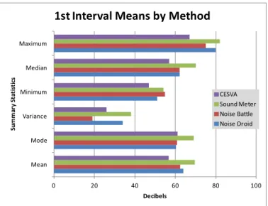
Figure 4: Graph of Summary Statistics First Interval Means by Method

Figure 4 shows summary statistics for the four methods of sound measurement. The Sound Meter measurements are consistently higher than the rest. The range for maximums is high, while minimums are fairly close together. The medians are similar with the exception of Sound Meter at 10 decibels higher. Although the means are not that dissimilar, the variances differ more greatly than any other statistic. The modes for each method are close to the means for the same method. Figure 5 shows that the variations in spatial locations between highs and lows in the four datasets are apparently random.

(32)

20

Figure 6: Maps of Kriging First Interval Measurements

(33)

21

4.1.1.2 Second Interval

45 50 55 60 65 70 75 80 85

De

cib

e

ls

2nd Interval Means by Method

Figure 7: Graph of Second Interval Means by Method

As is visible in Figure 7, the second interval is nearly identical to the first, with fewer Noise Droid extremes on the high end. Noise Droid and Noise Battle measurements lie in the same range, slightly above the CESVA measurements.

Noise Droid 62 30

Noise Battle 62 19

Sound Meter 68 38

CESVA 55 33

63.04(2.19E-30)

Table 7: ANOVA Second Interval Means by Method

(34)

22

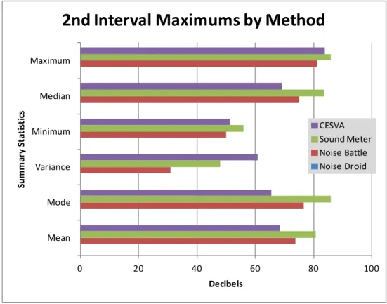
0 20 40 60 80 100

Mean Mode Variance Minimum Median Maximum

Decibels

S

u

m

a

ry

S

ta

ti

sti

cs

2nd Interval Means by Method

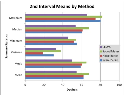
Figure 8: Graph of Summary Statistics Second Interval Means by Method

Figure 8 shows that Sound Meter has the highest statistics again, except the Noise Droid minimum is higher. Again, Noise Battle has the smallest variance and the variances are all very different. The modes, especially CESVA, are lower than the means. Noise Battle and Noise Droid share the same mean and nearly the same median. Figure 9 shows that the variations in spatial locations between highs and lows in the four datasets are apparently random.

(35)

23

Figure 10: Maps of Kriging Second Interval Measurements

(36)

24

4.1.1.3 Third Interval

45 50 55 60 65 70 75 80 85

De

cib

e

ls

3rd Interval Means by Method

Figure 11: Graph of Third Interval Means by Method

In Figure 11, it is apparent that the measurements are more consolidated along the same plane, congruent to that of the CESVA progression. This is the interval during which the Sound Meter measurements are closest to the rest, with fewer extremes and smaller differences. Noise Battle still drops below CESVA in a few of the same spots as the morning intervals.

Noise Droid 62 28

Noise Battle 61 16

Sound Meter 66 31

CESVA 56 30

46.08(6.71E-24)

Table 8: ANOVA Third Interval Means by Method

(37)

25

0 20 40 60 80 100

Decibels

S

u

m

a

ry

S

ta

ti

sti

cs

3rd Interval Means by Method

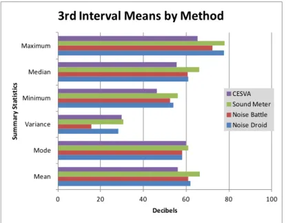
Figure 12: Graph of Summary Statistics Third Interval Means by Method

In Figure 12, it can be seen that Sound Meter is still the leader in high values, but not by as large a difference as in earlier intervals. Noise Droid recorded the same maximum as Sound Meter and Noise Droid and Noise Battle recorded the same mode. The variances for all but Noise Battle are close this time. CESVA has the lowest statistics except for variance and mode. Figure 13 shows that the variations in spatial locations between highs and lows in the four datasets are apparently random.

(38)

26

Figure 14: Maps of Kriging Third Interval Measurements

(39)

27

4.1.1.4 Fourth Interval

45 50 55 60 65 70 75 80 85

De

cib

e

ls

4th Interval Means by Method

Figure 15: Graph of Fourth Interval Means by Method

In Figure 15, it can be seen that the distribution is similar to the previous interval, but with more high decibel level extremes in the Sound Meter dataset. The three smart phone applications follow the same general progression as CESVA, only 10 to 20 decibels higher. It is important to keep in mind that a 10 decibel increase sounds twice as loud and a 20 decibel increase sounds four times as loud. Therefore, the sound scheme recorded by the three phone methods is significantly different than that recorded by the professional CESVA.

Noise Droid 62 21

Noise Battle 62 18

Sound Meter 67 25

CESVA 56 27

57.01(2.36E-28)

Table 9: ANOVA Fourth Interval Means by Method

(40)

28

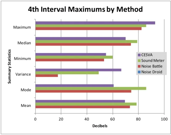
0 20 40 60 80 100

Decibels

S

u

m

a

ry

S

ta

ti

sti

cs

4th Interval Means by Method

CESVA

Sound Meter

Noise Battle

Noise Droid

Figure 16: Graph of Summary Statistics Fourth Interval Means by Method

In Figure 16 it can be seen that the variances are closer than any other interval so far, yet ANOVA revealed they are still statistically different. This time the Sound Meter maximum was surpassed by Noise Droid. CESVA values are lower than the rest, except for the variance. The means are higher than the modes. Figure 17 shows that the variations in spatial locations between highs and lows in the four datasets are apparently random.

(41)

29

Figure 18: Maps of Kriging Fourth Interval Measurements

(42)

30 4.1.2 Maximums

4.1.2.1 First Interval

For this section, there is no Noise Droid dataset since maximums were not recorded by that application. It remains in the legend to preserve the consistent color scheme.

50 55 60 65 70 75 80 85 90 95

De

cib

e

ls

1st Interval Maximums by Method

Figure 19: Graph of First Interval Maximums by Method

Figure 19 shows the maximums for each dataset during the first interval. Sound Meter records the highest values but the upper limit is only 86 decibels, so any sound louder than that will still be recorded at 86. Note that the CESVA values which correspond to these maximums range from 74 to 83. Noise Battle measurements are again concentrated in a band mostly above the CESVA values, with a few low extremes.

Noise Battle 72 23

Sound Meter 82 38

CESVA 70 54

61.67(1.96E-21)

Table 10: ANOVA First Interval Maximums by Method

(43)

31

0 20 40 60 80 100

Decibels

S

u

m

a

ry

S

ta

ti

sti

cs

1st Interval Maximums by Method

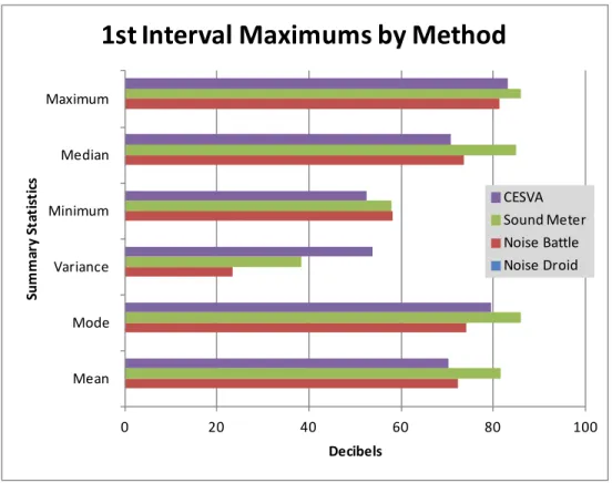
Figure 20: Graph of Summary Statistics First Interval Means by Method

(44)

32

4.1.2.2 Second Interval

50 55 60 65 70 75 80 85 90 95

De

cib

e

ls

2nd Interval Maximums by Method

Figure 21: Graph of Second Interval Maximums by Method

In Figure 21, it can be seen that more of the Noise Battle measurements are higher compared to CESVA than in the last interval. There are also three measurements lower than CESVA at the lower end. Also, around one-third of the Sound Meter measurements are at the upper limit of 86, and nearly one-half are above 80 decibels. For the first time so far, all the Sound Meter measurements are higher than the CESVA values. This is due to extremely high winds the day the measurements were taken and is discussed in detail in another section.

Noise Battle 74 31

Sound Meter 81 48

CESVA 68 61

56.14(5.79E-20)

Table 11: ANOVA Second Interval Maximums by Method

(45)

33

0 20 40 60 80 100

Decibels

S

u

m

a

ry

S

ta

ti

sti

cs

2nd Interval Maximums by Method

Figure 22: Graph of Summary Statistics Second Interval Maximums by Method

(46)

34

4.1.2.3 Third Interval

50 55 60 65 70 75 80 85 90 95

De

cib

e

ls

3rd Interval Maximums by Method

Figure 23: Graph of Third Interval Maximums by Method

Figure 23 tells almost the same story as the previous morning’s datasets, except for a few important differences. There are a few low extremes for both Noise Battle and Sound Meter. Also, this is the first time CESVA hits the 85 decibel level mark, but it only happens once in this interval.

Noise Battle 73 21

Sound Meter 79 53

CESVA 70 50

29.57(6.06E-12)

Table 12: ANOVA Third Interval Maximums by Method

(47)

35

0 20 40 60 80 100

Decibels

S

u

m

a

ry

S

ta

ti

sti

cs

3rd Interval Maximums by Method

Figure 24: Graph of Summary Statistics Third Interval Maximums by Method

(48)

36

4.1.2.4 Fourth Interval

50 55 60 65 70 75 80 85 90 95

De

cib

e

ls

4th Interval Maximums by Method

Figure 25: Graph of Fourth Interval Maximums by Method

Figure 26 shows that the fourth interval Sound Meter measurements have dropped quite a bit, and while there are still many above 80 decibels, there are more in the 70 to 80 range. For the second time, none of the Sound Meter values are below those of CESVA. Noise Battle stays in the usual range with only two extreme lows this interval. There is also an abnormality which may be attributed to human error. There is one CESVA measurement at 93 decibels, which is nine decibels (almost twice as loud) as its next highest measurement. It is most likely that some interference occurred with the microphone to cause this extremely high measurement. Unlike the smart phone applications, the CESVA’s upper limit is not 86decibels, but 137, so it is possible that this was the actual maximum recorded at the time.

Noise Battle 73 17

Sound Meter 79 49

CESVA 70 67

30.63(2.71E-12)

Table 13: ANOVA Fourth Interval Maximums by Method

(49)

37

0 20 40 60 80 100

Decibels

S

u

m

a

ry

S

ta

ti

sti

cs

4th Interval Maximums by Method

Figure 26: Graph of Summary Statistics Fourth Interval Maximums by Method

(50)

38

4.1.3 All measurements for all intervals together by method

4.1.3.1 Means

45 50 55 60 65 70 75 80 85 De cib e ls

Means

Figure 27: Graph of All Means by Method

Figure 27 shows all 264 measurements (66 for each of the four intervals) for each of the four methods. They are organized by CESVA least to greatest. The majority of smart phone measurements are above those of the professional sound meter. Most of the Noise Droid and Noise Battle measurements are 5 to 10 decibels higher (10 is twice as loud), with the high extremes as much as 20 to 25 decibels higher (20 is four times as loud). Most of the Sound Meter measurements are 10 to 15 decibels higher and the high extremes are up to 30 decibels louder. None of the Sound Meter means are lower than CESVA. In the upper range of CESVA measurements, there are several Noise Droid and Noise Battle measurements that are lower than the CESVA measurements, and most are within 10 decibels less (half as loud).

Noise Droid 62 28

Noise Battle 62 18

Sound Meter 68 34

CESVA 56 29

226.06(1.3E-112)

Table 14: ANOVA All Means by Method

(51)

39

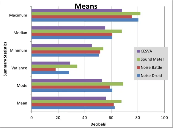
0 20 40 60 80 100

Decibels

S

u

m

a

ry

S

ta

ti

sti

cs

Means

Figure 28: Graph of Summary Statistics All Means by Interval

(52)

40

4.1.3.2 Maximums

50 55 60 65 70 75 80 85 90 95

De

cib

e

ls

Maximums

Figure 29: Graph of All Maximums by Method

Figure 29 shows all the maximum values from all four intervals combined into one dataset for each method except for Noise Droid, the software for which did not upload maximums. The datasets are matched to the progression of CESVA values from least to greatest. The Noise Battle measurements are all in roughly the same range, from 70 to 77 decibels. The majority of them are above the CESVA measurements, although several are below and a few are very far below. Unlike the means, a few of the Sound Meter maximums are below those for CESVA.

Noise Battle 73 23

Sound Meter 80 48

CESVA 70 58

168.98(9.07E-62)

Table 15: ANOVA All Maximums by Method

(53)

41

0 20 40 60 80 100

Decibels

S

u

m

a

ry

S

ta

ti

sti

cs

Maximums

Figure 30: Graph of Summary Statistics All Maximums by Method

(54)

42

4.2 Comparisons of smart phone applications to CESVA sound level meter

with t-Tests

In the previous section it was shown through the ANOVA testing that there is a statistically significant difference between the four test groups - sound measurements taken using the three smart phone applications and the professional sound level meter. In this section the author uses a variety of tools to compare only two datasets at a time in order to show exactly where these differences lie. Instead of looking at each interval separately, the full set of measurements for all four intervals are combined as in the final two ANOVA analyses. Each of the smart phone application datasets is compared to the CESVA dataset in a Student’s t-Test (also known as a one-way analysis of variance test), run in Microsoft Excel 2007, with the results reported followed by a brief commentary. First the t-Test: Two-Sample Assuming Equal Variances was run, and if the variances are not equal, the t-Test: Two-Sample Assuming Unequal Variances was run. The results are reported as means, variances , the t-Statistic used to run the test, and the resulting p-value in parentheses. When the p-value is less than the 0.05 (5%) Alpha (for a 95% confidence interval), the null hypothesis that the means are the same must be rejected and the conclusion is that the means are statistically significantly different. An assumption of t-Tests is that the datasets being compared are normally distributed, but because this data is in a logarithmic scale, it is already somewhat so.

For this analysis, the difference between each paired measurement has been calculated and plotted with the smart phone and CESVA datasets. In each instance, the difference is the smart phone measurement minus the CESVA measurement. The scatter plots are organized by the difference value from least to greatest, with the paired measurements above them on the same scale.

To validate the smart phone measurements against those taken by the CESVA, the sets are plotted against each other in a scatter plot. CESVA is the “measured decibel level” on the x-axis and the smart phone application is the “predicted decibel level” on the y-axis. The scale is the same for both axes, from 45 to 85 decibels for the means comparisons and from 50 to 90 decibels for the maximums comparisons. The blue line is the 45° degree line which, if the points fall along it, represents a one to one relationship and would validate the accuracy of the “prediction.” The black line is the actual linear trend line for the smart phone data. Comparing the two both illustrates and quantifies the tendency of inaccuracy recorded by the smart phones compared with the professionally calibrated sound level meter.

For further illustration, a histogram of each dataset is presented, with frequency on the y-axis and decibels on the x-axis. The scale of zero to 160 for frequency is used consistently for easy, unbiased visual comparison. Note that the way the histogram organizes the values may be misleading. Each value is rounded up and placed in a bin, and the numbers labeling the bins on the x-axis denote the highest value allowed in that bin. In other words, numbers from -10 to -5 fall into the -5 bin, and numbers from -4.9 to zero fall into the zero bin. For example, a value of -5.5 falls into the -5 bin, a -4.5 value falls into the zero bin and a 1.5 value falls into the 5 bin. This is important because not all the values in the zero bin are actually zero. Comments are given with each set of charts, and discussion follows at the end.

(55)

43

the differences between the values in these datasets may seem small, these measurement devices are depicting two very different representations of the real world.

Here is the organization of the analysis which follows:

Means compared to CESVA Noise Droid

Noise Battle Sound Meter

Maximums compared to CESVA Noise Battle

(56)

44 4.2.1 Means compared to CESVA

4.2.1.1 Noise Droid Means

Figure 31: Graph of Noise Droid Means compared to CESVA Means

(57)

45

Mean Variance t-Statistic

Noise Droid 62 28

CESVA 56 29 13.89(2.29E-37)

Table 16: t-Test of Noise Droid and CESVA Means

Table 16 shows the results of the t-Test for this subgroup. The value of the statistical test used to compare the means is 13.89. The p-value is less than 5%, so the Noise Droid and CESVA means are statistically significantly different.

Figure 32: Noise Droid Means Cross Validation Graph

(58)

46 0 20 40 60 80 100 120 140 160

45 50 55 60 65 70 75 80 85

Fr e q u e n cy Decibels

Noise Droid Means

0 20 40 60 80 100 120 140 160

45 50 55 60 65 70 75 80 85

CESVA Means

0 20 40 60 80 100 120 140 160

-10 -5 0 5 10 15 20 25 30

Fr e q u e n cy

Difference in Decibels

Means Difference: Noise Droid - CESVA

Figure 33: Histograms of Noise Droid Means, CESVA Means and their Means Difference

(59)

47

(60)

48

4.2.1.2 Noise Battle Means

Figure 34: Graph of Noise Battle Means compared to CESVA Means

(61)

49

Noise Battle 62 18

CESVA 56 29 14.06(4.62E-38)

Table 17: t-Test of Noise Battle and CESVA Means

Table 17 shows the results of the t-Test for this subgroup. The value of the statistical test used to compare the means is 14.06. The p-value is less than 5%, so the Noise Battle and CESVA means are statistically significantly different.

Figure 35: Noise Battle Means Cross Validation Graph

(62)

50 0 20 40 60 80 100 120 140 160

45 50 55 60 65 70 75 80 85

Noise Battle Means

0 20 40 60 80 100 120 140 160

45 50 55 60 65 70 75 80 85

CESVA Means

0 20 40 60 80 100 120 140 160

-10 -5 0 5 10 15 20 25 30

Fr e q u e n cy

Means Difference: Noise Battle - CESVA

Figure 36: Histograms of Noise Battle Means, CESVA Means and their Means Difference

(63)

51

(64)

52

4.2.1.3 Sound Meter Means

Figure 37: Graph of Sound Meter Means compared to CESVA Means

(65)

53

Sound Meter 68 34

CESVA 56 29 24.18(3.05E-87)

Table 18: t-Test of Sound Meter and CESVA Means

Table 18 shows the results of the t-Test for this subgroup. The value of the statistical test used to compare the means is 24.18. The p-value is far less than 5%, so the Sound Meter and CESVA means are statistically significantly different.

Figure 38: Sound Meter Means Cross Validation Graph

(66)

54 0 20 40 60 80 100 120 140 160

45 50 55 60 65 70 75 80 85

Sound Meter Means

0 20 40 60 80 100 120 140 160

45 50 55 60 65 70 75 80 85

CESVA Means

0 20 40 60 80 100 120 140 160

-10 -5 0 5 10 15 20 25 30

Fr e q u e n cy

Means Difference: Sound Meter - CESVA

Figure 39: Histograms of Sound Meter Means, CESVA Means and their Means Difference

(67)

55

(68)

56 4.2.2 Maximums compared to CESVA

4.2.2.1 Noise Battle Maximums

Figure 40: Graph of Noise Battle Maximums compared to CESVA Maximums

(69)

57

Noise Battle 73 23

CESVA 70 58 6.27(8.41E-10)

Table 19: t-Test of Noise Battle and CESVA Maximums

Table 19 shows the results of the t-Test for this subgroup. The value of the statistical test used to compare the means is 6.27. The p-value is less than 5%, so the Noise Battle and CESVA maximums are statistically significantly different.

Figure 41: Noise Battle Maximums Cross Validation Graph

(70)

58 0 20 40 60 80 100 120 140 160

50 55 60 65 70 75 80 85 90 95

Noise Battle Maximums

0 20 40 60 80 100 120 140 160

50 55 60 65 70 75 80 85 90 95

CESVA Maximums

0 20 40 60 80 100 120 140 160

-25 -20 -15 -10 -5 0 5 10 15 20 25 30

Fr e q u e n cy

Maximums Difference: Noise Battle - CESVA

Figure 42: Histograms of Noise Battle Maximums, CESVA Maximums and their Maximums Difference

(71)

59

(72)

60

4.2.2.2 Sound Meter Maximums

Figure 43: Graph of Sound Meter Maximums compared to CESVA Maximums

(73)

61

Sound Meter 80 48

CESVA 70 58 16.29(1.49E-48)

Table 20: t-Test of Sound Meter and CESVA Maximums

Table 20 shows the results of the t-Test for this subgroup. The value of the statistical test used to compare the means is 16.29. The p-value is less than 5%, so the Sound Meter and CESVA maximums are statistically significantly different.

Figure 44: Sound Meter Maximums Cross Validation Graph